Article

A Machine Learning Framework towards Bank Telemarketing Prediction

by
Stéphane Cédric Koumétio Tékouabou
1,2,*,
Ştefan Cristian Gherghina
3,*,
Hamza Toulni
4,5,
Pedro Neves Mata
6,7,
Mário Nuno Mata
6 and
José Moleiro Martins
6,8
1
Center of Urban Systems (CUS), Mohammed VI Polytechnic University (UM6P), Hay Moulay Rachid, Ben Guerir 43150, Morocco
2
Laboratory LAROSERI, Department of Computer Science, Faculty of Sciences, Chouaib Doukkali University, El Jadida 24000, Morocco
3
Department of Finance, Bucharest University of Economic Studies, 6 Piata Romana, 010374 Bucharest, Romania
4
EIGSI, 282 Route of the Oasis, Mâarif, Casablanca 20140, Morocco
5
LIMSAD Laboratory, Faculty of Sciences Ain Chock, Hassan II University of Casablanca, Casablanca 20100, Morocco
6
ISCAL-Instituto Superior de Contabilidade e Administraçäo de Lisboa, Instituto Politécnico de Lisboa, Avenida Miguel Bombarda 20, 1069-035 Lisboa, Portugal
7
Microsoft (CSS-Microsoft Customer Service and Support Department), Rua Do Fogo de Santelmo, Lote 2.07.02, 1990-110 Lisboa, Portugal
8
Business Research Unit (BRU-IUL), Instituto Universitário de Lisboa (ISCTE-IUL), 1649-026 Lisboa, Portugal
*
Authors to whom correspondence should be addressed.
J. Risk Financial Manag. 2022, 15(6), 269; https://doi.org/10.3390/jrfm15060269
Submission received: 7 May 2022 / Revised: 7 June 2022 / Accepted: 13 June 2022 / Published: 16 June 2022
(This article belongs to the Special Issue Innovative Financial Econometrics and Machine Learning)

Abstract

:
The use of machine learning (ML) methods has been widely discussed for over a decade. The search for the optimal model is still a challenge that researchers seek to address. Despite advances in current work that surpass the limitations of previous ones, research still faces new challenges in every field. For the automatic targeting of customers in a banking telemarketing campaign, the use of ML-based approaches in previous work has not been able to show transparency in the processing of heterogeneous data, achieve optimal performance or use minimal resources. In this paper, we introduce a class membership-based (CMB) classifier which is a transparent approach well adapted to heterogeneous data that exploits nominal variables in the decision function. These dummy variables are often either suppressed or coded in an arbitrary way in most works without really evaluating their impact on the final performance of the models. In many cases, their coding either favours or disfavours the learning model performance without necessarily reflecting reality, which leads to over-fitting or decreased performance. In this work, we applied the CMB approach to data from a bank telemarketing campaign to build an optimal model for predicting potential customers before launching a campaign. The results obtained suggest that the CMB approach can predict the success of future prospecting more accurately than previous work. Furthermore, in addition to its better performance in terms of accuracy (97.3%), the model also gives a very close score for the AUC (95.9%), showing its stability, which would be very unfavourable to over-fitting.

1. Introduction

A marketing campaign is a set of commercial operations all pursuing the same objective, which may concern the improvement of brand awareness and/or sales objectives (Leppäniemi and Karjaluoto 2008). These operations can take different forms and be spread out over time or be concomitant. If in the past the majority of commercial operations were based on mass marketing, nowadays direct or even targeted marketing is more and more desired (Koumétio et al. 2018; Tekouabou et al. 2019). Companies use direct marketing strategies when they target customer segments by contacting them to achieve a specific sales campaign (Moro et al. 2014). To facilitate the operational management of campaigns, they centralise remote interactions in a contact centre (Feng et al. 2022). The latter contains all the strategic data on customers or potential customers for help, assistance, loyalty and the realisation of new business (Ballings and Van den Poel 2015). Such centres allow communication with customers through different channels: postal mail, email, SMS or, better yet, telephone calls (on landline or mobile). Recently, the telephone has become one of the most widely used means of managing customer relations (Moro et al. 2011, 2014), especially with the possibility of transmitting from the internet, using voice on internet protocol (VoIP) techniques, which have drastically reduced the cost of calls while ensuring greater security (Butcher et al. 2007). This marketing technique implemented through a contact centre is called telemarketing because of the characteristic of remoteness (Kotler and Keller 2016; Moro et al. 2014). Telemarketing has proven to be more practical and efficient with the remote working conditions imposed to deal with the recent pandemic related to COVID-19 (Sihombing and Nasib 2020). Telemarketing is becoming more and more reliable both for customers and for companies wanting to opt for this marketing strategy (Butcher et al. 2007; Feng et al. 2022). In addition to these different advantages, the technique allows for a rethinking of marketing by focusing on maximising the value of the customer throughout his or her life, thanks to the evaluation of the available information and the customisation of the targeting parameters (Bhattacharyya et al. 2011; Cioca et al. 2013). Thanks to technological evolution, notably, the processing capacities of machines and the volumes of storage, this information collected on customers is increasingly rich and varied (Koumétio and Toulni 2021). On the other hand, the emergence of machine learning algorithms and data mining tools for which these data constitute the raw material (Al-Garadi et al. 2020). These algorithms allow for a more efficient evaluation of these data to predict the results of the marketing campaigns, or even the complete automation of the operation (Moro et al. 2014). The forecasts allow, in the majority of cases, an operational adjustment to build longer and closer relationships, according to the demand of the companies (Rust et al. 2010).
The data collected and thus currently enriched for more realistic predictive targeting suffer from several problems, such as volume, complexity and especially heterogeneity, which negatively affect the performance of the algorithms (Al-Garadi et al. 2020; Koumétio and Toulni 2021). Thus, the classification algorithms currently used are limited not only by the data size, which makes them slower and weakens their performance, but by the feature scale difference, which makes them unstable, the data heterogeneity, and above all the non-numerical data, which require a more sophisticated or even complex preprocessing (Al-Garadi et al. 2020; Bhattacharyya et al. 2011; Cioca et al. 2013). This should be set up, regulated, adjusted and transparently processed during the machine learning model design, especially for heterogeneous data, such as those of the UCI Portuguese bank telemarketing dataset (Tekouabou et al. 2019). However, several works do not mention the preprocessing steps applied in their experiments (Koumétio and Toulni 2021; Moro et al. 2014; Tekouabou et al. 2019; Vafeiadis et al. 2015; Vajiramedhin and Suebsing 2014). Moreover, previous works have examined conventional classification techniques as well as classical data mining methods (SVM, DT, KNN, NB, ANN, …) or emerging ensemble methods (RF, Bagging, GB, …). However, these methods present a problem of mismatch with multiple features and are prone to data leakage when re-training the machine learning model (Turkmen 2021). Even though some studies involving these methods have achieved high performance, the experimental protocols are often very unreliable to really assess the feasibility of the performance achieved in these works (Koumétio and Toulni 2021; Moro et al. 2014; Tekouabou et al. 2019; Vafeiadis et al. 2015; 
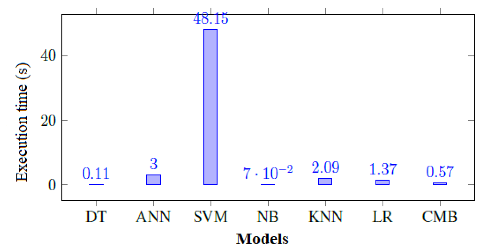
Vajiramedhin and Suebsing 2014). Among the works investigated on this problem, many have evoked the problem of execution time without really calculating it; this is the case of (Farooqi and Iqbal 2019). However, the execution time is very important to evaluate the algorithmic complexity of a machine learning approach (Cherif 2018; Koumétio et al. 2018). On the other hand, the metrics often used to evaluate their performances are either unsuitable or insufficient to evaluate this type of problem (Koumétio and Toulni 2021; Tekouabou et al. 2019) (classification of imbalanced data Marinakos and Daskalaki 2017). Of course, this is not to mention the sometimes depreciated and unreliable experimentation tools (SPSS, Rapidminer, WEKA), which allow for relatively dubious models.
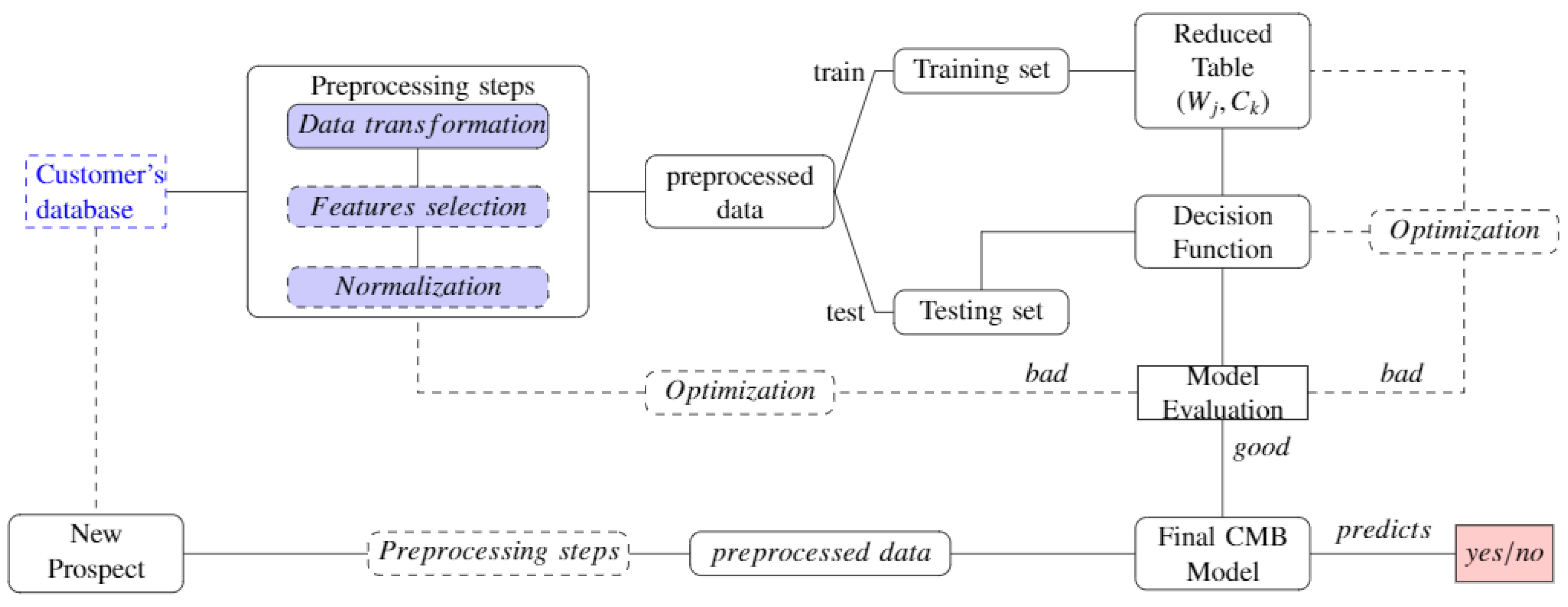
Hence, we propose in this paper a new approach based on membership classes (CMB). The CMB approach is devoted to achieving the best performance of realistic prediction by transforming the heterogeneous data used. Therefore, it will overcome the main challenge of current ML algorithms by well processing each type of these heterogeneous data. Optimising the transformation of this mosaic datasets’ features for better prediction performance is the first goal we seek to achieve during preprocessing. What makes our method different from other existing algorithms is that the preprocessing of nominal-type features that are difficult to process in the existing approaches so far simply involves imputing the missing values. The nominal features are directly used in the class membership-based (CMB) classification phase process. This and the elimination of non-significant attributes allow the processing time, which constitutes the second challenge of our approach. Generally, transformed data present a problem with different variable scales. Standardisation is an additional step in dealing with this problem, but it has an adverse or favourable effect on the performance of certain algorithms that are said to be unstable to variable scales, knowing that a very large-scale difference is more favourable for over-fitting. We have, therefore, created the proposed classification algorithm, which, from the reduced table of the training database, independently classifies each attribute before predicting the class of the individual. This is the third contribution of our paper.
Basically, the contribution of this paper is summarised in the following points:
  • The introduction of a novel approach that processes heterogeneous data by transforming separately each type of feature (numerical, Boolean, scaled and nominal), then a hybrid technique to replace missing values and implicitly select the most significant features. This helps to optimise the classification in terms of processing time and accuracy. Apart from the replacement of missing values, we do not transform nominal attributes in this step because they are directly treated in the classification; this allows reducing the processing time.
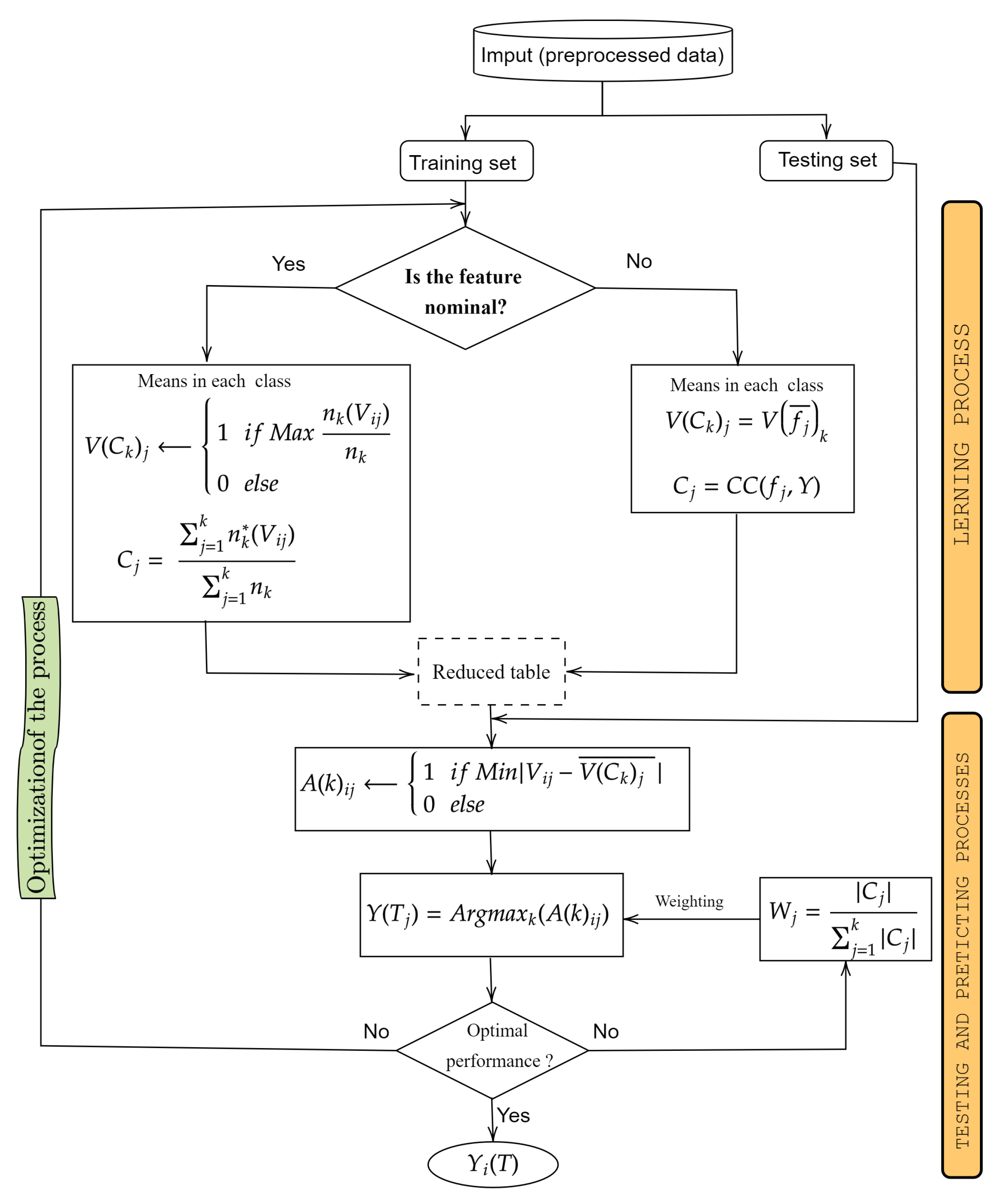
  • The construction of the reduced table of training data. For each class, this table contains the averages of transformed features and the favourable attributes for nominal features.
  • A simplification of the overall approach for the special case of binary classification. It incorporates a weighting scheme that improves the performance.
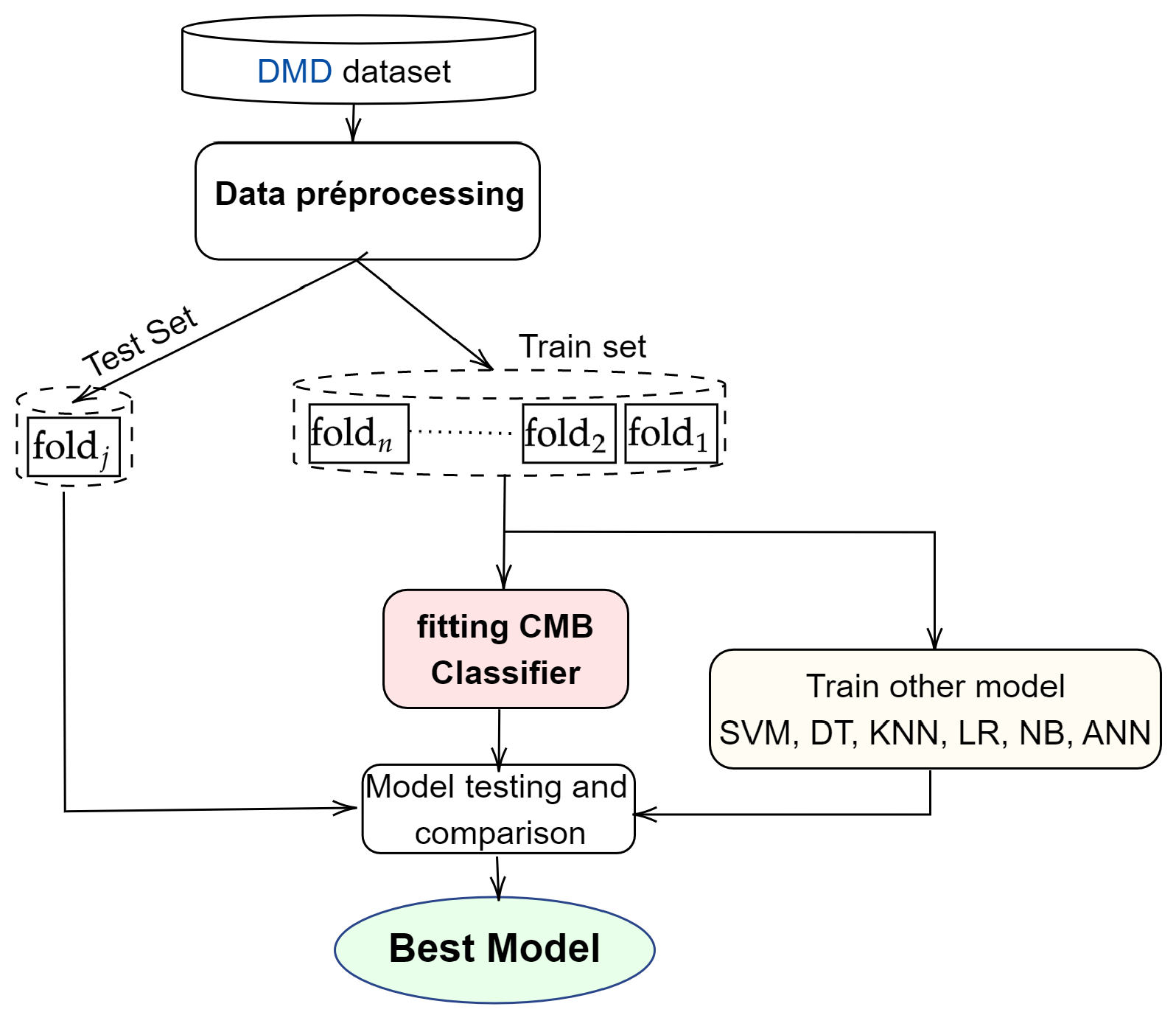
  • Proposing and following a clear and transparent design and implementation process to efficiently solve a real and concrete machine learning problem.
  • The successful implementation and use of the model designed to optimise the predictive performance of potential leads before a telemarketing bank campaign.
Following this work, Section 2 and Section 3 investigate the related works and depict the proposed method, which constructs a class membership-based approach, respectively. Then, Section 4 analyses the experimental results performance of our model, while Section 5 discusses these results. Finally, Section 6 concludes our study.

2. Prior Literature Review

The banking telemarketing database was first used by (Moro et al. 2011) in 2011, who processed this data with the RapidMiner tool. Its second version collected data from 2008 to 2012, and allowed the publication of the article (Moro et al. 2014) and the data shared for research. Since then, this dataset has heavily affected the field of machine learning, occupying the seventh most popular data position on the UCI Machine Learning repository1 It is a reference for the training and tuning of new models and even a pedagogical or research tool in data science. Thus, several articles using a multitude of approaches have been published on the subject of predicting the success of a telemarketing bank campaign (Feng et al. 2022; Govindarajan 2016; Koumétio and Toulni 2021; Tekouabou et al. 2019). The best papers published in this issue were selected by searching for “bank telemarketing” AND “machine learning” request in different databases (Google Scholars, WoS, and Scopus) and the list was completed by citation matching. The summary of these papers is presented in Table 1. From the point of view of the type of learning, it is supervised learning and a very unbalanced classification problem (Miguéis et al. 2017; Thakar et al. 2018). The unbalanced classification often imposes the use of certain metrics, such as AUC, f 1 -score, or G m e a n to determine the best model, especially since the target class is often a minority. This is one of the limitations of the majority of papers published on this problem. Some authors have used data-balancing techniques (SMOTE Chawla et al. 2002; RAMO Chen et al. 2010) before training the models (Krawczyk 2016; Marinakos and Daskalaki 2017). These approaches are limited by the fact that they create random instances that do not always reflect reality and, in addition, increase the processing time of the algorithms and thus the complexity of the models. On the other hand, since the data are heterogeneous, i.e., contain variables of several types, very few authors have shown transparent approaches allowing to understand the data pre-processing steps before training the models (Koumétio et al. 2018; Koumétio and Toulni 2021; Tekouabou et al. 2019).
The methods used range from classical learning methods to deep learning methods and ensemble methods. While early works focused on simple learning methods, such as DT, SVM, NB, ANN, KNN or LR (Elsalamony and Elsayad 2013; Elsalamony 2014; Karim and Rahman 2013; Moro et al. 2011, 2014, 2015; Vajiramedhin and Suebsing 2014), more complex approaches or combinations of several simple methods have since been used (Amini et al. 2015; Govindarajan 2016). These simple models have achieved the best performance in several works, although the experimental protocol often raises questions about the results. S. Moro et al. (Moro et al. 2011, 2014, 2015) for example, used simple learning methods (DT, SVM, NB, ANN, LR, and KNN) but using the ALIFT chart to show the proportion of favourable prospects according to the model. Generally, the works on this topic pose a problem of performance reliability linked to the simulation tool (Rapid Miner). The DT model was found to perform better according to the results of (Farooqi and Iqbal 2019; Karim and Rahman 2013; Koumétio et al. 2018; Tekouabou et al. 2019; Vajiramedhin and Suebsing 2014) and seems to be globally one of the best models for this problem by compromising performance and complexity. However, DT is still very much in favour of the over-fitting that would affect this performance in reality. Hence, (Amini et al. 2015; Elsalamony and Elsayad 2013; Govindarajan 2016) have proposed ensemble methods to try to overcome these limitations. Other authors, on the other hand, have proposed their models based on the modification or improvement of classical models. This is the case of (Tekouabou et al. 2019), who proposed an improvement of the KNN model, while (Yan et al. 2020) proposed a model called the S _ K o h o n e n network and (Ghatasheh et al. 2020) the CostSensitive-MLP. (Birant 2020) introduced a method called the class-based weighted decision jungle, which is very sensitive to class imbalance, while Moro et al. (2018) and Lahmiri (2017) used a divide-and-conquer strategy and two-step based system, respectively. Manipulation of this class imbalance was included in the approaches adopted by (Krawczyk 2016; Marinakos and Daskalaki 2017; Miguéis et al. 2017; Thakar et al. 2018) to overcome the problem. (Elsalamony 2014; 
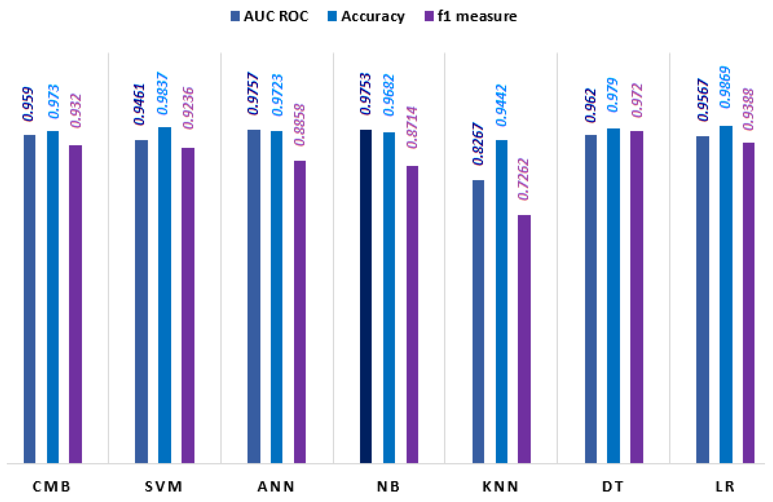
Ładyżyński et al. 2019) used models based on artificial or deep neural networks, which are sometimes slow and unsuitable for this type of data. The ANN model provided the best scores in the work of (Mustapha and Alsufyani 2019; Selma 2020) with 98.93% and 95.00% for accuracy and the f 1 score, respectively.
More recently, Feng et al. (Feng et al. 2022) used Python frameworks to implement ensemble methods with dynamic selection to predict sales in this campaign. Khalilpour Darzi et al. (2021) introduced a correlation-augmented naive Bayes (CAN) algorithm as a novel Bayesian method supposed to be well adjusted for direct marketing prediction. However, the performance of his model is still quite limited compared to previous works and his model is a bit more complex. Moreover, the transparent problem of preprocessing heterogeneous data and interpretability of the constructed model still persists. This is the main motivation for the approach we propose in the next section.

3. The Proposed Approach

This section is devoted to presenting our proposed approach which consists of two mean steps (see Figure 1): preprocessing and classification. The preprocessing transforms different types of features into a specific format, thus reducing the processing time and improving the classification performance while remaining very stable against variable scales by dealing with each attribute separately. To clearly illustrate these different steps, we begin by presenting the dataset used in Section 3.1.

3.1. Dataset

The direct marketing dataset (DMD) is actually a well-used dataset for predictive modelling in direct marketing. The goal is to rank the most likely customers to respond favourably to a marketing campaign. We used a direct marketing dataset that contains 45,000 customers from a Portuguese bank who were contacted by telephone between 2008 and 2012 and who received an offer to open a long-term deposit account with rates of attractive interest. Classes are unbalanced with less than 12% ranked “yes” and the rest classified as “no” (Moro et al. 2014). The dataset contains characteristics such as age, employment, marital status, educational level, average annual balance, and current loan status, as well as the class label, indicates whether the client accepted or not. From the presented dataset, let us consider an example of instances of the following Table 2 which contain some common features available in major customer datasets.

3.2. Data Preprocessing

The preprocessing step turns out to be very important for the prediction process because the performance closely depends. With the advent of big data, data are collected from several sources and are of different types: we treat heterogeneous data. Here, we propose a specific preprocessing in several phases: data transformation, replacing missing values, feature selection and finally standardisation again, later.

3.2.1. Data Transformation

The first step of our proposed technique consists of defining the type of the feature as the technique differs for either type. Table 1 illustrates four major types of features: numeric, Boolean, scaled and nominal (Tekouabou et al. 2021).
For numerical features ( f 1 ): We calculate directly the statistical parameters (min, max, mean, variance, and standard deviation) of each numerical feature.
For scaled Features ( f 4 ): We substitute items by their ordinal number. After that substitution, we calculate the statistical parameters.
For boolean features such as f 3 : For this type of feature, we have only two possibilities yes or no (1/0); success or failure (1/0); and telephone/cellular (1/0).
For nominal features (example of f 2 ): These features are considered independent features and are directly associated to the classification step for our approach. This reduces the processing time of all nominal features by almost half while improving performance. Such features are processed in the classification step.

3.2.2. Replacement of Missing Values

The problem of missing values is often very common in heterogeneous datasets, especially those collected from CRM, and is a challenge for optimal data modelling. One of the advantages of our approach is that it proposes a function allowing a fast and optimal imputation of the missing values according to the type of features to which they belong (Lakshminarayan et al. 1999). Such a function consists of replacing all the missing values V i j of the feature V j by the average if they are scaled or numerical variables or the mode if they are Boolean or nominal variables inside the class k:
( V i j ) k m i s s M o d e ( V j ) k if boolean or nominal M e a n ( V j ) k if numerical or scaled
For example, if we consider Table 3 below: V j = “ f 4 ” is a scaled variable; I 4 takes the value U n k n o w n for f 4 and k = “ y e s ”, M e a n ( V j ) y e s = ( 2 + 0 ) 2 = 1 ; the missed value is replaced by 1.

3.2.3. Features Selection

The analysis of correlations ( C ( f j , Y ) ) between feature ( f j ) and class Y allows not only to identify those correlated strongly to the label and therefore to contribute enough to the classification (Tripathi et al. 2018), but also reduces the feature space by setting a threshold. Weakly correlated variables that do not contribute to the decision and consume processing time are then ignored. They are neutral for classification decisions.
C j = C ( f j , Y ) = i = 1 n ( f i j f j ¯ ) . ( y i y ¯ ) i = 1 n ( f i j f j ¯ ) . i = 1 n ( y i y ¯ )
In our case, we set a threshold of 1%, which allows us to eliminate some variables (having C j < 0.01 ) and use only other ones which are significant for classification (Yu and Liu 2003). This only affects attributes initially numerical or Boolean types that were not transformed during the transformation phase.
After all preprocessing steps, the preprocessed table becomes as follows:
Table 3. Preprocessed data.
Inst. f 1 f 2 f 3 f 4 Label
I 1 59married010
I 2 39single121
I 3 59married000
I 4 41divorced011
I 5 44married001

3.2.4. Normalisation

The normalisation is used to eliminate the impact of the order of magnitude and is very important to optimise the machine learning model performance. It reduces each V i j to the interval [0,1] by the formula:
V i j V i j m i n j ( V i j ) m a x j ( V i j ) m i n j ( V i j )
The result of the normalisation of the previous Table 3 values is contained in the following Table 4.

3.3. Classification Process

The classification principle of the CMB approach is that for each feature, it compares the value of this feature for a new instance with the averages of this feature’s value in different classes. Then, based on this feature, it tentatively assigns the instance to the class for which the value of this feature is the closest to the corresponding average. Then, it adds weights of all the classes to which the object is tentatively based on different features, and for whatever class the weighted sum is largest, this is the class to which we classify the given object.
Thus, the proposed classification algorithm (Figure 2) contains two phases. The first is to build the reduced table of training data centred on each class, and the second is the decision phase.

3.3.1. Training: Reduced Table Construction

The training step consists of building the reduced table by calculating the centre C k of each class, which contains the average V ( f j ) k ¯ of the previously transformed numeric, scaled and Boolean features.
The particularity of this approach is how it deals with nominal independent features ( f 2 in Table 2). Each value of the nominal features V j for the example i can belong to class C k if its maximum class frequency is reached for this class in the training set; this frequency is given by the formula
V ( C k ) i j 1 if Max n k ( V i j ) N k 0 else
where
  • n k ( V i j ) is the number of V i j variables j in the class C k ;
  • N k is the total number of classes k.
The value 1 means that this attribute is more favourable to the class k and will be placed in C k for this variable in the reduced table and so on for all attributes of nominal variables. So, the nominal attribute takes the value 1 in this class k and 0 in other classes.
Belonging coefficient of nominal features:
As the correlation coefficient (Equation (2)) was used to weight the numerical variables in the reduced table, we introduce membership coefficients for the nominal features that are calculated from the belonging coefficients of each unique attribute to class k. It consists of the ratio between the sum of the maximum numbers of each unique attribute in class k and the number of instances (Equation (5)). For this formulation, let n k * ( V i j ) denote all the respective n k ( V i j ) values corresponding to the maximum, and we can deduce the belonging coefficient of the feature f j to the class as follows:
C j = j = 1 k n k * ( V i j ) j = 1 k N k
Let us consider Table 3:
  • The total number of yes is N y e s = 3;
  • The total number of no is N n o = 2;
  • The number of “ m a r r i e d ” in the class “ n o ” is: n k ( m a r r i e d ) = 2;
  • The number of “ m a r r i e d ” in the class “ y e s ” is: n k ( m a r r i e d ) = 1.
n n o ( m a r r i e d ) N n o = 2 2 = 1 ; n y e s ( m a r r i e d ) N y e s = 1 3 = 0.33
1 > 0.33 so, the belonging to the class “ n o ” of all marital attributes “ m a r r i e d ” is replaced by 1 and their belonging to the class “ y e s ” is 0 during the prediction. They are placed in C n o (centre of the class n o in reduced table) of the reduced table for the feature f 2 .
We can therefore deduce the belonging coefficient of the feature f 2 as follows.
Table 5 below represents the reduced table of our example. n k * ( m a r r i e d ) = 2 , n k * ( d i v o r c e d ) = 1 , n k * ( s i n g l e ) = 1 , C 2 = 2 + 1 + 1 2 + 3 = 4 5 .
As we stated in Section 3.2.1, the advantage of our approach is using the nominal variables directly in the decision function without transforming them. We compute the belonging coefficient to each class for each characteristic of this type of nominal variable. Then we classify the characteristics in one class or another based on the higher value obtained. After this operation on three characteristics, one of them (married) was more favourable to the class “no” while the other two (single; divorced) were more favourable to the class “yes”.

3.3.2. Testing: Decision Function

The decision phase is performed by majority voting in two steps. Given a new instance T i , we start by calculating the membership A ( k ) i j of each attribute V i j of T i to the class k centred in C k . This eliminates the impact of feature scales. The A ( k ) i j are calculated by the following function except for nominal variables already treated by the previous equation:
A ( k ) i j 1 if Min | V i j V ( C k ) j ¯ | 0 else
T i is thus implicitly transformed into k instances A ( k ) , making it possible to predict its class Y ( T i ) p r e d , which is the one with the maximum of the sum of the overall A ( k ) i j of its j attributes as shown by the following function:
Y ( T i ) = A r g m a x k ( A ( k ) ) = A r g m a x k j = 1 n ( W j A ( k ) i j )
where W j is the feature weight calculated as follows:
W j = | C j | j = 1 n | C j |
This weighting is the most interesting since it allows us to standardise the coefficients so that the class memberships are bounded between 0 and 1. We can therefore set a decision threshold ( δ ) according to the number of classes k and the measure of the performance used.
In the case of binary classification ( k = 2 ), the threshold is
δ = 1 k + / ϵ = 0.5 + / ϵ
where ϵ is an adjustment factor of the optimal threshold δ . We have
Y ( T i ) 1 if A ( y e s ) > δ 0 else
For example, let us consider the example in Table 2 as our training set. We want to predict the class Y ( T 1 ) of a new instance T 1 : {38; Single; yes; irregular}.
The transformation of T 1 following the preprocessing steps gives us T 1 : {38; Single; 1; 0}.
Considering the corresponding reduced table (Table 5), we can deduce the class membership of each feature as follows:
  • For the feature f 1 : | V 11 V ( C n o ) 1 ¯ | = | 38 59 | = 21 and
    | V 11 V ( C y e s ) 1 ¯ | = | 38 41.33 | = 3.33
    3.33 < 21 and so, A ( n o ) 11 = 0
    A ( y e s ) 11 = 1 and its relative weight is W 1 = 0.98 2.52 = 0.38
  • For the feature f 2 which is nominal, “ S i n g l e ” is more favourable to C y e s
    so, A ( n o ) 12 = 0 and A ( y e s ) 12 = 1
    and its relative weight is W 2 = 0.8 2.52 = 0.32
  • For the feature f 3 : | V 13 V ( C n o ) 3 ¯ | = | 1 0 | = 1 and
    | V 13 V ( C y e s ) 3 ¯ | = | 1 0.33 | = 0.66 .
    0.66 < 1 so, A ( n o ) 13 = 0 and A ( y e s ) 13 = 1
    and its relative weight is W 3 = 0.41 2.52 = 0.16
  • For the feature f 4 : | V 14 V ( C n o ) 4 ¯ | = | 0 0.5 | = 0.5 and
    | V 14 V ( C y e s ) 4 ¯ | = | 0 1 | = 1.
    0.5 < 1 so, A ( n o ) 13 = 1 and A ( y e s ) 13 = 0
    and its relative weight is W 4 = 0.33 2.52 = 0.13 .
We can therefore predict the class by calculating
  • A ( y e s ) = 1 0.38 + 1 0.32 + 0 0.16 + 1 0.13 = 0.83
  • A ( n o ) = 0 0.38 + 0 0.32 + 1 0.16 + 0 0.13 = 0.16
Y ( T 1 ) = A r g m a x ( A ( y e s ) , A ( n o ) ) = A ( y e s ) = 1 because 0.83 > 0.16 and that’s how T 1 will be predicted for the class “ y e s ”.
Referring to the formula in Equation (9), since it is a binary classification, we can simply deduce the class of T 1 as follows: A ( y e s ) = 1 0.38 + 1 0.32 + 0 0.16 + 1 0.13 = 0.83 and δ = 0.5   A ( y e s ) = 0.83 > 0.5 . Therefore, T 1 is predicted in the class “ y e s ”.
This makes the approach simpler, faster and easy to optimise.

4. Results analysis and Discussion

4.1. Experimental Protocol

After acquiring the data as described in Section 3.1, we trained, tested and evaluated the proposed model as well as the other models by following the steps described in Figure 3. The first protocol step consists of transforming the data and missing values, with the unscaled nominal variables included in the decision function described in Section 3.3.2. The entire dataset was then divided five-fold, four of which were used for training and one for testing. All experiments were performed on a Windows operating system. All codes were written in the Python 3.7 programming language with the associated free ML library, the Scikit-learn library (Pedregosa et al. 2011). The computer used is an “Asus” computer with the following configuration: 8 GB of RAM, an Intel Core i7 processor and an NVIDIA Geforce 930 M graphics card.
After training, calibrating and evaluating the proposed model, we also trained, tested and compared other models that have shown good performance for this type of problem in the literature. Thus, the performance metrics used are described in the next section.

4.2. Performance Measure

The predictive accuracy rate Equation (11) is the most commonly used measure but it is not an effective tool for evaluating models on unbalanced datasets because it does not indicate how the model correctly classified the minority class instances that are often the targets. With regard to our databases which are unbalanced (Marinakos and Daskalaki 2017), we evaluate our approach in terms of other performance measures:
A c c u r a c y = a + b a + b + c + d
f 1 -score (FM) from Equation (12), is a classification metric better suited to unbalanced classification problems such as ours here. It allows us to compare the true predictions made by our model (here, number a) to the errors it makes (here, numbers c and d). Hence, its formula is as follows:
F M = 2 a 2 a + c + d
In Equations (11) and (12), a refers to the set of clients that are correctly predicted “yes”, b refers to the set of clients that are correctly predicted “no”, c: is the number of false-positive and d is the number of false negatives.
The area under the curve (AUC) is a performance metric generated from the receiver operating characteristic (ROC) curve. The ROC curve is created by plotting the true positive rate (TPR) on the y-axis against the true negative rate (TNR) on the x-axis. It shows the portion of misclassified instances and is an ideal performance measurement for imbalance class datasets (Huang et al. 2018).

4.3. Experimental Parameters

Two parameters are important to obtain the best performance: the decision threshold ( δ ) and the proportion of training and test data. We evaluate the overall performance by combining these two parameters differently: the optimal ( δ ) of 0.44 obtained after a compromise on the performance of Figure 4, and the data are divided into four parts, including folds 3, 4, 5 and 1 for training and fractions 2 for testing, for example. As the databases are unbalanced, the precision, AUC ROC and f 1 -score are most appropriate for a better evaluation and interpretation of the results.

4.4. Results Analysis and Discussion

The main objective is to show the influence of the CMB approach in optimising the performance of predictive analytics integrated into CRM, which aims to conquer, acquire and retain target customers to turn more profits.

Results of Basic CMB Approach Analysis

First, we evaluated the basic model CMB approach without weighting or normalisation. The results are illustrated in Table 6. Without any optimisation, the basic results were already quite interesting, compared to several classification algorithms. They exceeded 50% on all databases except in terms of the f 1 -measure for the churn data.
After normalising, all the measurements made compared to the basic model gave almost the same results with deviations not exceeding 2%. This stable performance shows the stability of the model that treats each variable independently, both in the pre-processing phase and during the classification. However, normalisation is quite interesting, as it reduces the processing time.
Finally, we integrated the selection of significant variables and variables weighting into our global model. This later yielded the best performance as shown in Table 6. Compared to the basic model, there is a clear improvement in performance. On DMD, we have improvements of more than 17.0%, 12.5% and 35.5% in terms of AUC, accuracy and f 1 -measure, respectively.
Analysis of the performance of the LIFT cumulative gain curve in Figure 5 shows that we can make all sales by contacting less than 12% of prospects. This is a great improvement over the work of S. Moro et al., who achieved 79% of predicted sales for 50% of prospects. The model gives the near perfect classifier for this classification problem.

4.5. Comparison of Our Results with Those of Other Methods of ML

In this section, we discuss how this performance compares to the most common machine learning methods, such as SVM, ANN, NB, KNN, DT and LR. We make this comparison firstly in terms of performance (accuracy, AUC and f-measure) and secondly in terms of execution time. The comparisons are limited to the DMD data for which this paper was originally devoted.
First of all, Figure 6 describes the performance in terms of accuracy, AUC and f-measure. From the first point of view, we can see that the CMB model that we propose in this paper performs very closely to the others. These performance results challenge those of such algorithms as NB, KNN, SVM, ANN, and LR. The approach has the advantage of adapting well to the problem of unbalanced data by giving a better ratio between the AUC on accuracy on the one hand and f 1 -measure on accuracy on the other hand. The minority class, which is the target, is much better reached by the model we propose. Globally, only the DT model would be more efficient than the CMB model but we know that it is not stable because it suffers from over-fitting and therefore is not practical knowing that the banking data are changing with the new prospects. It remains to be studied, in the following lines, the complexity of our model in terms of execution time, compared to the other models.
Figure 7 illustrates the execution time of the proposed approach compared to those of the current machine learning methods we cited above. We also notice that with an average execution time of 0.57 s, our approach turns out to be much less complex than algorithms such as SVM, ANN, KNN and LR. CMB is a little more complex than DT, which entails a lot of over-fitting, and NB, which has the particularity of not performing well.

4.6. Comparison of Results with Previous Work

Table 7 compares CMB approach performance with the best performance obtained with those of several cited authors who worked on the same dataset. With features varying between 8 and 22 significant attributes, (Elsalamony and Elsayad 2013; Elsalamony 2014; Kawasaki and Ueki 2015; Miguéis et al. 2017; Vajiramedhin and Suebsing 2014) obtained their best score of 93.5%, 92.14% and 89.4% accuracy using ANN, DT (C4.5) and RF, respectively. This shows that in many studies, the DT (C4.5) performs best, and this is not verified in this paper, where CMB reaches 97.3% correct prediction. As far as AUC is concerned, our CMB approach is largely consistent with the performance obtained previously. As we pointed out in Section 2, although DT appears to be very efficient and not very complex in many works, it is still very favourable to over-fitting, which would attenuate its performance in reality. This is the case in the work of (Tekouabou et al. 2019) where DT performance (100%) was questioned to inspire this work. The ANN model often gives good performance in terms of accuracy well beyond that of CMB as in the work of Mr. Salma, but his model is sensitive to a class imbalance with an AUC of 95% apart from the fact that ANN is reputed to be relatively slow and quite complex.
The results obtained show that our pre-processing approach has considerably improved the prediction performance compared to the results obtained in previous works on the same DMD database. Even better, the variable selection and the variable standardisation improved its performance to reach 97.3% and 95.9% in terms of accuracy and AUC, respectively. However, as we can see, these performance results are still limited by the imbalance between the classes, and this already inspires the combination with data balancing methods, such as SMOTE (Chawla et al. 2002) or RAMO (Chen et al. 2010), in our next works to further optimise its performance.

5. General Discussion

The use of machine learning methods has been widely discussed for over a decade (Fawei and Ludera 2020; Tekouabou et al. 2019). The search for the optimal model is still a challenge that researchers seek to address (Koumétio and Toulni 2021). Indeed, the current work that addresses the limitations of yesterday’s work is setting the stage for tomorrow’s work. For the automatic targeting of customers in a banking telemarketing campaign, the use of machine learning approaches in previous work has not been able to show transparency in the processing of heterogeneous data, achieve optimal performance or use minimal resources. In this paper, we introduce a transparent classifier adapted to heterogeneous data that exploits nominal variables in the decision function. Note that these dummy variables are often either suppressed or coded arbitrarily in most works without really evaluating their impact on the final performance of the models. In many cases, their coding favours the learning model without necessarily reflecting reality, which leads to over-fitting. The results obtained in this study suggest that the application of the CMB approach to bank telemarketing data is able to predict the success of future prospecting with a high degree of accuracy compared to previous work. Furthermore, the fact that in addition to its better performance in terms of accuracy (97.3%), the model also gives a very close score for the AUC (95.9%) shows the stability of the model, which would be very unfavourable to over-fitting. Thus, this model based on the CMB approach presents globally two main advantages. The first of these advantages is the transparency in the pre-processing of the so-called heterogeneous data. Indeed, in previous works, the presence of non-numerical variables in the data set are often either ignored or treated arbitrarily, without this being mentioned in the work, which leads to models that are not correlated with reality and therefore to the production of the model. Moreover, the arbitrary coding of these variables is often the cause of over-fitting or the slowing down of the model, thus increasing its complexity (Koumétio et al. 2018; Moro et al. 2014; Tekouabou et al. 2019). This is the case in the work of (
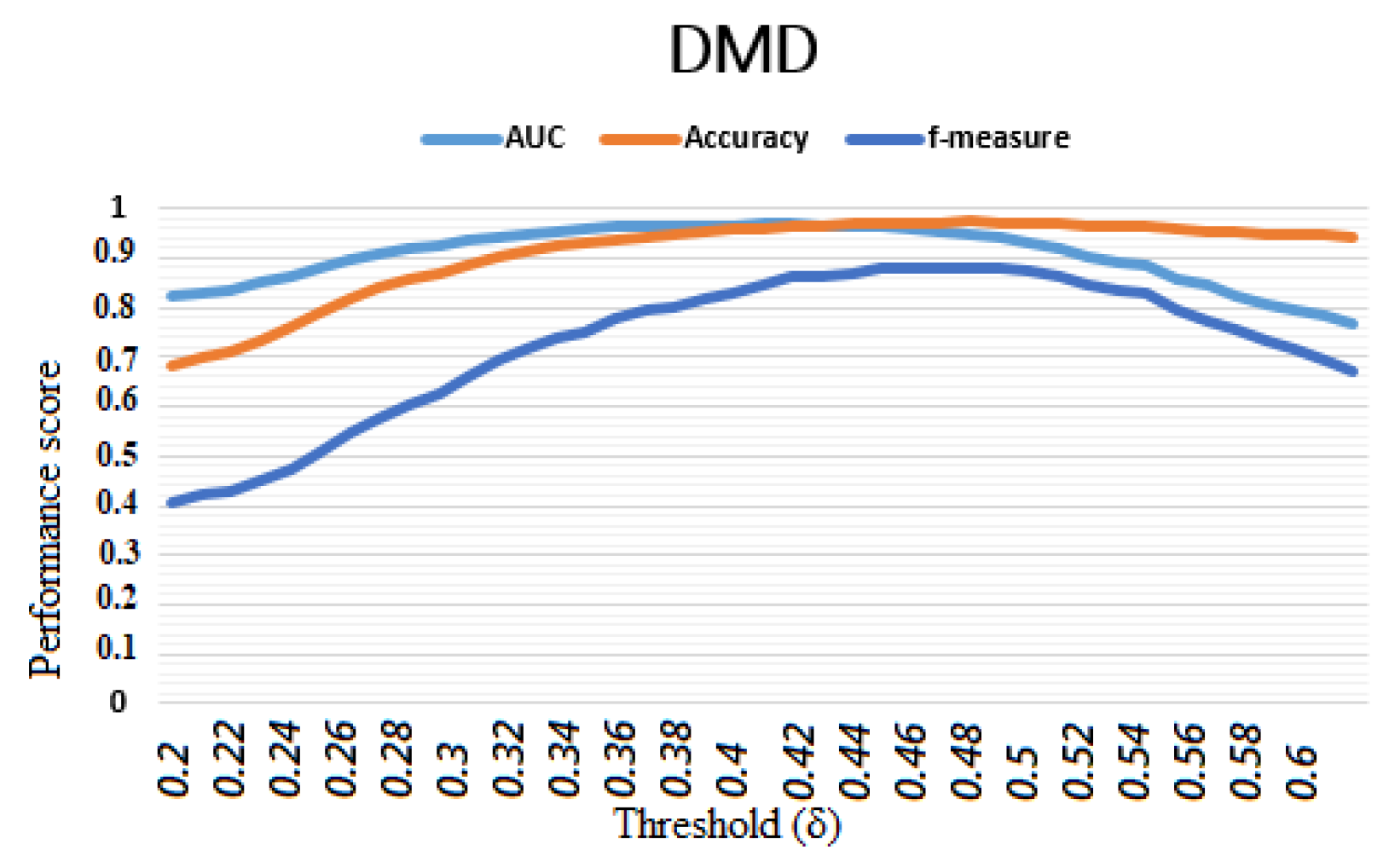
Wankhede et al. 2019) who used one hot encoding, which is known to multiply the variables and their processing time. In the CMB approach, the nominal variables are only processed by the decision function to optimise the processing time. On the other hand, the selection of the variables also contributes to optimising this processing time because 18 variables were significant to build a better model. Finally, still at the pre-processing level, the normalisation of the data allowed the scaling of the data to not only increase the performance, but also to stabilise the constructed model. The second advantage is the decision function, which deals directly with the nominal variables and contains only two parameters to be set in the optimisation process. This makes it very flexible and easy to optimise according to the training data, as we showed in Section 4.3. The model is globally fast with a processing time lower than the average given by the state-of-the-art methods while keeping almost the best performance scores. The high values of the accuracy, AUC and f 1 -measure with absolute deviations relatively less than five from each other prove that the model is less affected by the imbalance between the classes of the dataset compared to the works of (Krawczyk 2016; Marinakos and Daskalaki 2017). In addition, this function is easy to deploy in the real world and easily understood by bank marketers who do not necessarily have a great deal of knowledge of machine learning to use it or adapt it to new challenges. Although the CMB approach has many advantages, it is not without limitations related to our case study. One of them is related to the experimental protocol, which did not experiment with balancing the data by appropriate methods, such as SMOTE (Chawla et al. 2002), RAMO (Chen et al. 2010). The other is related to the use of certain variables, such as the call duration, which normally is only known after the call and therefore does not always reflect the reality in this database.

6. Conclusions

This paper presented and discussed the implementation on a Python platform of a class membership-based (CMB) approach to improve the prediction of call success in a commercial banking telemarketing campaign. The proposed approach provides a transparent process for preprocessing heterogeneous data and making optimal use of dummy variables that are often deleted or coded arbitrarily and/or in non-transparent ways during machine learning model building. The selection of meaningful features and normalisation not only improved performance, but also reduced processing time while stabilising the model for this data set. The use of a classification decision function directly incorporating the processing of categorical variables improved performance, reduced processing time, and furthermore, reduced the effects of class imbalance on the model performance and predictive risk. The constructed model was found to be more robust, stable, flexible and resistant to the effects of over-fitting. Its best performance reached 97.3%, 95.9% and 93.9% in terms of accuracy, AUC and f 1 -measure, respectively. Thus, the comparative analysis of our approach to classical machine learning algorithms and previous works showed that the CMB approach clearly overcomes the state-of-the-art works while offering, in addition, a relatively very low processing time. However, the approach is not yet suitable for other types of supervised machine learning problems, such as regression. Additionally, we have not yet experimented a combined approach with data- and time-variable balancing methods, which will be the focus of our future research.

Author Contributions

Conceptualization, S.C.K.T., Ş.C.G., H.T., P.N.M., M.N.M. and J.M.M.; methodology, S.C.K.T., Ş.C.G., H.T., P.N.M., M.N.M. and J.M.M.; software, S.C.K.T., Ş.C.G., H.T., P.N.M., M.N.M. and J.M.M.; validation, S.C.K.T., Ş.C.G., H.T., P.N.M., M.N.M. and J.M.M.; formal analysis, S.C.K.T., Ş.C.G., H.T., P.N.M., M.N.M. and J.M.M.; investigation, S.C.K.T., Ş.C.G., H.T., P.N.M., M.N.M. and J.M.M.; resources, S.C.K.T., Ş.C.G., H.T., P.N.M., M.N.M. and J.M.M.; data curation, S.C.K.T., Ş.C.G., H.T., P.N.M., M.N.M. and J.M.M.; writing—original draft preparation, S.C.K.T., Ş.C.G., H.T., P.N.M., M.N.M. and J.M.M.; writing—review and editing, S.C.K.T., Ş.C.G., H.T., P.N.M., M.N.M. and J.M.M.; visualization, S.C.K.T., Ş.C.G., H.T., P.N.M., M.N.M. and J.M.M.; supervision, S.C.K.T., Ş.C.G., H.T., P.N.M., M.N.M. and J.M.M.; project administration, S.C.K.T., Ş.C.G., H.T., P.N.M., M.N.M. and J.M.M.; funding acquisition, S.C.K.T., Ş.C.G., H.T., P.N.M., M.N.M. and J.M.M. All authors have read and agreed to the published version of the manuscript.

Funding

This research received no external funding.

Institutional Review Board Statement

Not applicable.

Informed Consent Statement

Not applicable.

Data Availability Statement

Not applicable.

Conflicts of Interest

The authors declare no conflict of interest.

Note

1
https://archive.ics.uci.edu/ml/index.php (accessed on 10 January 2018).

References

  1. Al-Garadi, Mohammed Ali, Amr Mohamed, Abdulla Khalid Al-Ali, Xiaojiang Du, Ihsan Ali, and Mohsen Guizani. 2020. A survey of machine and deep learning methods for internet of things (IoT) security. IEEE Communications Surveys & Tutorials 22: 1646–85. [Google Scholar] [CrossRef] [Green Version]
  2. Amini, Mohammad, Jalal Rezaeenour, and Esmaeil Hadavandi. 2015. A cluster-based data balancing ensemble classifier for response modeling in Bank Direct Marketing. International Journal of Computational Intelligence and Applications 14: 1550022. [Google Scholar] [CrossRef]
  3. Ballings, Michel, and Dirk Van den Poel. 2015. CRM in social media: Predicting increases in Facebook usage frequency. European Journal of Operational Research 244: 248–60. [Google Scholar] [CrossRef]
  4. Bhattacharyya, Siddhartha, Sanjeev Jha, Kurian Tharakunnel, and J. Christopher Westland. 2011. Data mining for credit card fraud: A comparative study. Decision Support Systems 50: 602–13. [Google Scholar] [CrossRef]
  5. Birant, Derya. 2020. Data Mining in Banking Sector Using Weighted Decision Jungle Method. In Data Mining-Methods, Applications and Systems. Rijeka: IntechOpen. [Google Scholar]
  6. Butcher, David, Xiangyang Li, and Jinhua Guo. 2007. Security challenge and defense in VoIP infrastructures. IEEE Transactions on Systems, Man, and Cybernetics, Part C (Applications and Reviews) 37: 1152–62. [Google Scholar] [CrossRef]
  7. Chawla, Nitesh V., Kevin W. Bowyer, Lawrence O. Hall, and W. Philip Kegelmeyer. 2002. SMOTE: Synthetic minority over-sampling technique. Journal of Artificial Intelligence Research 16: 321–57. [Google Scholar] [CrossRef]
  8. Chen, Sheng, Haibo He, and Edwardo A. Garcia. 2010. RAMOBoost: Ranked minority oversampling in boosting. IEEE Transactions on Neural Networks 21: 1624–42. [Google Scholar] [CrossRef]
  9. Cherif, Walid. 2018. Optimization of K-NN algorithm by clustering and reliability coefficients: Application to breast-cancer diagnosis. Procedia Computer Science 127: 293–99. [Google Scholar] [CrossRef]
  10. Cioca, Marius, Andrada Iulia Ghete, Lucian Ionel Cioca, and Daniela Gifu. 2013. Machine learning and creative methods used to classify customers in a CRM systems. Applied Mechanics and Materials 371: 769–73. [Google Scholar] [CrossRef]
  11. Elsalamony, Hany A., and Alaa M. Elsayad. 2013. Bank direct marketing based on neural network and C5. 0 Models. International Journal of Engineering and Advanced Technology (IJEAT) 2. [Google Scholar]
  12. Elsalamony, Hany A. 2014. Bank direct marketing analysis of data mining techniques. International Journal of Computer Applications 85: 12–22. [Google Scholar] [CrossRef]
  13. Farooqi, Rashid, and Naiyar Iqbal. 2019. Performance evaluation for competency of bank telemarketing prediction using data mining techniques. International Journal of Recent Technology and Engineering 8: 5666–74. [Google Scholar]
  14. Fawei, Torubein, and Duke T. J. Ludera. 2020. Data Mining Solutions for Direct Marketing Campaign. In Proceedings of the SAI Intelligent Systems Conference. Cham: Springer, pp. 633–45. [Google Scholar] [CrossRef]
  15. Feng, Yi, Yunqiang Yin, Dujuan Wang, and Lalitha Dhamotharan. 2022. A dynamic ensemble selection method for bank telemarketing sales prediction. Journal of Business Research 139: 368–82. [Google Scholar] [CrossRef]
  16. Ghatasheh, Nazeeh, Hossam Faris, Ismail AlTaharwa, Yousra Harb, and Ayman Harb. 2020. Business Analytics in Telemarketing: Cost-Sensitive Analysis of Bank Campaigns Using Artificial Neural Networks. Applied Sciences 10: 2581. [Google Scholar] [CrossRef] [Green Version]
  17. Govindarajan, M. 2016. Ensemble strategies for improving response model in direct marketing. International Journal of Computer Science and Information Security 14: 108. [Google Scholar]
  18. Grzonka, Daniel, Grażyna Suchacka, and Barbara Borowik. 2016. Application of selected supervised classification methods to bank marketing campaign. Information Systems in Management 5: 36–48. [Google Scholar]
  19. Huang, Xiaobing, Xiaolian Liu, and Yuanqian Ren. 2018. Enterprise credit risk evaluation based on neural network algorithm. Cognitive Systems Research 52: 317–24. [Google Scholar] [CrossRef]
  20. Ilham, Ahmad, Laelatul Khikmah, and Ida Bagus Ary Indra Iswara. 2019. Long-term deposits prediction: A comparative framework of classification model for predict the success of bank telemarketing. Journal of Physics: Conference Series 1175: 012035. [Google Scholar] [CrossRef]
  21. Karim, Masud, and Rashedur M. Rahman. 2013. Decision tree and naive bayes algorithm for classification and generation of actionable knowledge for direct marketing. Journal of Software Engineering and Applications 6: 196. [Google Scholar] [CrossRef] [Green Version]
  22. Kawasaki, Yoshinori, and Masao Ueki. 2015. Sparse Predictive Modeling for Bank Telemarketing Success Using Smooth-Threshold Estimating Equations. Journal of the Japanese Society of Computational Statistics 28: 53–66. [Google Scholar] [CrossRef] [Green Version]
  23. Khalilpour Darzi, Mohammad Rasoul, Majid Khedmati, and Seyed Taghi Akhavan Niaki. 2021. Correlation-augmented Naïve Bayes (CAN) Algorithm: A Novel Bayesian Method Adjusted for Direct Marketing. Applied Artificial Intelligence 35: 1–24. [Google Scholar] [CrossRef]
  24. Kotler, Philip, and Kevin Lane Keller. 2016. A Framework for Marketing Management. Boston: Pearson Education Ltd. [Google Scholar]
  25. Koumétio, Cédric Stéphane Tékouabou, Walid Cherif, and Silkan Hassan. 2018. Optimizing the prediction of telemarketing target calls by a classification technique. Paper presented at 2018 6th International Conference on Wireless Networks and Mobile Communications (WINCOM), Marrakesh, Morocco, October 16–19; pp. 1–6. [Google Scholar]
  26. Koumétio, Cédric Stéphane Tékouabou, and Hamza Toulni. 2021. Improving KNN Model for Direct Marketing Prediction in Smart Cities. In Machine Intelligence and Data Analytics for Sustainable Future Smart Cities. Cham: Springer, pp. 107–18. [Google Scholar] [CrossRef]
  27. Krawczyk, Bartosz. 2016. Learning from imbalanced data: Open challenges and future directions. Progress in Artificial Intelligence 5: 221–32. [Google Scholar] [CrossRef] [Green Version]
  28. Ładyżyński, Piotr, Kamil Żbikowski, and Piotr Gawrysiak. 2019. Direct marketing campaigns in retail banking with the use of deep learning and random forests. Expert Systems with Applications 134: 28–35. [Google Scholar] [CrossRef]
  29. Lahmiri, Salim. 2017. A two-step system for direct bank telemarketing outcome classification. Intelligent Systems in Accounting, Finance and Management 24: 49–55. [Google Scholar] [CrossRef]
  30. Lakshminarayan, Kamakshi, Steven A. Harp, and Tariq Samad. 1999. Imputation of missing data in industrial databases. Applied Intelligence 11: 259–75. [Google Scholar] [CrossRef]
  31. Leppäniemi, Matti, and Heikki Karjaluoto. 2008. Mobile marketing: From marketing strategy to mobile marketing campaign implementation. International Journal of Mobile Marketing 3: 1. [Google Scholar]
  32. Marinakos, Georgios, and Sophia Daskalaki. 2017. Imbalanced customer classification for bank direct marketing. Journal of Marketing Analytics 5: 14–30. [Google Scholar] [CrossRef]
  33. Miguéis, Vera L., Ana S. Camanho, and José Borges. 2017. Predicting direct marketing response in banking: Comparison of class imbalance methods. Service Business 11: 831–49. [Google Scholar] [CrossRef]
  34. Moro, Sérgio, Paulo Cortez, and Paulo Rita. 2014. A data-driven approach to predict the success of bank telemarketing. Decision Support Systems 62: 22–31. [Google Scholar] [CrossRef] [Green Version]
  35. Moro, Sergio, Raul Laureano, and Paulo Cortez. 2011. Using data mining for bank direct marketing: An application of the crisp-dm methodology. Paper presented at the European Simulation and Modelling Conference—ESM’2011, Guimaraes, Portugal, October 24–26; pp. 117–21, EUROSIS-ETI. [Google Scholar]
  36. Moro, Sérgio, Paulo Cortez, and Paulo Rita. 2015. Using customer lifetime value and neural networks to improve the prediction of bank deposit subscription in telemarketing campaigns. Neural Computing and Applications 26: 131–39. [Google Scholar] [CrossRef]
  37. Moro, Sérgio, Paulo Cortez, and Paulo Rita. 2018. A divide-and-conquer strategy using feature relevance and expert knowledge for enhancing a data mining approach to bank telemarketing. Expert Systems 35: e12253. [Google Scholar] [CrossRef] [Green Version]
  38. Mustapha, SMFD Syed, and Abdulmajeed Alsufyani. 2019. Application of Artificial Neural Network and Information Gain in Building Case-based Reasoning for Telemarketing Prediction. International Journal of Advanced Computer Science and Application 10: 300–6. [Google Scholar] [CrossRef]
  39. Pedregosa, Fabian, Gaël Varoquaux, Alexandre Gramfort, Vincent Michel, Bertrand Thirion, Olivier Grisel, Mathieu Blondel, Peter Prettenhofer, Ron Weiss, Vincent Dubourg, and et al. 2011. Scikit-learn: Machine learning in Python. The Journal of Machine Learning Research 12: 2825–30. [Google Scholar]
  40. Rust, Tobias, Daniel Bruggemann, Wilhelm Dangelmaier, and Dominik Picker-Huchzermeyer. 2010. A Method for Simultaneous Production and Order Planning in a Cooperative Supply Chain Relationship with Flexibility Contracts. Paper presented at 2010 43rd Hawaii International Conference on System Sciences, Koloa, HI, USA, January 5–8; pp. 1–10. [Google Scholar] [CrossRef]
  41. Selma, Mokrane. 2020. Predicting the Success of Bank Telemarketing Using Artificial Neural Network. International Journal of Economics and Management Engineering 14: 1–4. [Google Scholar]
  42. Sihombing, Ester Hervina, and Nasib Nasib. 2020. The Decision of Choosing Course in the Era of Covid 19 through the Telemarketing Program, Personal Selling and College Image. Budapest International Research and Critics Institute (BIRCI-Journal): Humanities and Social Sciences 3: 2843–50. [Google Scholar] [CrossRef]
  43. Tekouabou, Stéphane Cédric Koumetio, Walid Cherif, and Hassan Silkan. 2019. A data modeling approach for classification problems: Application to bank telemarketing prediction. Paper presented at 2nd International Conference on Networking, Information Systems & Security, New York, NY, USA, March 27–29; pp. 1–7. [Google Scholar]
  44. Tekouabou, Stéphane Cédric Koumetio, Sri Hartini, Zuherman Rustam, Hassan Silkan, and Said Agoujil. 2021. Improvement in automated diagnosis of soft tissues tumors using machine learning. Big Data Mining and Analytics 4: 33–46. [Google Scholar]
  45. Thakar Pooja, Mehta Anil, and Sharma Manisha. 2018. Robust Prediction Model for Multidimensional and Unbalanced Datasets. International Journal of Information Systems & Management Science 1: 2. [Google Scholar]
  46. Tripathi, Diwakar, Damodar Reddy Edla, Venkatanareshbabu Kuppili, Annushree Bablani, and Ramesh Dharavath. 2018. Credit Scoring Model based on Weighted Voting and Cluster based Feature Selection. Procedia Computer Science 132: 22–31. [Google Scholar] [CrossRef]
  47. Turkmen, Egemen. 2021. Deep Learning Based Methods for Processing Data in Telemarketing-Success Prediction. Paper presented at 2021 Third International Conference on Intelligent Communication Technologies and Virtual Mobile Networks (ICICV), Tirunelveli, India, Frbruary 4–6; pp. 1161–66. [Google Scholar] [CrossRef]
  48. Vafeiadis, Thanasis, Konstantinos I. Diamantaras, George Sarigiannidis, and Konstantinos C. Chatzisavvas. 2015. A comparison of machine learning techniques for customer churn prediction. Simulation Modelling Practice and Theory 55: 1–9. [Google Scholar] [CrossRef]
  49. Vajiramedhin, Chakarin, and Anirut Suebsing. 2014. Feature selection with data balancing for prediction of bank telemarketing. Applied Mathematical Sciences 8: 5667–72. [Google Scholar] [CrossRef]
  50. Yan, Chun, Meixuan Li, and Liu Wei. 2020. Prediction of bank telephone marketing results based on improved whale algorithms optimizing S_Kohonen network. Applied Soft Computing 92: 106259. [Google Scholar]
  51. Yu, Lei, and Huan Liu. 2003. Feature selection for high-dimensional data: A fast correlation-based filter solution. Paper presented at 20th International Conference on Machine Learning (ICML-03), Washington, DC, USA, August 21–24; pp. 856–63. [Google Scholar]
  52. Wankhede Prabodh, Singh Rohit, Rathod Rutesh, Patil Jayesh, and Khadtare TD. 2019. Improving Prediction of Potential Clients for Bank Term Deposits using Machine Learning Approaches. International Research Journal of Engineering and Technology 6: 7101–4. [Google Scholar]
Figure 1. The global process of a predictive classification system with the CMB approach.
Jrfm 15 00269 g001
Figure 2. Flowchart of the classification steps of the CMB algorithm.
Jrfm 15 00269 g002
Figure 3. Illustration of our experimental protocol.
Jrfm 15 00269 g003
Figure 4. Variation in performance according to the decision threshold ( δ ).
Jrfm 15 00269 g004
Figure 5. The cumulative gain curve of the CMB model (Class 0 is for “yes” label and class 1 is for “no” label).
Jrfm 15 00269 g005
Figure 6. Comparison of CMB models’ performance with other common machine learning models.
Jrfm 15 00269 g006
Figure 7. Comparison of model complexity in terms of average minimum processing time.
Jrfm 15 00269 g007
Table 1. Summary of the relevant papers dealing with direct bank telemarketing prediction using machine learning. SRAP = Scientific Research an Academy Publisher; CBWDJ = Class-based weighted decision jungle, JSCS = Japanese Society of Computational Statistics.
Ref.Year Nb f ToolsAlgorithmsMetricsBest Score (%)PublisherType
Feng et al. (2022)202221PythonMETA-DES-AAPAcc, AUC89.39; 89.44ElsevierArticle
Koumétio and Toulni (2021)202113Pythonimproved KNNAcc, AUC, f 1 96.91SpringerChapter
Yan et al. (2020)202021-S_Kohonen networkAcc80ElsevierArticle
Ghatasheh et al. (2020)202021-CostSensitive-MLPAcc84.18MDPIArticle
Selma (2020)202021-ANNAcc; f 1 98.93; 95.00WasetArticle
Birant (2020)202021-CBWDJ(Acc; Arec; Rec)(92.70; 84.92; 75.93)IntechOpenChapter
Tekouabou et al. (2019)201921PythonDT C5.0Acc, Prec, Rec, f 1 100ACMConf
Farooqi and Iqbal (2019)201921WEKADT J48Acc, Spe, Sen, prec, AUC, f 1 91.2; 95.9; 53.8; 62.7; 88.4; 58IJRTEArticle
Mustapha and Alsufyani (2019)201917-ANNInfo Gain, Entropy-The SAIArticle
Ilham et al. (2019)201921RapidMinerSVMAcc, AUC97.7; 92.5IOPChapter
Ładyżyński et al. (2019)201921H2ORF, DLprc, rec ElsevierArticle
Koumétio et al. (2018)201818RapidMinerDT C4.5Acc, f 1 87.6; 81.4IEEEConf
Moro et al. (2014)201422R/rminerLR, DT, NN, SVMAUC; ALIFT80.0; 70.0ElsevierArticle
Vajiramedhin and Suebsing (2014)20148-C4.5Acc, AUC92.14; 95.60HikariArticle
Elsalamony (2014)201417SPSSMLPNN, TAN, LR, C5.0Acc, Sens, Spec90.49; 62.20; 93.12FCSArticle
Karim and Rahman (2013)201321WEKANB; C4.5Acc, Prec, AUC93.96; 93.34; 87.5SRAPArticle
Elsalamony and Elsayad (2013)201318-BC, RF, SC, GB (C5.0)Acc; AUC; Kappa96.11; 99.3; 91.70SRPArticle
Moro et al. (2011)201129R/rminerNB; DT; SVMAUC; ALIFT93.8; 88.7EUROSIS-ETIArticle
Table 2. Example of the initial dataset.
Inst. f 1 f 2 f 3 f 4 Label
I 1 59marriednoregularno
I 2 39singleyesvery regularyes
I 3 59marriednoirregularno
I 4 41divorcednoUnknownyes
I 5 44marriednoirregularyes
Table 4. Normalised data.
Inst. f 1 f 2 f 3 f 4 Label
I 1 1married00.50
I 2 0single111
I 3 1married000
I 4 0.1divorced00.51
I 5 0.25married001
Table 5. Reduced table.
f 1 f 2 f 3 f 4
C j 0.980.80.410.33
C n o 59married00.5
C y e s 41.33single; divorced0.331
Table 6. Combining results of CMB on four DMD dataset.
ModelAUCAccuracy f 1 -MeasureProcessing Time (s)
basic78.1%90.0%57.9%0.81
with FN76.9%89.9%56.8%0.45
with FNW95.9%97.3%93.2%0.52
Table 7. Comparison of the best performances of previous work.
AccAUC N f Best ModelYear
Feng et al. (2022)89.39%89.44%21META-DES-AAP2022
Moro et al. (2011, 2014)NA0.93822ANN2014
Elsalamony and Elsayad (2013); Elsalamony (2014)90.09%NA17DT(C4.5)2014
Vajiramedhin and Suebsing (2014)92.14%21NADT(C4.5)2014
Grzonka et al. (2016)89.4%NA8Random Forest2016
Karim and Rahman (2013)93.96%0.9334NADT(C4.5)2013
Lahmiri (2017)71%0.5918Two-stage system2017
Koumétio et al. (2018)69.1%0.5518DT2018
Tekouabou et al. (2019)100%-21DT2019
Farooqi and Iqbal (2019)91.2%-21DT2019
Selma (2020)98.93%0.9521ANN2020
Koumétio and Toulni (2021)96.91%95.912KNN2021
CMB approach97.3%95.918CMB2022
Publisher’s Note: MDPI stays neutral with regard to jurisdictional claims in published maps and institutional affiliations.

