1. Introduction
The global financial crisis of 2008, also known as the subprime mortgage crisis, is classified as the world’s worst crisis since the Great Depression of 1930. The initial collapse of Lehman Brothers triggered a cascading effect of failures, thus exposing the high systemic risk embedded in a highly interrelated and interdependent banking network. Systemic risk in a banking system is defined as the risk of destabilization of the whole system, caused by the failure of a single or a small set of banking institutions. The collapse of Lehman Brothers threatened the viability of many other large financial institutions. The ones that eventually survived received significant subsidies (through bailout programs) under the Troubled Assets Relief Program (TARP) implemented by the government. The same was not true for a set of smaller institutions that were left to collapse.
Historically, following each banking crisis, a series of acts were introduced aiming to stabilize the banking system and avoid a future reoccurrence of a crisis. The Banking Act of 1933, commonly known as the Glass–Steagall Act, was signed by President Franklin Roosevelt as an attempt to restore confidence in the U.S banking system. The bill was designed to reform the banking system by imposing a dichotomy between commercial and investment banking in order to reduce risk. It also intended to allow for a safer and more effective use of banks’ assets, to regulate interbank control, and prevent banks from conducting speculative operations. This boosted disintermediation, which is the practice of financing directly from capital markets without the intermediation of banks, thus reducing the banks’ share in total financing. As a result, banking institutions pursued the abolishment of the Glass–Steagall Act, and several decades later, the U.S Congress passed the Gramm–Leach–Bliley Act of 1999, which was signed into law by President Clinton. The Gramm–Leach–Bliley Act waved the preexisting barriers in financial markets; hence, banking institutions were again free to engage in security trading and insurance contracts that helped them increase their market share. This newly gained freedom, and the inevitable fierce competition with non-banking institutions, led to the rapid development in the markets of new and diverse financial instruments. In effect, the liberalization of the banking sector led to a significant increase in systemic risk, as banks have since been exposed to investment and other types of risk. Many analysts believe that the 2008 financial crisis is directly linked to the imposition of the Gramm–Leach–Bliley Act. The lack of separation between commercial and investment banking activities, allows financial institutions to be involved in security trading, not only for their customers, but also for themselves, a practice that exposes common depositors to high market risk.
After the 2008 financial crisis, the Obama administration enacted the Dodd–Frank Wall Street Reform and Consumer Protection Act in 2010, in an attempt to minimize systemic risk, enforce financial sector’s transparency and accountability, and implement rules for consumers’ protection; however, the provisions of the Dodd–Frank Act did not include the strict separation between commercial and investment banking, and thus, it cannot fully minimize such risk in the banking sector.
It is essential for the regulators to swiftly pinpoint incidents of bank distress. A prompt identification of instances of increased systemic risk can help minimize the policy reaction time. This can help minimize the contagion and defuse the propagation of a potential financial crisis; thus, an effective and continuous monitoring of financial institutions is necessary for the maintenance of a solvent and stable banking system. Increased supervision and strict regulation of the banking system is also required by the new Basel Accord (Basel III) by the Basel Committee on Banking Supervision, introduced in the U.S. in 2013, and implemented in 2018. Recently,
Durana Pavol et al. (
2021) revealed the impact of bankruptcy risk on the level of earnings management in the life cycle stages.
According to the new Basel Accord framework, the regulatory authorities are responsible for: (a) implementing extensive supervision of the banking system, and (b) mitigating the effects of possible crises and limiting contagion. A significant concern, apart from finding the appropriate monitoring tools, is the appointment of such a regulatory authority. A great deal of research supports the idea that supervision of the entire banking system should be vested to a single authority.
Vives (
2001) and
Blinder (
2010) support the idea that a single authority can (a) establish credible systems, (b) achieve economies of scale, and (c) reach financial stability by taking advantage of the economies of scale between the Lender of Last Resort (LOLR) facility, supervision, and monetary policy.
Boyer and Ponce (
2012) support the idea that a single supervisory authority preserves a more effective supervision of the banking system than the one achieved by multiple authorities. Following the idea that a single authority can competently optimize the supervision of the entire banking system by providing a timely and efficient intervention, in October 2012, E.U. leaders decided to assign the supervision of the whole European banking network to a single authority, the ECB.
In this paper, we introduce the multivariate Threshold–Minimum Dominating Set (mT-MDS) methodology, and then use it to group the banking network in neighborhoods according to their financial health. The mT-MDS is an extension of the T-MDS methodology that is especially designed to treat multivariate networks, since the T-MDS can handle only univariate ones. The methodology creates a multilayered network and distills the multivariate information in one binary network using a Boolean operator. The multilayered network is built using the variables that were identified in
Gogas et al. (
2018) for banking bankruptcy forecasting. Τhe empirical results reveal that the neighborhoods efficiently classify solvent and failed institutions. We propose the mT–TMDS method, as an auxiliary monitoring mechanism and an extra layer on banking supervision.
The rest of the paper is organized as follows. In
Section 2, we present a literature review of studies related to ours. In
Section 3, we present the multivariate T-MDS model. In
Section 4, we present our dataset, and in
Section 5,we provide a brief discussion and draw the conclusions.
2. Literature Review
Systemic risk is spread through the multiple interrelations between financial institutions in a banking network. A simple, concise, and efficient way to model this system is by using a complex network representation; each bank is represented by a node and the interrelation between two banks is represented by an edge linking them. The theory of complex networks provides a set of tools that are able to examine the structure of economic networks.
Mantegna (
1999) and
Hill (
1999) were the first to apply complex networks in economic systems. More specifically,
Mantegna (
1999) uses the MST in his attempt to study the hierarchical structure of the New York Stock Exchange, whereas
Hill (
1999) compared price levels across countries using the same methodology. Some closely related papers to
Mantegna (
1999) and
Hill (
1999), are
Tumminello et al. (
2007),
Bonanno et al. (
2004),
Lyocsa et al. (
2012),
Tabak et al. (
2010),
Onnela et al. (
2004),
Kumar and Deo (
2012), and
Sandoval (
2012). The application of complex networks in economics, and particularly, in banking, has grown expeditiously during the last few years. There are several studies that examine the risk of contagion.
The seminal paper of
Allen and Douglas (
2000) investigates the cascading effect of a banking crisis on a network of regions or economic sectors. The authors showed that two cases are resilient to a liquidity shock: (a) the case of a complete interbank market (i.e., a market where every bank is connected to all the other banks in the network) and (b) an incomplete interbank market with a low degree of interconnectedness. Conversely, in the case of an incomplete interbank market with a high degree of interconnectedness, the liquidity shock may spread to the whole network. Similar conclusions are drawn from the studies of
Leitner (
2005) and
Gai and Kapadia (
2010), where the results revealed that as the network becomes denser, systemic risk drops, and the influence of an institution’s default is negligible as the losses of the failed institution will be spread and engrossed from the rest of the institutions in the network.
Several studies analyze the topology of real-word economic and financial networks. Their aim is to explore the roots of systemic risk and how this risk spreads in a banking network. The studies of
Fagiolo et al. (
2009),
Inaoka et al. (
2004),
Iori et al. (
2006),
Iori et al. (
2008),
Nacher and Akutsu (
2012),
Huang et al. (
2008) and
Angelini et al. (
1996) draw the conclusion that the structure of banking networks is characterized as scale-free
1 and core periphery
2. The distinct feature of these two structures is that all networks are formed from a small number of hub banks, whereas the rest of the banks are periphery banks. Hub banks are highly interconnected, whereas, on the other hand, periphery banks are not. In these networks, the hub banks determine the system’s robustness. If the hub banks are not affected by a shock in the economy, then the system is not exposed to systemic risk and the network remains healthy. On the contrary, if a hub bank suffers a shock, the crisis may be directly spread to a large part of the network, thus increasing the risk of a system failure. The only way to stop the contagion in such a case, is by supporting the hub banks with sufficient funds.
In order to examine the origins of systemic risk in depth, a number of papers analyze the topology of real word networks in an effort to identify their features.
Minoiu and Reyes (
2011), analyze the topology of the global banking network, formed of financial flows during and after periods of financial stress. The findings show that a number of structural breaks in the network indicate the waves of capital flows before and after crises. A network’s centrality falls at the beginning of and after a debt crisis. In the study of
Tabak et al. (
2014), the authors introduce the directed clustering coefficient as a measure of systemic risk in complex networks. The results reveal that the network is not exposed to systemic risk, and more specifically, the clustering coefficient and domestic interest rates reveal negative correlation; as interest rates increase, the banks decrease their exposure to the system.
Thurner et al. (
2003), examine the impact of a network’s structure on the wealth of the economy, concluding that a highly connected network is more stable since it is not exposed to large wealth changes.
Hoggarth et al. (
2002) assesses the impact of a banking crisis in developed and emerging countries. The study concludes that developed countries experience larger losses on average during crisis periods compared with emerging countries.
Kuzubas et al. (
2014) use centrality measures such as betweenness centrality, closeness centrality, and Bonacich’s centrality, in order to assess the network’s connectivity and identify the systemically important institutions. The results reveal that the centrality measures are adequate for the identification and the observance of systemically important financial institutions.
Furthermore, there are studies using the balance sheet-based technique to explore and evaluate the interrelations of banking institutions and their level of influence in the overall banking system. These studies test the influence of credit relations in different banking systems. Their aim is to explore how mutual claims between banks can affect the propagation of contagion.
Upper and Worms (
2004) study the German banking system,
Cocco et al. (
2009) analyze the Portuguese banking system,
Wells (
2004) explores the U.K. interbank market,
Boss et al. (
2004) study the Austrian interbank market,
Furfine (
2003) studies the U.S. banking system,
Degryse and Nguyen (
2004) tests the Belgian interbank market, and
Sheldon and Maurer (
1998) study the Swiss banking system. The results of the above studies overlap with one another, and they reveal that the default of a single institution is not capable of triggering the collapse of the entire system, though it is able to influence a quite small part of the network. All studies reach the same conclusion: banking systems are robust even if a single institution fails. Finally,
Chan-Lau (
2010) also uses a balance sheet-based approach to examine whether the financial crisis of 2008, which was triggered by an institution’s failure and spread to the largest part of the world, was the aftermath of the institutions’ interbank exposure and their externalities with too-connected-to-fail institutions. The results reveal that when shocks in the network jeopardize banks’ solvency, they can be characterized as sources of financial contagion worldwide.
We presented a large collection of papers focused on measuring the robustness of a banking network and its exposure to systemic risk. Our approach differs as it is oriented toward the optimization of network monitoring. Μore specifically, we propose the introduction of a new monitoring layer to the existing systems for bank supervision. In this layer, the regulator will identify a reduced version (small subset) of the initial network that: (a) contains an adequate amount of the total information and (b) is easier to monitor and analyze. We merge these two targets into one under the term
representation goal. We investigate the interrelations between banking institutions using tools from the complex networks theory, and more specifically, graph theory. In
Gogas et al. (
2016) we introduced a two-step methodology termed T-MDS for the identification of a small subset of nodes that are able to represent the entire network. In our setup, the nodes are the economic entities (banks), and the edges define temporal similarity as described by the correlation. We showed that the T-MDS banks can be used as distress sensors for the whole banking network.
3. Methodology
In this paper, we introduce the multivariate Threshold–Minimum Dominating Set (mT-MDS), a multivariate extension of the T-MDS. The mT-MDS shares the same goals with the T-MDS, though it works in a multivariate environment. Indeed, the main limitation of the T-MDS methodology lies in its univariate design; the network is built based on only one variable, and the representation goal may be unreachable in such a poor environment in terms of information. Banking interconnections are complex, and they are better described by more than one variable. With this need in mind, here, we introduce and employ the multivariate T-MDS. We begin with some basic concepts of graph theory.
Definition 1. A graph G consists of a collection V of nodes and a collection Ε of edges, for which we write G = (V, E). An edge eij ⋲ E is said to join the nodes i and j. The structure can be extended by assigning numerical values (often called weights) to each edge representing quantitative relations vij.
To fully comprehend the methodology and the explanation of the empirical results, the following key concepts must be defined:
Isolated node is a node that is not connected to any other node in the network.
Interconnected node is any node that is connected to at least another node in the network.
In our experiments, the nodes represent economic entities (banks), the edges represent the existence (or not) of a relation (similarity) between two nodes, and the weights of the edges measure the relation between the two nodes (in our tests we calculated the temporal similarity between nodes using the Pearson’s correlation coefficient r). To identify the smallest subset of nodes that can represent the whole network we will use the notion of a ‘dominating set’.
Definition 2. A dominating set of a graph G is a subset of nodes DS ⊆ V such that every node v ∉ DS is directly connected to at least one member of the DS. The members of the DS are called dominant nodes.
Moreover, if we identify a dominating set of a graph, any node of the graph is either (a) a dominant node or (b) a node directly connected to a dominant node. This is a particularly important property to us, since it means that, given that the edges of a graph describe a high similarity between the nodes, the whole network can be represented by the dominating set. Indeed, by the definition of DS, every non-dominant node is directly connected with at least one dominant node by an edge that describes a high similarity. The nodes directly connected with a dominant node form the neighborhood of the dominant node. The dominant node of a neighborhood will serve as the representative node of the group.
A network can have many DSs. The ones with minimum cardinality are called Minimum Dominating Sets (MDS). The MDS can be identified through a minimization process:
First, one must define the variables
representing the nodes’ membership to the MDS (1 describes the dominance and 0 describes the non-dominance of a node). These variables in vector form are
The Minimum Dominating Set is identified by minimizing:
subject to
where
represents the set of adjacent nodes of node
The assumption is straightforward: the node
i can be (a) a node of the MDS (
. or (b) adjacent to at least a MDS node (
. In any case, the l.h.s of the constraint is equal to or greater than 1. The imposed constraint ensures that every node of the network will be represented from the MDS subset.
In real data networks, all the edges may not describe a high similarity between its endpoint nodes. Couples of low correlated entities may exist in the network. These low correlation edges are undesired in the identification of the MDS; we wish to monitor every neighborhood through its dominant node, and this is only achieved if the edges describe a high correlation; therefore, we add a thresholding step on the correlation level marked as weight on the edges, thus eliminating the low correlation ones from the network. After this step, all the edges depict the desired representation goal, which is high similarity.
During the thresholding, isolated nodes may appear in the network. Nodes with all weight edges below the selected threshold become isolated. Even if the focus of this study is the representation of the interconnected banks, the isolated banks are important as well since they are the members of the banking network that exhibit unique idiosyncratic behavior. Any isolated node can only be represented by itself and is a member of the T-MDS by definition.
This methodology was introduced in
Gogas et al. (
2016), termed as the Threshold–Minimum Dominating Set (T-MDS) and defined with the following steps:
Preprocessing: Create the network using Pearson’s correlation coefficient of the selected variable.
Step 1. Apply a threshold on the weights and eliminate the edges with weights less than the threshold.
Step 2. Identify the MDS nodes on the resulting network.
We claim that every dominant node in the T-MDS can be perceived as a sensor for its directly connected neighborhood nodes, since they are connected with edges that survived the thresholding step (i.e., they are highly similar/correlated). Thus, all the nodes in a neighborhood are expected to exhibit a similar behavior. In our empirical section, we examined the solvency of the banking institutions. If the dominant node is expected to fail (or not), so are the neighboring nodes. Empirical results in
Gogas et al. (
2016) backed this theory in the univariate T-MDS methodology.
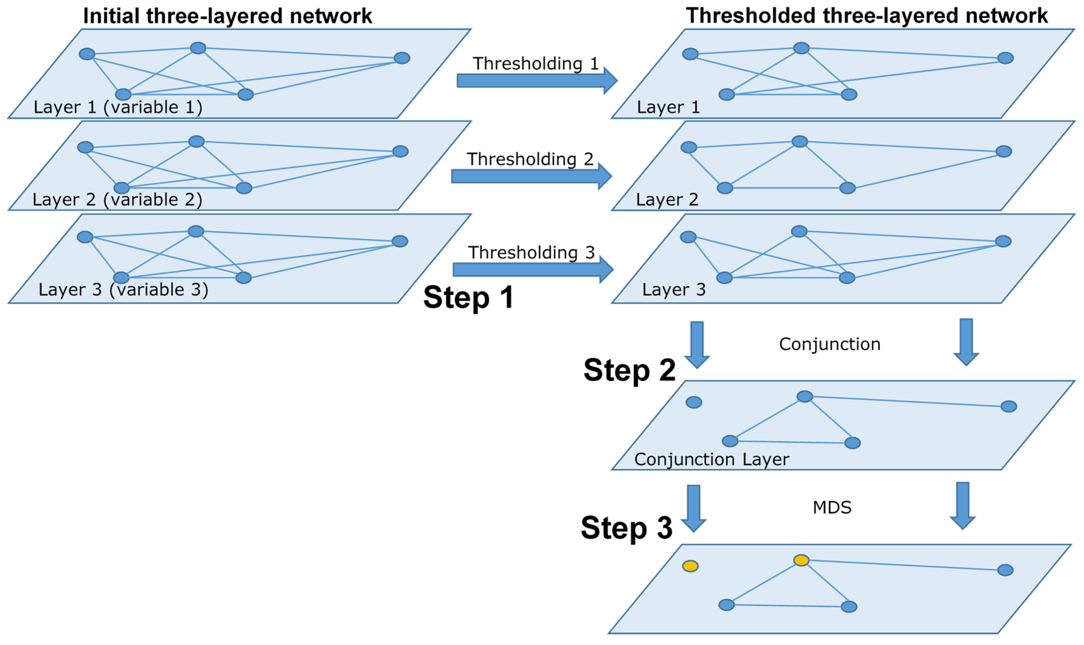
In this paper, we extend the T-MDS concept to multiple variables. We call it a multivariate Threshold–Minimum Dominating Set (mT-MDS), which is the three-step methodology for the identification of the network’s most representative nodes in a multilayered network:
Preprocessing: For each variable, create the correlation-based network. The network is a layer in the multilayered framework.
Step 1: Impose a threshold in every layer to eliminate the low correlation edges, which produces thresholded layers. The threshold level may vary across layers.
Step 2: For every couple of nodes, combine the edge information from all layers using an operator. In our experiments, we used the conjunction Boolean operator. An edge is created when an edge exists between the two nodes in every layer. This step results in the creation of a single unweighted binary network.
Step 3: Identify the MDS.
In
Figure 1 we graphically depict a representation of the mT-MDS.
Initially, there is an edge between every node (regardless of the correlation level). In Step 1, the thresholding eliminates the low correlation edges in each layer of the network. After this point, the edges have no weights and describe the high correlation of its endpoints. Its absence means the opposite. The information of all layers is combined in a single binary network in Step 2, through the Boolean conjunction
3. An edge in the resulting network describes nodes that are highly correlated in all layers, and thus, for every variable. The final step is the identification of the dominant nodes in the network and their respective neighborhoods. In
Section 5, we will show the superiority of this method over the simple T-MDS.
3.1. Discussion on the Methodology
In this section, we would like to address two interesting issues regarding the mT-MDS:
Is the proposed methodology affected by the correlation of the variables?
In the case of a highly correlated multivariable network, the univariate networks in each layer have a similar structure (the same edges survive the thresholding step). Thus, the same edges appear in most of the layers after thresholding, and these edges can survive the conjunction step. The more correlated the variables, the more the final network is similar to the univariate ones. The opposite is true when the variables are not highly correlated. The more uncorrelated the variables, the more distinct the final network will be compared with the univariate ones.
Can we replace the multilayered network by adopting a unique composite variable in a uni-layered network instead?
In the past, we tested this option using the z-scores, but we abandoned it for two main reasons. The first reason is flexibility. The multivariate network model offers the ability to test a different threshold in each layer. In this setting, when there are problems where the variables are not equally important to the final goal, we may choose a lower threshold for the unimportant variables and a stricter one for the important ones. This is a feature that is lost when we combine many variables into one. The second reason is interpretability. The univariate networks are interpretable, since the edges are created using true variables, which are observable by the network supervisors. The same is not true when these variables are hidden in a composite variable of any kind.
3.2. The Data
The examined period spans from 2006Q1 to 2010Q3, a period that includes a major financial crisis where many banks failed. We collected quarterly data from the databank of the Federal Deposit Insurance Corporation (FDIC), and they include 570 US banks. Of these banks, 429 were solvent and 141 failed. The 141 failed institutions represent the total number of banks that failed during the 2010–2011 period and they have available data for all the studied quarters. We also collected data from the 429 largest—in terms of total assets—solvent banks, to maintain a 3:1 ratio between solvent and failed banks.
Gogas et al. (
2018) created a machine learning-based forecasting model for bank failures for the period 2007–2013 that produces a remarkably high overall accuracy, reaching 99.22%. Their model selected from an initial extensive list only two variables: (a) Tier 1 (core) risk-based capital over total assets (T1CRC); and (2) total interest expense over total interest income (TIE). The same two variables were used in the empirical section of our paper, since our goal is to test the presented methodology on banking solvency.
Tier 1 (core) risk-based capital over total assets includes disclosed reserves and equity capital and provides a measure of a bank’s capital adequacy. It is a significant ratio that is considered as a proxy of a bank’s financial strength. It provides a relative measure of the number of financial losses a bank can absorb without requiring new capital injections. Whenever a recapitalization is needed, the new capital can either be added through a common increase of share capital, or in times of crisis, through a bail-out or a bail-in program. Total assets measure the absolute size of a bank. In times of economic expansion, banks tend to augment their assets mainly by issuing new loan facilities; in times of declining economic activity, they reduce their lending, and as a result, total assets and their balance sheet is reduced. A direct way that a crisis propagates through the banking system is via interbank loans. A troubled bank that used interbank lending to augment its balance sheet and provide more loan facilities, is unable to repay its financial obligations to other banks, and thus, the total assets of the lending banks take a hit. In general, banks with higher T1CRC ratios are associated with lower probability of default (
Gogas et al. 2018). The total interest expense over the total interest income (TIE) ratio provides a proxy of a bank’s operational efficiency from its core business (i.e., pooling funds and lending). The nominator includes all interest paid by the bank for its interest-bearing liabilities, and the denominator includes all interest earned on any type of lending from the assets’ side of the balance sheet. An increasing TIE ratio reflects a declining gross profit margin.
4. Empirical Results
Trivially, a network combining two variables is, information-wise, richer than a univariate one; however, the combination of the two variables through a logical conjunction may result in a significant loss of information
4, rendering the multivariate network appealing in theory, but not in practice. In this section, we will compare the univariate networks to the multivariate ones, and show that the information loss is negligible, and the multivariate network neighborhoods better portray the banking solvency.
4.1. Comparison between the T-MDS and mT-MDS Networks
In the univariate T-MDS, we create two networks: one based on the Tier 1/total asset variable, and one based on the total interest expense/total interest income variable. In the multivariate T-MDS, we create a layer for each variable (in a multilayered framework) and then combine them in one binary network (without weights). In every case, the threshold level will be set at 0.8. The composition of the univariate networks after thresholding are shown in
Table 1 and
Table 2, and the composition of the multivariate network after thresholding and logical conjunction is shown in
Table 3.
The Tier1/total asset-based network after thresholding retains 446 of the nodes interconnected (78.3%), whereas 124 of the nodes (21.7%) are isolated from the rest of the network. The interconnected part is clustered in 53 neighborhoods (47 with a solvent dominant node and 16 with a failed one).
The total interest expense/total interest income-based network is almost unaffected by the thresholding step; only 3 nodes became isolated. The 567 interconnected nodes are represented by 11 dominant nodes (5 solvent and 6 failed ones).
The multilayered network refines the univariate layers to a binary one through the logical conjunction. Thus, for an edge to “survive” the conjunction step, it should appear in every layer of the multilayered network. Consequently, the number of edges in the resulting binary network can be, as a maximum, as many as in the layer with the fewest edges. The same is true for the number of interconnected nodes. Thus, in our case, the upper limit of the interconnected part in the multivariate case is 446 nodes (the interconnected part in the thresholded Tier 1/total asset network, which is the smallest interconnected part). The combination of the univariate layers in a multivariate one results in 413 interconnected nodes clustered in 72 neighborhoods and 157 isolated ones. The multivariate thresholded network has 33 (5.8%) fewer interconnected nodes than the Tier 1/total assets univariate network. Next, we will demonstrate that this did not affect the results quantitatively or qualitatively.
4.2. Comparison of the T-MDS and mT-MDS Clustering
In this paper, our main goal is to create a monitoring tool that will be able to swiftly examine the health state of the entire banking network (all neighborhoods) using only information from the representative nodes (dominant nodes). Such a tool would be fast, easy to use, and low-cost. Thus, it could be used by the supervising authority as an auxiliary monitoring system for the health of the banking sector.
Ideally, we would like to be able to label every node of a neighborhood, based on the state of the dominant node, as solvent or failing. It must be noted here that a node may belong to more than one neighborhood. Consequently, in some cases, a node may be labeled as both solvent and failed. We call these nodes “fuzzy”. The fuzzy nodes have the disadvantage that they introduce uncertainty into our monitoring tool. We are unable to forecast the fate of a fuzzy node.
The misclassification of our system (nodes that belong to a single neighborhood and thus have one label, but it is the wrong one) may create two distinct cases—false alarms or missed failures. Obviously, the costs of a false alarm with regard to the efficient monitoring of the banking system is far less than a missed failure (i.e., identifying a bank as healthy while it is actually failing). The latter may potentially have cascading effects due to contagion, which would subsequently cause systemic risks to the banking sector; however, we also want to keep the false alarms at low levels. For any insolvent case, the regulator imposes measures to treat it in order to avoid the undesired outcome; in false alarm cases, these measures are unnecessary, and they promptly and efficiently prevent the prosperity of the banking institution. Moreover, we will evaluate each system by counting the number of correctly labeled nodes, the erroneously labeled nodes (both missed failures and false alarms), and the fuzzy nodes.
In
Table 4, the Tier1/total assets-based network after thresholding has 476 interconnected nodes; 211 (47.3%) of them are labeled correctly, 47 (10.6%) are labeled erroneously, and 188 (42.1%) received both labels, thus are marking them as fuzzy.
In
Table 5, the TIE/TII based network has 3 isolated nodes and 597 interconnected nodes after the thresholding step. Ninety-nine nodes (17.5%) are correctly labeled, 25 are mislabeled (4.4%), and 443 are fuzzy (78.1%). The performance of clustering using the TIE/TII variable can be characterized as subpar.
In
Table 6, the interconnected nodes in the multivariate case are 413, and are partitioned as follows: 308 are correctly labeled (74.6%), 25 received the wrong label (6%), and 80 received both labels (19.4%), and are thus classified as fuzzy.
The multivariate network produced the most accurate labeling in terms of the absolute number of nodes correctly labeled (308 correctly labeled nodes over 211 on the Tier 1/total assets network and 99 on the TIE/TII network) and ratios as well (74.6% correctly labeled nodes over 47.3% on the Tier 1/total assets network and 17.5% on the TIE/TII network). Another noteworthy point is that multivariate network labeling had fewer failures: 11 over 14 and 16, respectively, in the univariate networks.
4.3. Inside the Neighborhoods
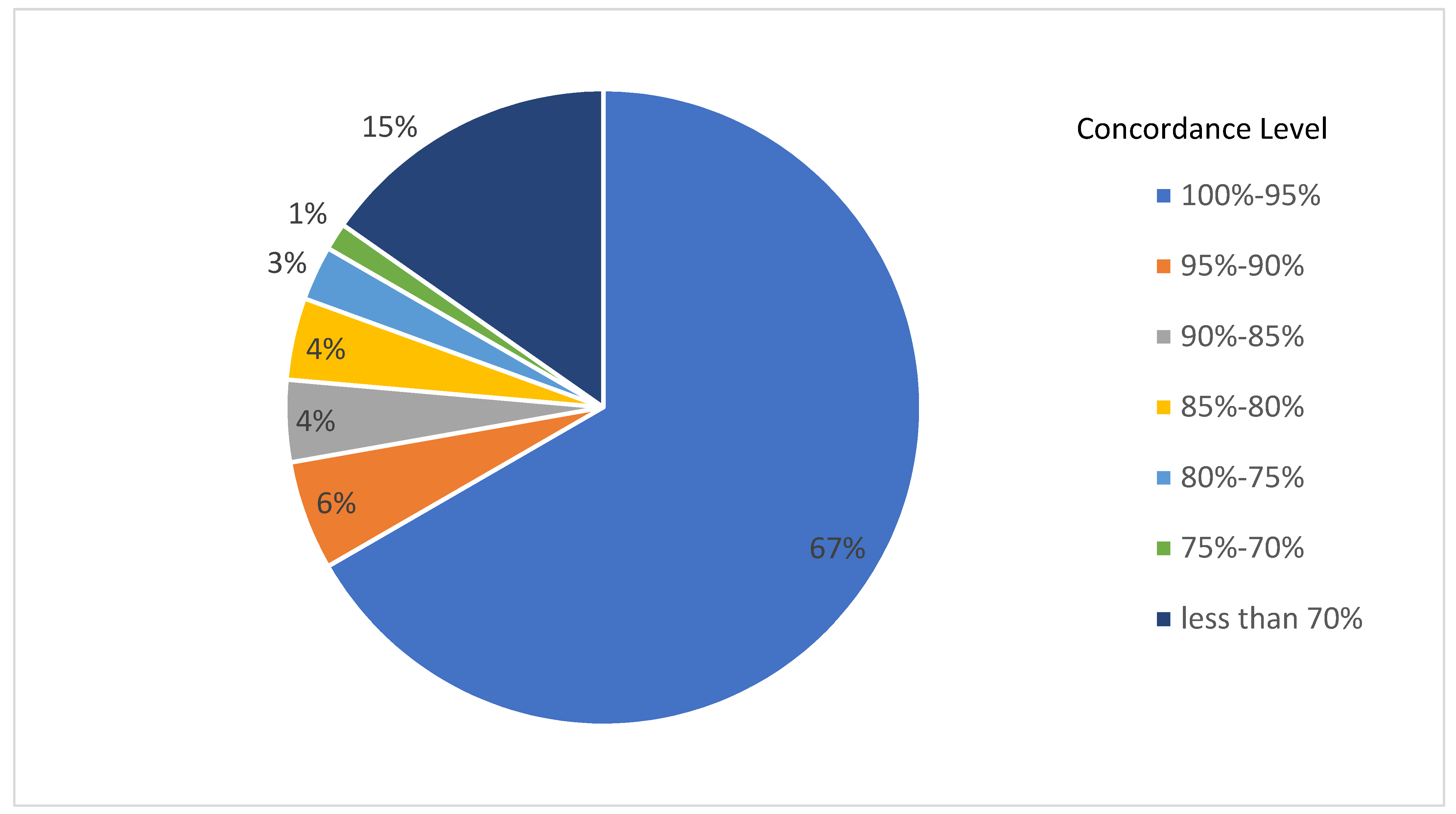
Since we established the superiority of the multivariate clustering over the univariate ones, we can analyze the concordance level between the dominant node and its neighbors.
In
Figure 2, we show the concordance level inside each one of the resulting mT-MDS neighborhoods. In 48 of the 72 neighborhoods, or 67% of the total, we have more than 95% concordance between the dominant node and its neighbors.
5. Discussion and Conclusions
In this paper, we presented an extension of an already proposed methodology of graph theory to optimize the supervision of complex banking networks. We introduce the multivariate Threshold–Minimum Dominating Set (mT-MDS), to identify a subset of banks with three distinct characteristics: (a) small in size, (b) representative enough for the whole network, and (c) able to act as a gauge of its respective neighborhoods. The proposed methodology outperforms the T-MDS method in terms of efficient classification of both solvent and failed banks. We attribute this superiority in terms of its ability to form multivariate networks exploiting information from different variables. Considering the latest consensus which supports the notion that the supervision of the whole banking system should be empowered to a single authority, we recommend the mT-MDS method as an auxiliary monitoring tool. The method’s efficiency is tested in a network of 570 American banks, 429 solvent banks, and 141 failed ones. The network is constructed in terms of two variables: the Tier 1 (core) risk-based capital over total assets, and the total interest expense over total interest income. We compare the performance of both methods (mT-MDS and T-MDS) in terms of efficiency and accuracy. The results indicate that the multivariate T-MDS method outperforms the respective univariate T-MDS method.
The empirical results show that the proposed methodology can be successfully employed by policy makers, banking sector regulators, and central banks. The use of this methodology as an auxiliary tool in the full arsenal of a regulator can improve the efficient supervision of a large banking network. This methodology has the advantage that provides fast results with minimal cost, and thus, it can be used as often as it is required by the supervisor. Moreover, we have seen above that it provides efficient and accurate information for the whole banking network while only monitoring the banks that are identified as core banks: the T-MDS nodes that effectively represent their whole neighborhood and the isolated ones.
In future work, we will consider a rolling window approach with a stable or varying temporal weight to introduce a dynamic feature and test the evolution of the banking network with respect to time.


