1. Introduction
It is well known now that the Black–Scholes model, which is a breakthrough in the financial area, is inadequate to describe asset returns and behaviors of the option markets (see
Dragulescu and Yakovenko 2002). This is because the Black-Scholes model assumes that the underlying asset satisfies the lognormal distribution, the right tail of which has quite often displayed a mismatch with empirically observed data. One possible remedy is to assume that the volatility of the asset price also follows a stochastic process (see
Ball and Roma 1994;
Fouque et al. 2000;
Heston 1993;
Hull and White 1987), rather than a constant, as assumed in the original Black–Scholes’ framework. In this paper, we use the stochastic model introduced by
Heston (
1993) to price American options. In this model, we assume that the variance (the square of the underlying price volatility) follows a random process known in the financial literature as the Cox–Ingersoll–Ross (CIR) process and in mathematical statistics as the Feller process (see
Feller 1951;
Fouque et al. 2000). Empirical studies suggest that this non-negative and mean-reverting process is indeed more consistent with the observations of real markets (see
Bakshi et al. 1997;
Pan 2002;
Tompkins 2001). For example,
Dragulescu and Yakovenko (
2002) showed that the time-dependent probability distribution of the changes of the stock index generated in the Heston model agrees well with the Dow Jones index after a careful calibration process to determine the appropriate parameters to be used in the model. Supported by much empirical evidence in the literature already, the Heston model has recently received much research attention in traditional finance, as well as quantitative finance, particularly in the latter (see
Altmayer and Neuenkirch 2016;
Malham et al. 2021;
Mickel and Neuenkirch 2021 and the references therein). In this paper, we shall complement the existing literature with a study on the asymptotic behavior of optimal exercise price near expiry of an American put option under a typical stochastic volatility model.
As is well known now, the main difficulty for pricing American options stems from the inherent nonlinear nature of the option contract itself, i.e., the additional right written in the contract for the holder to exercise the option at any time prior to the expiry date. In the context of partial differential equation (PDE) approaches, this is reflected in the fact that the corresponding PDE is associated with an unknown moving boundary, and the problem thus becomes a moving boundary problem. As a result, no useful analytical methods are hitherto available for pricing American options under the Heston model, and thus, numerical methods are preferred by market practitioners. However, it is usually difficult to retain accuracy in approximating the optimal exercise price by means of the numerical methods, and the inaccuracy becomes more intolerable when the time is closer to expiry. This is because within the short tenor, the velocity, with which the optimal exercise price reaches its final value, is extremely fast and is thus difficult to approximate by numerical methods. For example, when using the predictor–corrector finite difference scheme (see
Zhu and Chen 2011), a very fine discretization must be adopted near expiry, which is both expensive and limited in accuracy. Therefore, it is quite reasonable to infer that, under the Heston model, the optimal exercise price is also singular at expiry, which is true under the Black–Scholes’ framework (see
Evans et al. 2002). On the other hand, it is quite useful to determine the asymptotic behavior of the optimal exercise price near expiry, since this asymptotic solution can be used as a complement to the numerical approaches to calculate the option values and the optimal exercise price for other larger times away from the expiry.
In the literature, some analyses of the asymptotic behavior of the optimal exercise price near expiry have already been carried out. For instance,
Barles et al. (
1995) derived the first term for the optimal exercise price of American puts on a non-dividend-paying underlying by constructing a subsolution, as well as a supersolution. The examples in their paper considered options with maturities less than one year, in which case, the inaccuracy of the approximation was not significant.
Chen and Chadam (
2007) analyzed the same problem as Barles et al. did and provided four approximations for the optimal exercise prices of American puts with different maturities by the method of integral equations.
Evans et al. (
2002) considered the asymptotic behavior of the optimal exercise price near expiry on an asset with a constant dividend yield rate. The approximation was derived both with the utilization of the method of integral equations and the method of matched asymptotic expansions and was expected to be useful for time scales in the order of days and weeks from expiry. Moreover,
Chen and Zhu (
2009) extended Evans et al.’s results to the local volatility model, in which the volatility is assumed to be dependent on both time and the underlying asset price.
Yang (
2019) considered the short-maturity asymptotic behavior of the optimal exercise price of American lookback options under the random walks of the order-two model. On the other hand, it is a non-trivial task to derive asymptotic behaviors for multi-dimensional problems, and thus, this has received much research interest. For example,
Qin et al. (
2019) derived the asymptotic behavior of the optimal exercise strategy for a small number of executive stock options. It is also not easy, as will be shown in this paper, to determine the asymptotic behavior of the optimal exercise price near expiry under the Heston model, since in this case, the optimal exercise price depends, in addition to time, on the dynamics of volatility as well. In other words, the introduction of a second stochastic process has produced a number of new phenomena, which have in turn made the problem much more complicated and totally different from the case with a single stochastic process being used to describe the behavior of the underlying asset only while the volatility is assumed to be a constant.
The aim of this paper is to present an explicit analytical approximation for the optimal exercise price near expiry under the Heston model by means of the method of matched asymptotic expansions. The approximation could help readers understand clearly the near-expiry behavior of the optimal exercise price, which is indeed useful for both theoretical and practical purposes. It turns out that, even with stochastic volatility taken into consideration, the convergence rate for the calculation of the optimal exercise price is almost the same as that for the constant volatility case.
The paper is organized as follows. In
Section 2, we introduce the PDE system that the price of an American put option must satisfy under the Heston model. In
Section 3, we deduce the asymptotic behavior of the optimal exercise price near expiry by using the singular perturbation method. In
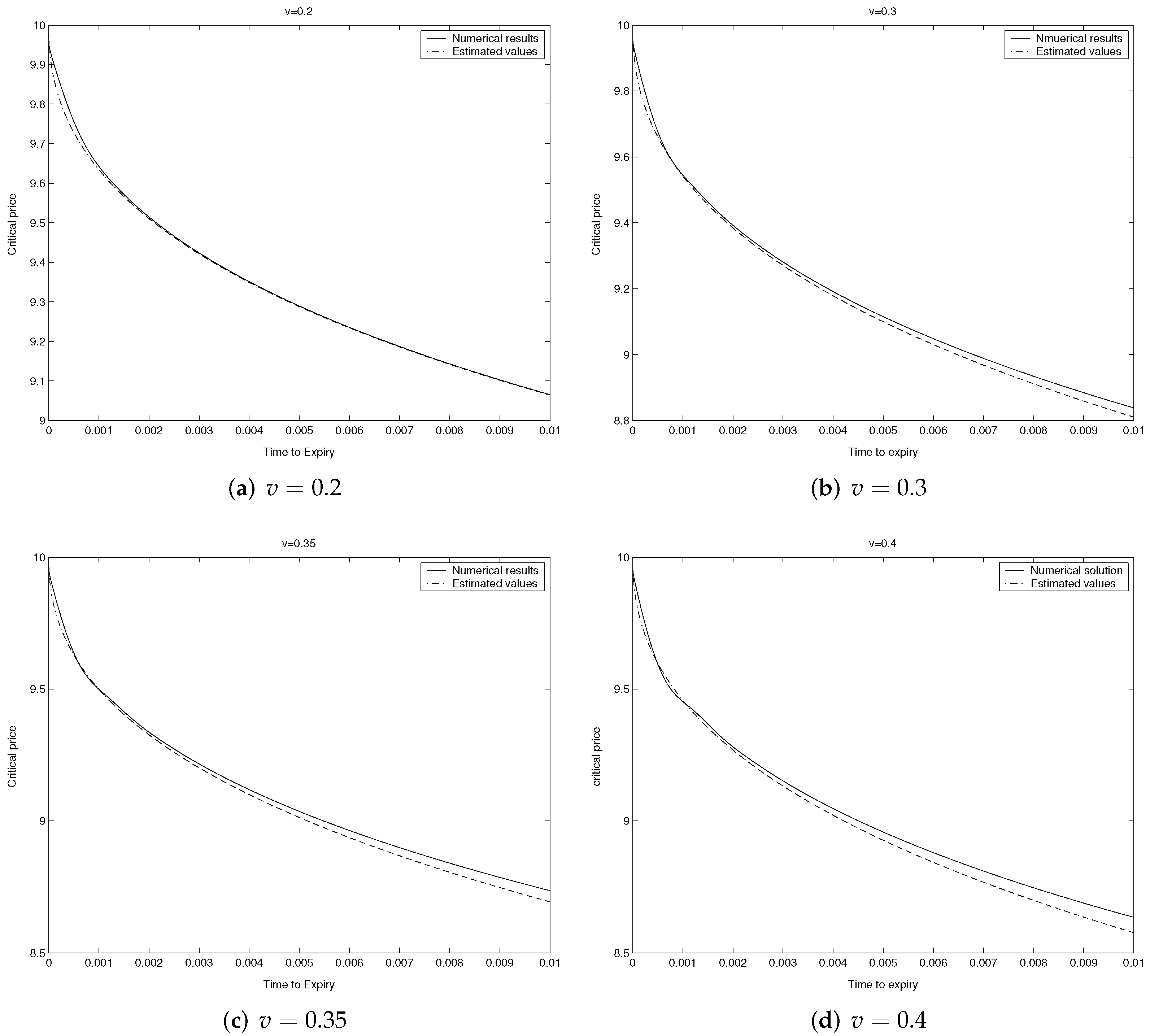
Section 4, we compare our approximation with the numerical results calculated by the predictor–corrector finite difference method (see
Zhu and Chen 2011), to illustrate the reliability of our asymptotic solution. Concluding remarks are given in
Section 5.
2. American Puts under the Heston Model
In this section, the Heston model and the PDE system for American puts underneath will be briefly reviewed. There are two main reasons why we choose the Heston model for the current work. Firstly, various studies (see
Bakshi et al. 1997;
Pan 2002;
Tompkins 2001) suggest that the Heston model is consistent with the real market. Secondly, this model is analytical achievable only for European options. In the case of American options, no analytical solution for American options under the Heston model has been discovered yet.
The hypotheses used in the current paper are the same as those of the Heston model. In the Heston model, the underlying
, as a function of time, is assumed to follow the stochastic differential equation (SDE) of a geometric Brownian motion (GBM) in the It
form:
where
is the drift rate,
is a standard Brownian motion, and
is the standard deviation of the stock returns
. Furthermore, the variance
(the square of the volatility) is assumed to be governed by the following mean-reverting SDE:
Here,
is the long-term mean of
,
is the rate of relaxation to this mean, and
is the volatility of volatility.
is also a standard Brownian motion, and it is related to
with a correlation factor
. (
2) known in the financial literature as the CIR process and in mathematical statistics as the Feller process (see
Feller 1951;
Fouque et al. 2000).
Let
denote the value of an American put option, with
S being the price of the underlying asset,
v being the variance, and
t being the time. Then, under the proposed processes (
1)–(
2), it is shown that the valuation of an American put option can be formulated as a free boundary problem (see
Zhu 2006), in which the boundary location itself is part of the solution of the problem. Specifically,
satisfies
This PDE system is defined on , and . We remark that in the above PDE system, K is the strike price, D is the dividend yield, is the expiry date, and r is the risk-free interest rate. Unlike the Black–Scholes’ case, the unknown optimal exercise price now depends on both the time and the volatility.
For simplicity, in our work, we assume that
r is greater than
D. A similar analysis can also be carried out for the case of
, and is thus not included in the current paper. It should be remarked that, when
, the riskless growing argument proposed in
Zhu and Chen (
2011) also holds, and thus, the boundary conditions established therein can still be used here. Moreover, it is also straightforward to show that (see
Zhu and Chen 2011):
which financially simply states that at the expiration date or when the spot volatility is zero, the optimal exercise price is equal to the strike price. However, just as a similar case of the Stephan problem (see
Zhu 2006), the “velocity”, with which the optimal exercise price reaches its final value, is extremely fast and is difficult to approximate by numerical approaches. Therefore, in the next section, we shall construct the asymptotic behavior of the optimal exercise price near expiry by using the method of matched asymptotic expansions.
3. Matched Asymptotic Expansions for the Optimal Exercise Price Near Expiry
To make the analysis convenient, we shall first non-dimensionalize all variables by using the new variables
where the parameters
q and
d are defined as
respectively. Then, (
3) can be written in the dimensionless form:
together with two more conditions for the optimal exercise price:
One should notice that, although the governing differential equation itself in (
4) is linear in terms of the unknown function
P, it is the unknown boundary that has made this PDE system highly nonlinear. The nonlinearity of the problem will be clearly manifested once a Landau transform is used to convert the moving boundary problem into a fixed boundary problem, as demonstrated by
Zhu and Chen (
2011). On the other hand, the high nonlinearity, as well as the introduction of another new variable
v has resulted in the analytical methods being less achievable than the Black–Scholes’ case (see
Evans et al. 2002). Consequently, we shall use the method of matched asymptotic expansions, which is an ideal tool to deal with the nonlinear problems, to construct an approximation of
for the PDE System (
4). Hereafter, we only consider the options with a short tenor, i.e.,
where
and
is a small positive parameter. By substituting (
6) into (
4), we obtain the PDE system for
:
Unlike the constant volatility case discussed in
Evans et al. (
2002), the PDE System (
7) needs to be dealt with with care; there are several different regions, or the so-called “boundary layers”, in which either the unknown function
P or its partial derivatives change rapidly. The increased complexity, as will be shown later, is a result of the introduction of stochastic volatility and, consequently, a new dimension of the PDE system. The “boundary layer” is a phrase commonly used in physics and fluid mechanics to describe the layer of fluid in the immediate vicinity of a boundary surface (see
Friedman 2008), and it has been adopted in most of singular perturbation analyses as well. Therefore, we shall also use it in this paper to derive the specific boundary layer structure for the PDE System (
7).
The procedure usually begins with the assumption that the solution can be expanded in powers of
, i.e.,
in which the subscript stands for the outer solution in the region outside of boundary layer where a singular expansion is required to deal with rapid changes of the value of
P or its derivatives. According to the fundamental theory of the method of matched asymptotic expansions
Smith (
2009), only a regular expansion in the form of (
8) is needed for the “outer region”; the correct order for the entire problem will be automatically determined once the “inner solution” and “outer solution” are forced to match. After some simple calculations, we obtain the solution as
It should be noted that the above solution is valid for the domain
,
, and fails to satisfy the boundary condition at
. Therefore, there is a boundary layer near
, with the layer thickness in the order of
. It can be inferred that, in order to satisfy the boundary condition at
, the exact solution of (
7), compared with
, changes rapidly only within the
neighborhood of
. On the other hand, in the traded market, the volatility value is usually very small, and the highest value of the volatility that has ever been recorded on the Chicago Board Options Exchange (CBOE) is only 0.85 (see
CBOE 2022). Therefore, with these two points in mind, it is perfectly justifiable to not analyze this boundary layer at all; our solution will be a reasonably good approximation for any large enough, but finite
v values.
On the other hand, it is clear that as
, too many terms on the right-hand side of the governing equation contained in (
7) have been dropped, and thus, we need to perform an asymptotic analysis in the vicinity of
. By using the stretched variable:
and substituting (
10) into (
7), we obtain
The significant degeneration of the above operator arises if
, and thus, the boundary layer near
is with the thickness of
. Assuming that
has a regular expansion in this region, we write
where the explicit analytical expressions of
,
, and
are derived in
Appendix A. The solution derived in this boundary layer can be referred as the inner solution with respect to (with respect to hereafter)
.
It can be easily shown that the first-order derivative of
with respect to
v becomes unbounded at the corner
. Consequently, the derivatives of
with respect to
v cannot be ignored when deriving the PDE system for
around that corner. Another local analysis is again needed. By setting
and investigating the significant degeneration of the corresponding operator, it is obvious that
is a well-balanced choice. Assuming that
(the solution at the corner) can be expanded in powers of
, we obtain
where the explicit analytical expressions of
,
, and
are derived in
Appendix B. Furthermore, it can be easily shown that
is continuous, but not differentiable with respect to
X at the corner
. Thus, the following stretched variables are needed:
where
are determined by investigating the significant degeneration of the corresponding operator again.
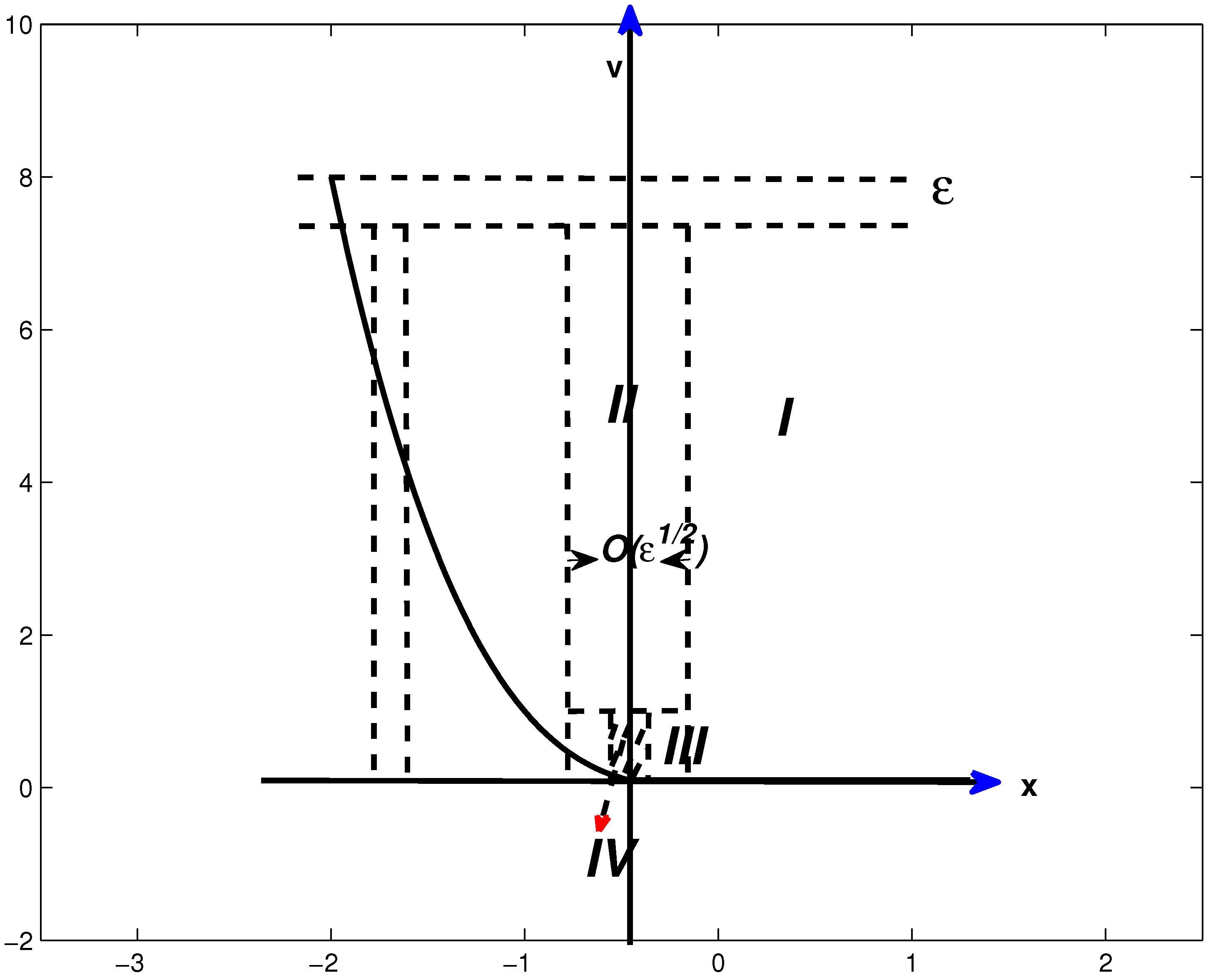
The above analysis has clearly demonstrated the boundary layer structure of our problem, as shown in
Figure 1, where the Roman numbers
I,
,
, and
stand for four different regions in which local analysis needs to be carried out consecutively. In particular, Region
I represents the valid domain of
, while Region
shows the
boundary layer near
. Regions
and
denote the corner boundary layers, and they are defined as
respectively. Moreover, near
, there might be another boundary layer, which will be discussed later. Note again that the
boundary layer near
has been ignored.
It should be remarked here that the introduction of a second stochastic process for
v has indeed made the analysis much more complicated and totally different from that of the Black–Scholes’ case, as shown in
Evans et al. (
2002). The complexity, as well as the difference has been clearly manifested when analyzing the solution within the domain
,
. Here, the notation
denotes the neighborhood of a point
a with radius
, i.e.,
In the classical Black–Scholes’ case, the analysis usually stops once the inner solution within the
boundary layer near
has been found. Under the Heston model, however, the “inner” region
(relative to the “outer” Region
needs to be further divided into another set of “inner” and “outer” regions because there exists another boundary layer in the
v direction as a result of Region
still containing the singular point at the origin. This new inner region is denoted as Region
. Similarly, the same process needs to be repeated, which yields Region
(the dashed area of
Figure 1) as a boundary layer in
x again. It is envisaged that this “cascade” phenomenon of sub-dividing regions is a particular feature associated with the Heston model when it is used to price American options. However, since we are only interested in an approximate solution, based on the method of matched asymptotic expansions, of
, it suffices to stop the sub-division at Region
, as shall be discussed later.
With the division of the original solution domain into the above four regions, we can now prove the following lemma for the asymptotic behavior when . Note that hereafter, we shall use a new definition , i.e., , if , and for . As shall be demonstrated, this new definition enables us to give a sharp estimate of the target functions.
Lemma 1.
(i) For , we have . (ii) For , where , we have , and the leading-order term of , say , should be bounded as and satisfy , where .
Proof.
(i) The first part of the lemma is proven by means of the method of proof by contradiction. Assuming that
, we have
, where
should have finite values for any
and
. Therefore, we can rescale
and expand it in terms of
, i.e.,
In order to satisfy the moving boundary conditions, the leading-order term should at least satisfy
which yields
However, when
, the only solution of (
12) and (
13) is
, and this is in contrast with our assumption that
. Therefore, when
, the location of the free boundary should be outside the
layer near
, and thus,
. This completes the proof.
(ii) It is straightforward to show that if
, (
12) and (
13) are always satisfied. On the other hand, when
, the leading-order term of
, i.e.,
, can be bounded and satisfy
at the same time. Therefore, when
, where
,
should be located inside
. This completes the proof. □
Since the location of the free boundary differs with respect to v, it is much more convenient to discuss the asymptotic behavior of in different ranges of v separately.
Case I.
In this case,
is located outside
, which indicates that there is another boundary layer near
. Now, we perform the local analysis in the vicinity of
by using the stretched variable:
where
. Substituting (
14) into the governing equation contained in (
7), we obtain
Again, an expansion in regular powers of
gives the solution of (
15) as
In order to match the solution in Region
with the solution near
, we found the asymptotic behaviors of
,
, and
as
:
where
.
Now, if we follow
Evans et al. (
2002) and match the
values of (
11) and (
16) by taking the limit
, we obtain the following transcendental equations:
which lead to the solutions of the form
respectively, after higher-order terms are ignored.
It should be remarked that matching
values is not the unique choice.
Evans et al. (
2002) did it in this way without any detailed explanation. In fact, this approach may be at odds with the conventional method of matched asymptotic expansions in which
P, instead of
, values should be matched in the “inner” and “outer” regions. Clearly, if a solution is obtained with
P values being matched, so should the
values, provided that the
P function is of sufficient smoothness. However, the converse is not true. One naturally wonders whether or not the two different approaches would lead to the same conclusion, once all the higher-order terms are ignored. Without a great deal of additional effort, it can be shown that matching the
P values of (
11) and (
16) by taking the limit
leads to
In comparison with (
17) and (
18), it is much more difficult to go through some additional order analysis to simplify (
21), in order to analytically obtain the asymptotic behavior of
like those presented in (
19) and (
20). However, it can still be shown that
lies between
and
(see Lemma 2 below), where
is solved from matching with
. Hence, as
approaches zero, the difference between
and
will become smaller. It should be noted that we only need to consider the negative root of (
21) because of the physical restriction that
.
Lemma 2.
For small τ, (21) has only one negative solution , and moreover, it satisfieswhere Proof. Comparing (
24) with (
21), it is obvious that
. Then, taking the first-order derivative of
with respect to
x, we obtain:
Since the parameters a, , and d are all greater than zero, we have for any . Therefore, is monotonically increasing for negative x values.
On the other hand, it is straightforward to show that when
,
Furthermore, for reasonably small
, we have
Therefore,
and
. Based on the monotonicity of
, the only negative root of
f should lie between
and
. Similarly, we can show that when
, it lies between
and
. Therefore, for small
, (
21) has only one negative solution
, and moreover, it satisfies
This completes the proof. □
On the other hand, Equation (
21) can also be numerically solved, and numerical evidence indeed suggests that the difference between
and
is negligible. This probably explains why
Evans et al. (
2002) chose to match the
values in their analysis.
By substituting (
19)–(
20) into (
11), we find that the free boundary conditions can be satisfied in the following asymptotic sense, i.e.,
where
stands for the exact free boundary.
Case II.
According to the second part of Lemma 1,
should be located inside
. Now, we assume that (
11) can satisfy the conditions across the free boundary. By taking the limit
, we deduce the asymptotic behavior of
,
and
, respectively, as:
where
. It is not strange that the asymptotic behaviors of
,
, and
as
are quite similar to those derived in Case I, since when taking the limit
, it is equivalent to
, which is also equal to
and
.
On the other hand, upon applying the free boundary conditions on (
11), the leading-order term of
should at least satisfy
which is the same as what we have obtained in Case I. It is now quite trivial to show that the leading-order term of
is the same as the one derived in Case I, and the expansion satisfies the free boundary conditions in almost the same asymptotic sense, i.e.,
Case III.
In this case, if we follow the procedure described previously, we should first determine whether
or not, which is equivalent to analyzing whether the solution in Region
can satisfy the free boundary conditions or not. It is straightforward to show that the governing equation for the solution in Region
is
which contains all the derivatives the original equation has. Now, we are in an unfortunate situation of having to solve almost the full problem to be able to determine what is going on in Region
. If we could solve this problem, one might wonder why it was necessary to bother with an approximation in the first place. There is no need to argue with this sentiment, and this is indeed one of the situations where the perturbation methods show some of their limitations. However, there are several remarks that should be made. Firstly, though this layer problem cannot be solved in a closed form, we may still be able to extract some useful information about the solution. Secondly, this problem can be further dealt with if we again apply the method of matched asymptotic expansions to this corner, i.e., by rescaling
, and following almost the same procedure as demonstrated previously. Fortunately, there is no need to go through such a cumbersome analysis again. In order to demonstrate the reasons in a clear way, we adopt a new notation
for the actual optimal exercise boundary in this case.
As it turns out, when
, the location of the optimal exercise boundary should be located either inside
or outside. However, it is claimed that no matter what is the truth, the approximation of
derived before for
can still be used here. Firstly, if
is located outside
, then (
33) is defined on
Taking the corresponding boundary conditions into consideration, it can be identified that
, with
twice continuously differentiable with respect to
or
V on
. The stretched
, which is derived in the previous two cases, reads
which means that
is finite for any
and
. Based on the continuous property of both
and its first-order derivative with respect to
, it is clear that if we adopt the approximation of
derived previously as the free boundary here, then the option price
satisfies the free boundary conditions in the
sense, which is almost the same as the previous two cases; see (
27) and (
28) and (
31) and (
32).
Secondly, if is located inside , it is meaningless to derive its actual form, since is already a good approximation for .
Based on Case I to Case III, it can be concluded that when
, (
19) can be used as an approximation for small
and
. Written in original variables, we obtain the leading-order term of the optimal exercise price as:
For
, (
20) is valid for small
and
. Therefore,
It is quite interesting to note that the leading-order terms of the optimal exercise price are similar to the ones with constant volatility (see
Evans et al. 2002), with
being substituted by
v. One possible reason is that the moving boundary only occurs along the
S direction, and no critical points appear along the
v direction. Furthermore, in Case I and Case II, the impact of
v is less significant, so that
v becomes a parameter rather than a variable; (see (
A1)–(
A3)). However, the option prices are much more complicated and totally different than those with constant volatility; (see (
A5), (
A11), and (
A15)).


