
Copulas and Portfolios in the Electric Vehicle Sector


Abstract
:1. Introduction
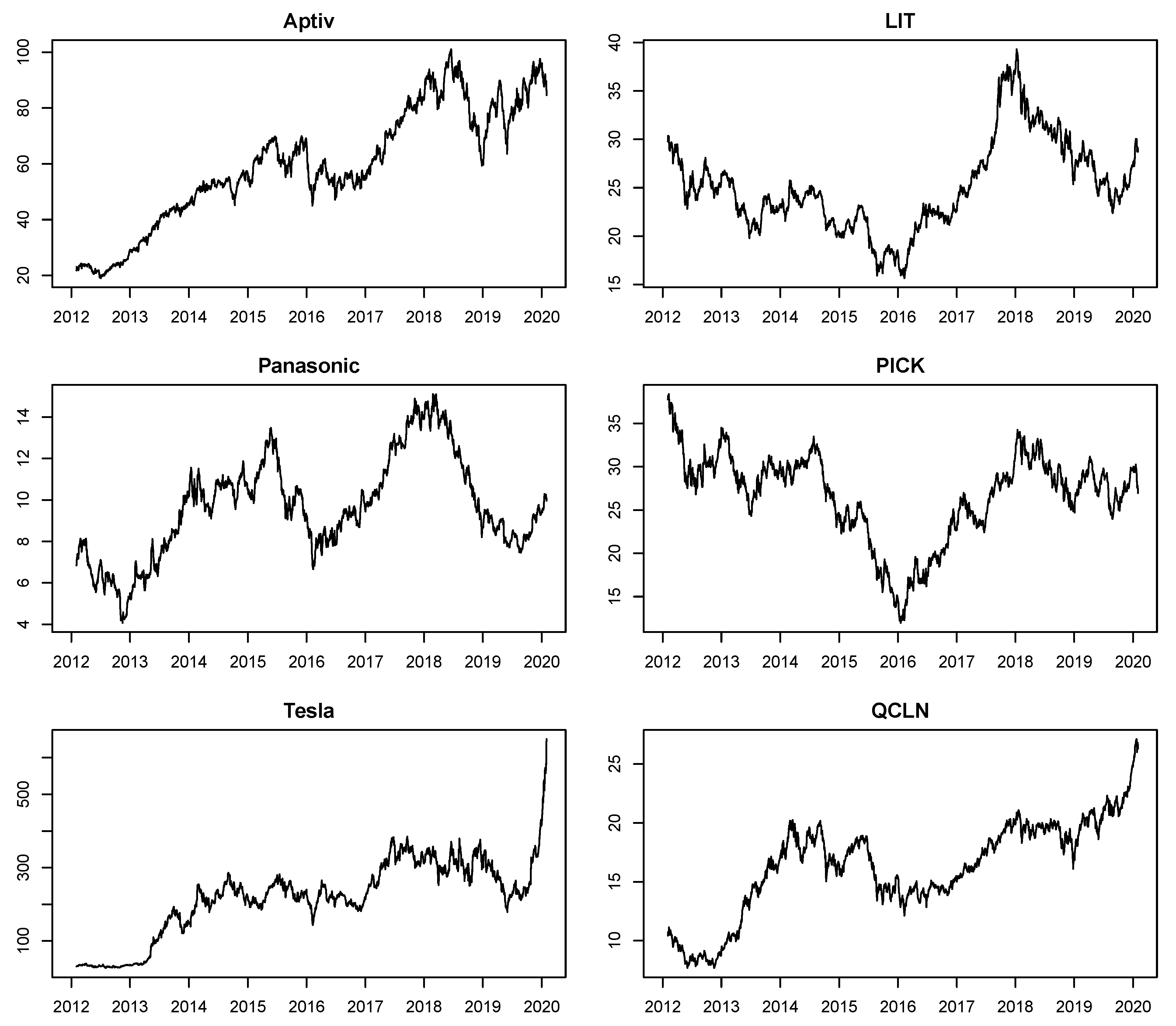
2. Data
3. Theoretical Framework and Methods
3.1. Marginal Models
3.2. Copula Models
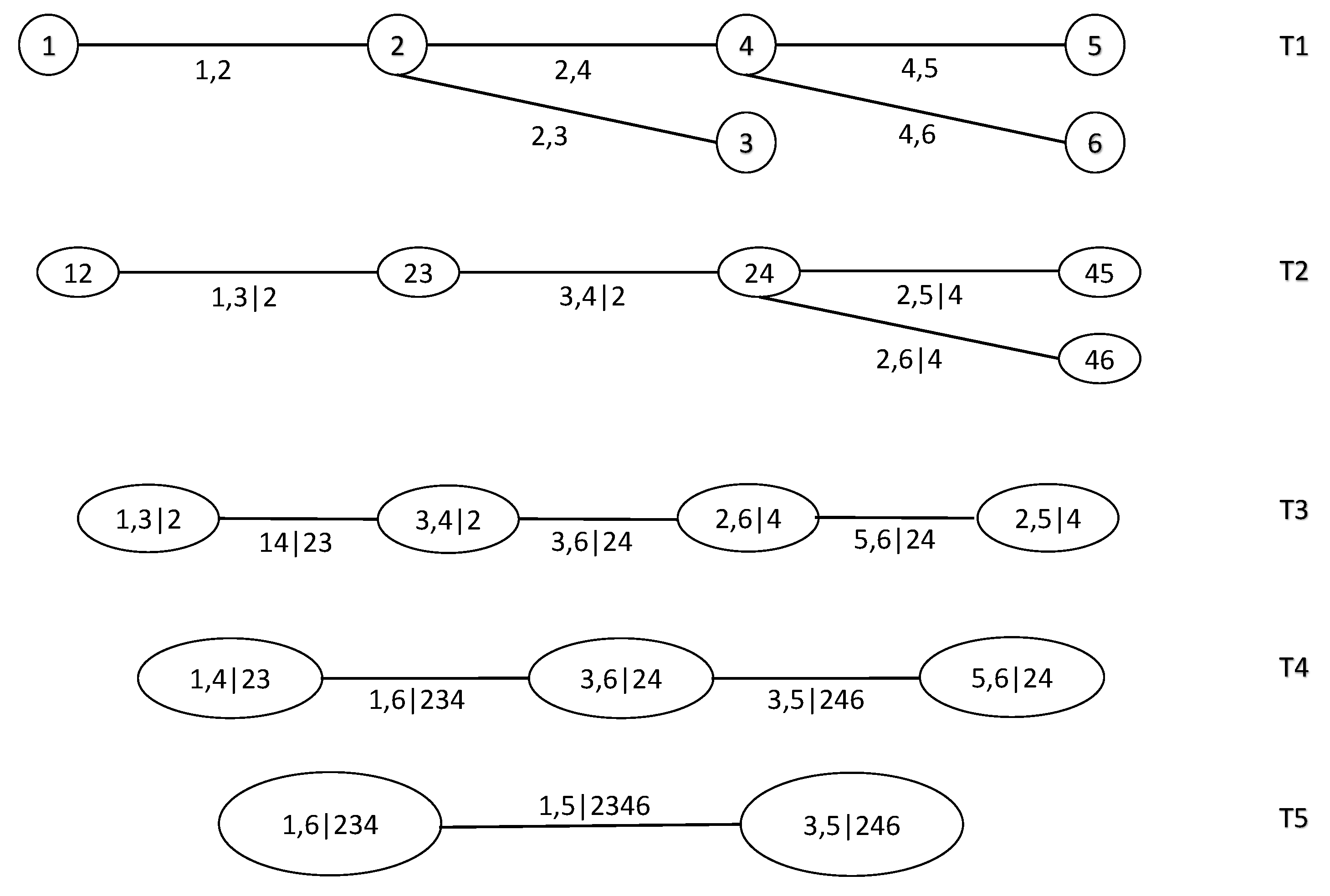
3.2.1. Vine Copulas
3.2.2. Model Building and Selection with Vine Copulas
3.3. Joint Models
3.4. Rolling-Window Portfolio Optimization with Expected Shortfall
- Target expected return: ;
- No short sales: ;
- Normalization of weights: .
- For each asset, estimate a marginal model of its returns;
- Estimate a copula model and obtain a one-day-ahead density forecast of the multivariate joint distribution of the asset returns;
- Simulate a large sample of multivariate returns from the forecast density;
- Apply numerical optimization of the given criterion (i.e., minimize ES for a given expected value) on the simulated returns from step 3 to obtain optimal portfolio weights;
- Multiply the simulated returns from step 3 by the weights from step 4 to obtain simulated portfolio returns.
- Estimate the portfolio VaR and ES nonparametrically: (i) where is the empirical quantile defined in Hyndman and Fan (1996) and used as the default option in the quantile function in R; (ii) where are the simulated portfolio returns and is the number of them satisfying the condition .
3.5. Performance Evaluation
3.5.1. Statistical Adequacy
3.5.2. Financial Performance
4. Empirical Results
4.1. Marginal Models
4.2. Copula-Based Portfolios
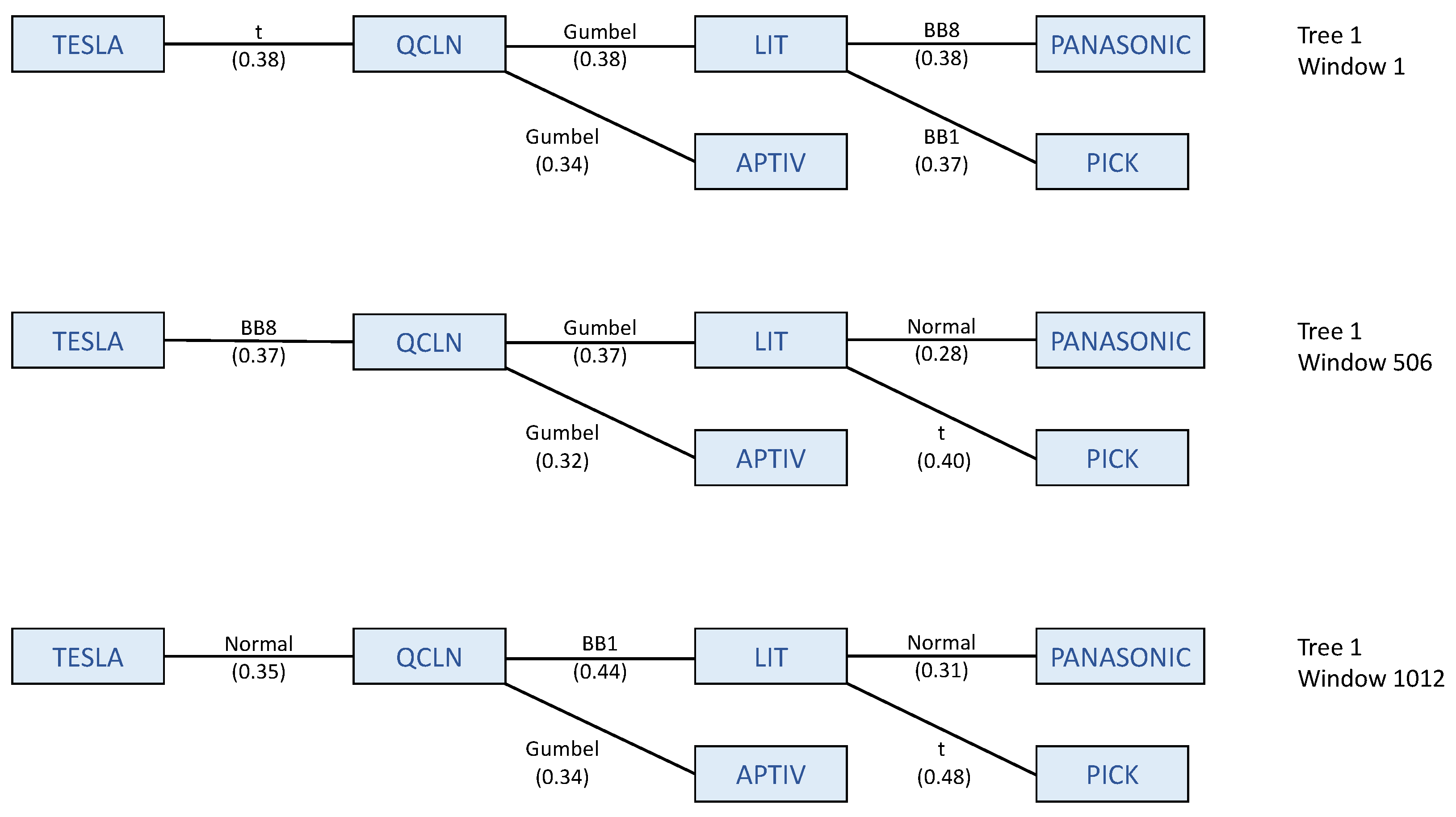
4.2.1. R-Vine Structure
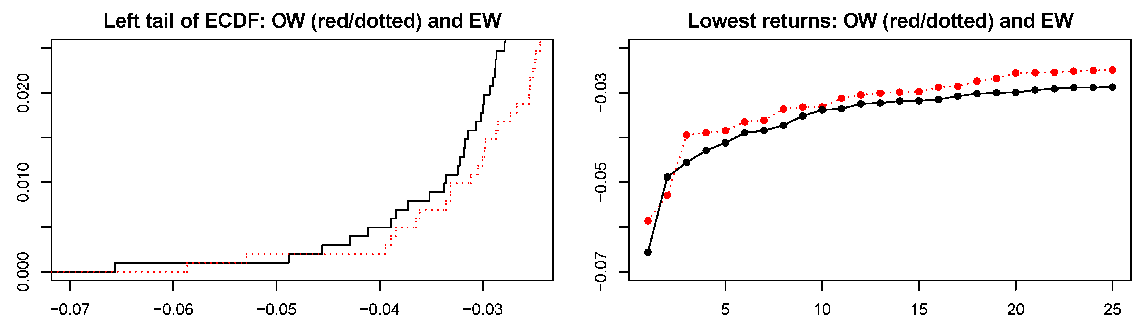
4.2.2. Optimally vs. Equally Weighted Portfolios
4.3. Financial Assessment of Portfolios
5. Conclusions
Author Contributions
Funding
Data Availability Statement
Conflicts of Interest
Appendix A. Exchange Traded Funds

| Holding | Ticker | Weighting |
|---|---|---|
| BHP Billiton Ltd | BHP:AUX | 10.84% |
| Rio Tinto PLC | RIO:LSE | 8.78% |
| Vale SA | VALE3:SAO | 5.44% |
| Glencore PLC | GLEN:LSE | 4.66% |
| Anglo American PLC | AAL:LSE | 4.00% |
| GMK Noril’skiy Nikel’ PAO | GMKN:MCX | 3.22% |
| Freeport-McMoRan Inc | FCX | 2.51% |
| Nucor Corp | NUE | 2.09% |
| Posco | 005490:KSC | 2.03% |
| ArcelorMittal SA | MT:AEX | 1.59% |
| Holding | Ticker | Weighting |
|---|---|---|
| Albemarle Corp | ALB | 19.78% |
| Sociedad Quimica y Minera de Chile SA | SQM | 12.74% |
| Tesla Inc | TSLA | 12.53% |
| Livent Corp | LTHM | 5.86% |
| Samsung SDI Co Ltd | 006400:KSC | 5.41% |
| LG Chem Ltd | 051910:KSC | 4.73% |
| Panasonic Corp | 6752:TYO | 4.56% |
| Byd Co Ltd | 1211:HKG | 4.51% |
| Simplo Technology Co Ltd | 6121:TWO | 4.16% |
| EnerSys | ENS | 4.09% |
| Holding | Ticker | Weighting |
|---|---|---|
| Tesla Inc | TSLA | 16.54% |
| Brookfield Renewable Partners LP | BEP.UN | 5.97% |
| Albemarle Corp | ALB | 5.53% |
| ON Semiconductor Corp | ON | 5.01% |
| Universal Display Corp | OLED | 4.92% |
| Enphase Energy Inc | ENPH | 4.24% |
| Solaredge Technologies Inc | SEDG | 3.76% |
| Cree Inc | CREE | 3.14% |
| First Solar Inc | FSLR | 3.09% |
| TerraForm Power Inc | TERP | 2.93% |
Appendix B. Traditional Copulas
Appendix B.1. Elliptical Copulas
Appendix B.2. Gaussian Copula
Appendix B.3. Student-t Copula
Appendix B.4. Archimedean Copulas
Appendix B.5. Clayton Copula
Appendix B.6. Frank Copula
Appendix B.7. Gumbel Copula
Appendix B.8. Joe Copula
| 1 | For more details on PICK, LIT and QCLN, see Table A1, Table A2 and Table A3, respectively, in Appendix A. |
| 2 | Orthants are a multivariate generalization of the bivariate quadrants. |
| 3 | None of the alternative, unreported model specifications that have been tried delivered more satisfactory results for these cases, leaving GARCH(1,1)-JSU as our top choice. |
| 4 | To minimize transaction costs, a private investor would normally prefer weights that do not vary substantially over time and do not require daily rebalancing of the portfolio. However, institutional investors acting on behalf of a large number of clients receive capital inflows daily and need to make new investments every day. Whenever a new investment is to be made (a new portfolio formed), it may be natural to look for a portfolio that has been estimated to be optimal for that day. This does not mean that the already existing portfolios would or should be rebalanced as frequently. |
| 5 | A null hypothesis that the expected annual returns on the two portfolios are equal cannot be rejected at any reasonable significance level, as a two-sided (one-sided) paired t-test yields a p-value of 0.58 (0.29). |
References
- Aas, Kjersti, Claudia Czado, Arnoldo Frigessi, and Henrik Bakken. 2009. Pair-copula constructions of multiple dependence. Insurance: Mathematics and Economics 44: 182–98. [Google Scholar] [CrossRef] [Green Version]
- Akaike, Hirotogu. 1973. Information theory and an extension of the maximum likelihood principle. In 2nd International Symposium on Information Theory. Budapest: Publishing House of the Hungarian Academy of Sciences, pp. 268–81. [Google Scholar]
- Basel Committee. 2016. Minimum capital requirements for market risk. In Technical Report, Bank for International Settlements. Basel: Basel Committee. [Google Scholar]
- Basel Committee. 2017. Pillar 3 disclosure requirements–consolidated and enhanced framework. In Technical Report, Basel Committee on Banking Supervision. Basel: Basel Committee. [Google Scholar]
- Bayer, Sebastian, and Timo Dimitriadis. 2020. Regression-based expected shortfall backtesting. Journal of Financial Econometrics. nbaa013. [Google Scholar] [CrossRef]
- BBC News. 2021. Elon Musk Becomes World’s Richest Person as Wealth Tops $185bn. BBC. Available online: https://www.bbc.com/news/technology-55578403 (accessed on 7 January 2021).
- Bedford, Tim, and Roger M. Cooke. 2001. Probability density decomposition for conditionally dependent random variables modeled by vines. Annals of Mathematics and Artificial Intelligence 32: 245–68. [Google Scholar] [CrossRef]
- Bedford, Tim, and Roger M. Cooke. 2002. Vines: A new graphical model for dependent random variables. The Annals of Statistics 30: 1031–68. [Google Scholar] [CrossRef]
- Bollerslev, Tim. 1986. Generalized autoregressive conditional heteroskedasticity. Journal of Econometrics 31: 307–27. [Google Scholar] [CrossRef] [Green Version]
- Breymann, Wolfgang, Alexandra Dias, and Paul Embrechts. 2003. Dependence structures for multivariate high-frequency data in finance. Quantitative Finance 3: 1–14. [Google Scholar] [CrossRef]
- Cherubini, Umberto, Elisa Luciano, and Walter Vecchiato. 2004. Copula Methods in Finance. Hoboken: John Wiley & Sons. [Google Scholar]
- Christoffersen, Peter F. 1998. Evaluating interval forecasts. International Economic Review 39: 841–62. [Google Scholar] [CrossRef]
- Christoffersen, Peter F., and Denis Pelletier. 2004. Backtesting value-at-risk: A duration-based approach. Journal of Financial Econometrics 2: 84–108. [Google Scholar] [CrossRef]
- Cont, Rama. 2001. Empirical properties of asset returns: Stylized facts and statistical issues. Quantitative Finance 1: 223–36. [Google Scholar] [CrossRef]
- Czado, Claudia. 2019. Analyzing Dependent Data with Vine Copulas. Berlin/Heidelberg: Springer. [Google Scholar]
- Diebold, Francis X., Todd A. Gunther, and Anthony Tay. 1998. Evaluating density forecasts with applications to financial risk management. International Economic Review 39: 863–83. [Google Scholar] [CrossRef] [Green Version]
- Dissmann, Jeffrey, Eike C. Brechmann, Claudia Czado, and Dorota Kurowicka. 2013. Selecting and estimating regular vine copulae and application to financial returns. Computational Statistics & Data Analysis 59: 52–69. [Google Scholar]
- Engle, Robert F. 1982. Autoregressive conditional heteroscedasticity with estimates of the variance of United Kingdom inflation. Econometrica 50: 987–1007. [Google Scholar] [CrossRef]
- Forbes. 2020. Tesla Is Now the Worlds Most Valuable Car Company with a Valuation of 208 Billion. Forbes. Available online: https://www.forbes.com/sites/sergeiklebnikov/2020/07/01/tesla-is-now-the-worlds-most-valuable-car-company-with-a-valuation-of-208-billion/ (accessed on 3 March 2022).
- FT. 2020. Tesla Overtakes Toyota to Become World’s Most Valuable Carmaker. Financial Times. Available online: https://www.ft.com/content/1fd51f91-ff3c-4723-995c-f75f6629c66e (accessed on 1 July 2020).
- Hertzke, Patrick, Nicolai Muller, Patrick Schaufuss, Stephanie Schenk, and Ting Wu. 2019. Expanding Electric-Vehicle Adoption Despite Early Growing Pains. Boston: McKinsey & Company. [Google Scholar]
- Hyndman, Rob J., and Yanan Fan. 1996. Sample quantiles in statistical packages. The American Statistician 50: 361–5. [Google Scholar]
- IEA. 2020. Global Electric Car Sales by Key Markets, 2010–2020. Paris: IEA. [Google Scholar]
- Jarque, Carlos M., and Anil K. Bera. 1980. Efficient tests for normality, homoscedasticity and serial independence of regression residuals. Economics Letters 6: 255–9. [Google Scholar] [CrossRef]
- Joe, Harry. 1996. Families of m-variate distributions with given margins and m(m-1)/2 bivariate dependence parameters. In Lecture Notes-Monograph Series. Hayward: Institute of Mathematical Statistics, pp. 120–41. [Google Scholar]
- Joe, Harry. 1997. Multivariate Models and Multivariate Dependence Concepts. Boca Raton: CRC Press. [Google Scholar]
- Joe, Harry, and James Jianmeng Xu. 1996. The Estimation Method of Inference Functions for Margins for Multivariate Models. Vancouver: UBC Faculty Research and Publications. [Google Scholar] [CrossRef]
- Johnson, Norman L. 1949. Systems of frequency curves generated by methods of translation. Biometrika 36: 149–76. [Google Scholar] [CrossRef] [PubMed]
- Kendall, Maurice G. 1938. A new measure of rank correlation. Biometrika 30: 81–93. [Google Scholar] [CrossRef]
- Kupiec, Paul. 1995. Techniques for verifying the accuracy of risk measurement models. The Journal of Derivatives 3: 73–84. [Google Scholar] [CrossRef]
- Kurowicka, Dorota, and Roger M. Cooke. 2006. Uncertainty Analysis with High Dimensional Dependence Modelling. Hoboken: John Wiley & Sons. [Google Scholar]
- Markowitz, Harry. 1952. The utility of wealth. Journal of Political Economy 60: 151–58. [Google Scholar] [CrossRef]
- McNeil, Alexander J., and Rüdiger Frey. 2000. Estimation of tail-related risk measures for heteroscedastic financial time series: An extreme value approach. Journal of Empirical Finance 7: 271–300. [Google Scholar] [CrossRef]
- Nagler, Thomas, and Thibault Vatter. 2019. rvinecopulib: High Performance Algorithms for Vine Copula Modeling, R Package Version 0.5.1.1.0.
- Nelsen, Roger B. 2006. An Introduction to Copulas. Berlin/Heidelberg: Springer. [Google Scholar]
- Patton, Andrew J. 2006. Modelling asymmetric exchange rate dependence. International Economic Review 47: 527–56. [Google Scholar] [CrossRef]
- R Core Team. 2020. R: A Language and Environment for Statistical Computing. Vienna: R Foundation for Statistical Computing. [Google Scholar]
- Rodriguez, Juan Carlos. 2007. Measuring financial contagion: A copula approach. Journal of Empirical Finance 14: 401–23. [Google Scholar] [CrossRef] [Green Version]
- Sklar, Abe. 1959. Fonctions de riépartition á n dimensions et leurs marges. Publications de l’Institut Statistique de l’Universite de Paris 8: 229–31. [Google Scholar]
- Statista. 2021a. Best-Selling Plug-in Electric Vehicle Models Worldwide in 2020. Hamburg: Statista. [Google Scholar]
- Statista. 2021b. Estimated Plug-in Electric Vehicle Sales Worldwide in 2020, by Automaker. Hamburg: Statista. [Google Scholar]
- Woodward, Michael, Jamie Hamilton, and Bryn Walton. 2020. Battery Electric Vehicles: New Markets, New Entrants, New Challenges. Deloitte. Available online: https://www2.deloitte.com/uk/en/insights/industry/automotive/battery-electric-vehicles.html (accessed on 20 February 2021).
- Yollin, Guy. 2009. R tools for portfolio optimization. In R/Finance Conference. Bellevue: Quantitative Research Analyst, Rotella Capital Management, vol. 2009. [Google Scholar]


| Aptiv | Panasonic | Tesla | LIT | PICK | QCLN | |
|---|---|---|---|---|---|---|
| Mean | 0.064 | 0.016 | 0.158 | −0.001 | −0.022 | 0.047 |
| Std. dev. | 1.746 | 1.847 | 3.181 | 1.363 | 1.624 | 1.460 |
| Min | −13.032 | −10.137 | −18.845 | −6.908 | −9.015 | −5.959 |
| Max | 10.356 | 11.520 | 21.829 | 8.260 | 6.544 | 6.239 |
| Skewness | 0.283 | 0.083 | 0.264 | −0.146 | −0.147 | −0.288 |
| Excess kurtosis | 3.569 | 3.080 | 5.705 | 2.146 | 1.596 | 0.919 |
| Jarque-Bera | 1109.5 *** | 808.44 *** | 2787.6 *** | 399.14 *** | 224.29 *** | 100.37 *** |
| ARCH-LM(15) | 42.129 *** | 118.69 *** | 132.14 *** | 156.79 *** | 141.95 *** | 151.00 *** |
| Normal | Aptiv | Panasonic | Tesla | LIT | PICK | QCLN |
|---|---|---|---|---|---|---|
| KS | 0.006 | 0.002 | 0.000 | 0.004 | 0.003 | 0.003 |
| VaR unc. | 0.010 | 0.884 | 0.355 | 0.193 | 0.265 | 0.137 |
| VaR cond. | 0.008 | 0.390 | 0.120 | 0.428 | 0.208 | 0.235 |
| VaR dur. | 0.699 | 0.672 | 0.683 | 0.772 | 0.898 | 0.829 |
| ES unb. | 0.026 | 0.020 | 0.000 | 0.029 | 0.090 | 0.009 |
| S-ESR | 0.234 | 0.218 | 0.052 | 0.006 | 0.353 | 0.011 |
| A-ESR | 0.234 | 0.197 | 0.055 | 0.006 | 0.341 | 0.020 |
| I-ESR-1s | 0.050 | 0.023 | 0.008 | 0.002 | 0.053 | 0.006 |
| I-ESR-2s | 0.101 | 0.047 | 0.017 | 0.004 | 0.105 | 0.012 |
| Johnson’s SU | Aptiv | Panasonic | Tesla | LIT | PICK | QCLN |
| KS | 0.174 | 0.194 | 0.417 | 0.315 | 0.142 | 0.704 |
| VaR unc. | 0.193 | 0.642 | 0.956 | 0.270 | 0.642 | 0.500 |
| VaR cond. | 0.150 | 0.749 | 0.074 | 0.387 | 0.525 | 0.488 |
| VaR dur. | 0.263 | 0.703 | 0.609 | 0.895 | 0.692 | 0.211 |
| ES unb. | 0.900 | 0.194 | 0.100 | 0.171 | 0.398 | 0.544 |
| S-ESR | 0.648 | 0.307 | 0.045 | 0.336 | 0.677 | 0.000 |
| A-ESR | 0.650 | 0.343 | 0.044 | 0.347 | 0.645 | 0.001 |
| I-ESR-1s | 0.535 | 0.473 | 0.581 | 0.206 | 0.346 | 0.717 |
| I-ESR-2s | 0.931 | 0.946 | 0.838 | 0.413 | 0.692 | 0.565 |
| Normal–Normal | Student–Johnson’s SU | Vine–Johnson’s SU | |
|---|---|---|---|
| Panel A: EW | |||
| KS | 0.043 | 0.111 | 0.441 |
| VaR unc. | 0.027 | 0.193 | 0.589 |
| VaR cond. | 0.075 | 0.286 | 0.838 |
| VaR dur. | 0.351 | 0.313 | 0.466 |
| ES unb. | 0.007 | 0.629 | 0.733 |
| S-ESR | 0.017 | 0.767 | 0.985 |
| A-ESR | 0.016 | 0.774 | 0.969 |
| I-ESR-1s | 0.002 | 0.237 | 0.499 |
| I-ESR-2s | 0.004 | 0.474 | 0.999 |
| Panel B: OW | |||
| KS | 0.046 | 0.236 | 0.469 |
| VaR unc. | 0.004 | 0.137 | 0.095 |
| VaR cond. | 0.014 | 0.235 | 0.245 |
| VaR dur. | 0.799 | 0.843 | 0.656 |
| ES unb. | 0.005 | 0.186 | 0.232 |
| S-ESR | 0.018 | 0.352 | 0.358 |
| A-ESR | 0.021 | 0.400 | 0.349 |
| I-ESR-1s | 0.002 | 0.051 | 0.071 |
| I-ESR-2s | 0.003 | 0.102 | 0.142 |
Publisher’s Note: MDPI stays neutral with regard to jurisdictional claims in published maps and institutional affiliations. |
© 2022 by the authors. Licensee MDPI, Basel, Switzerland. This article is an open access article distributed under the terms and conditions of the Creative Commons Attribution (CC BY) license (https://creativecommons.org/licenses/by/4.0/).
Share and Cite
Stenšin, A.; Bloznelis, D. Copulas and Portfolios in the Electric Vehicle Sector. J. Risk Financial Manag. 2022, 15, 132. https://doi.org/10.3390/jrfm15030132
Stenšin A, Bloznelis D. Copulas and Portfolios in the Electric Vehicle Sector. Journal of Risk and Financial Management. 2022; 15(3):132. https://doi.org/10.3390/jrfm15030132
Chicago/Turabian StyleStenšin, Andrej, and Daumantas Bloznelis. 2022. "Copulas and Portfolios in the Electric Vehicle Sector" Journal of Risk and Financial Management 15, no. 3: 132. https://doi.org/10.3390/jrfm15030132
APA StyleStenšin, A., & Bloznelis, D. (2022). Copulas and Portfolios in the Electric Vehicle Sector. Journal of Risk and Financial Management, 15(3), 132. https://doi.org/10.3390/jrfm15030132