
Corporate Failure Risk Assessment for Knowledge-Intensive Services Using the Evidential Reasoning Approach


Abstract
:1. Introduction
2. Research Methods
2.1. Data Collection
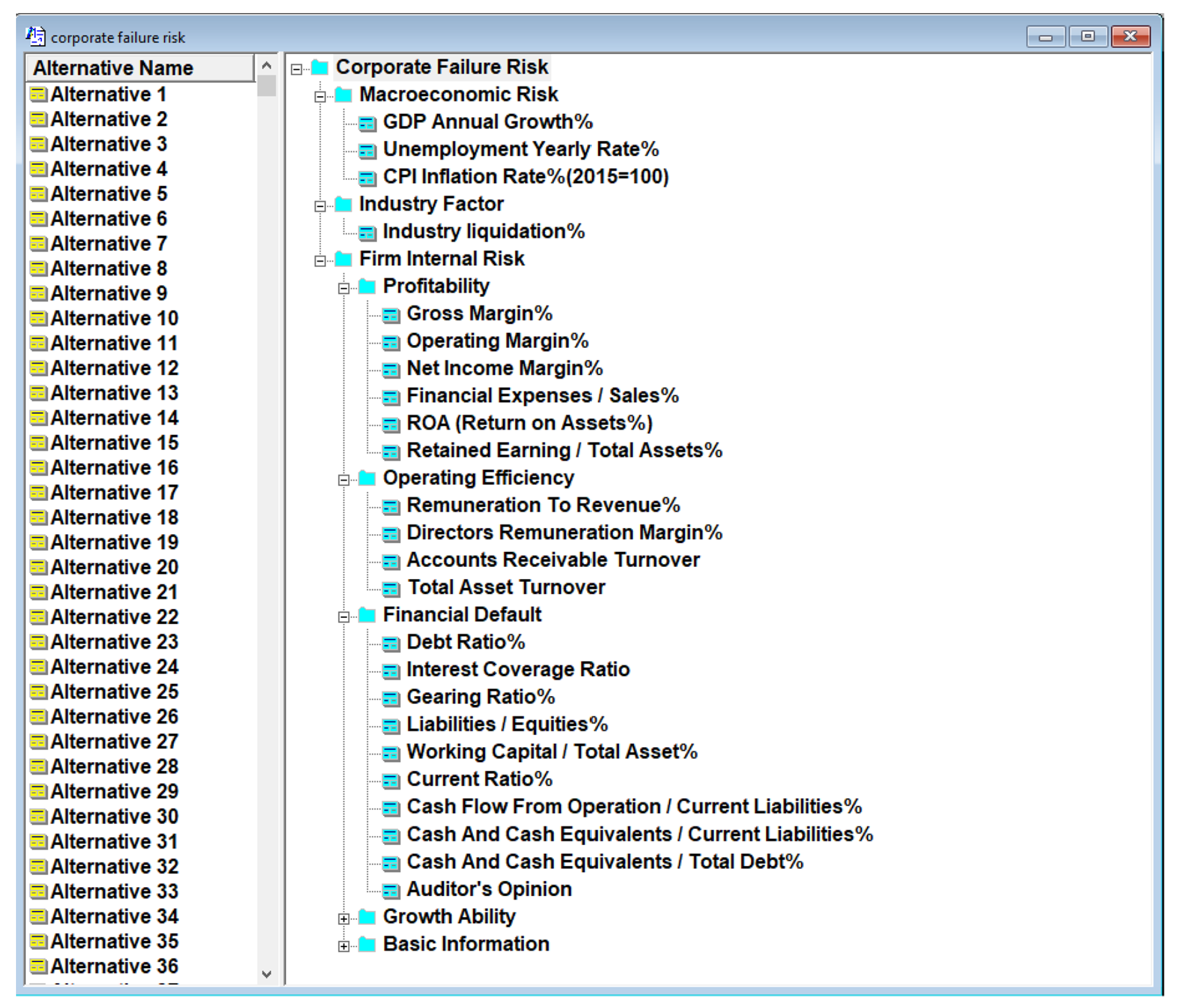
2.2. The Hierarchical Model of Failure Risk Assessment for KIS
2.3. The ER Approach and IDS Software
2.4. The Measurement and Weight of Attributes
3. The Application of the Corporate Risk Assessment Model and Results
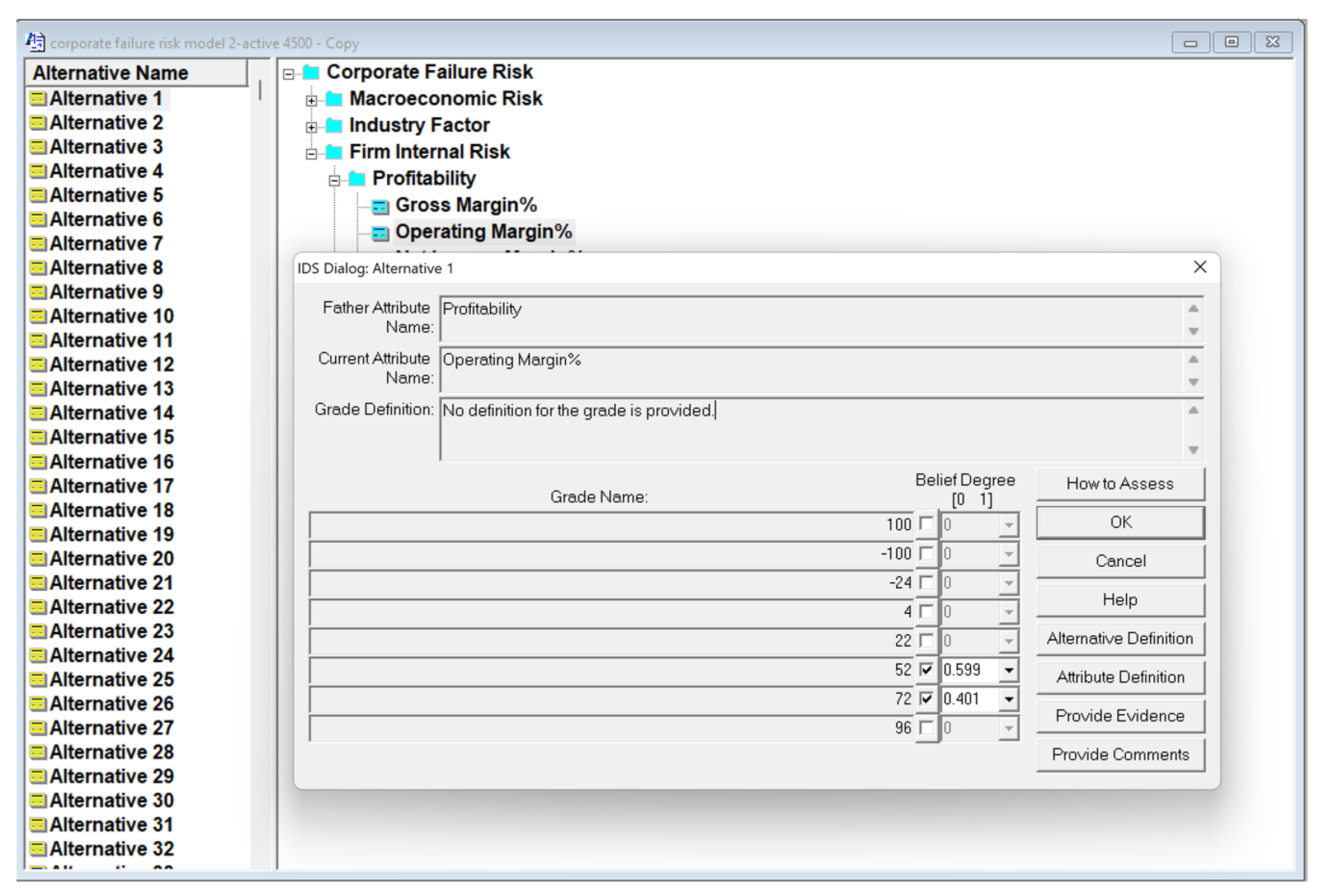
3.1. IDS Application
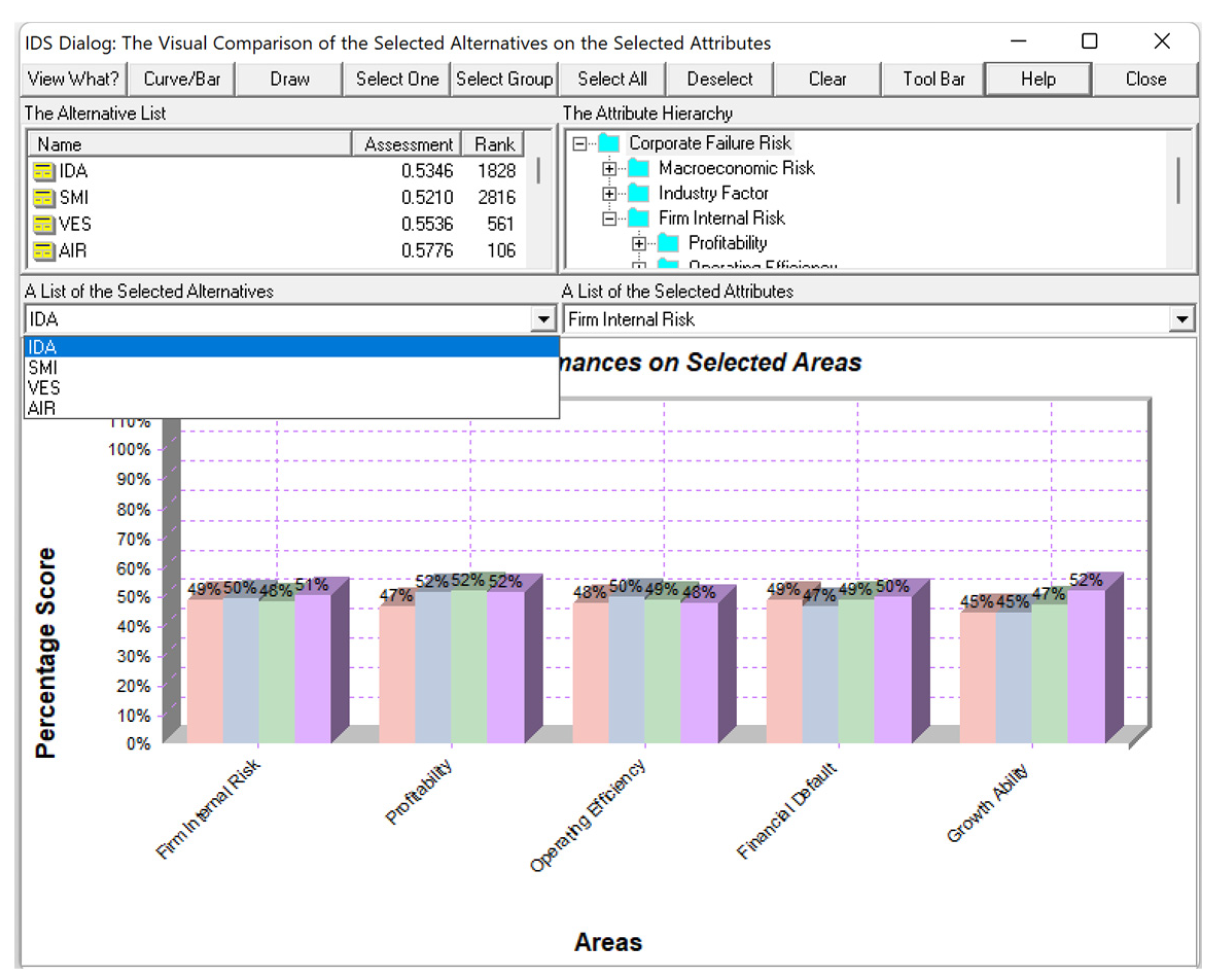
3.2. Result Discussion
4. Conclusions
Author Contributions
Funding
Institutional Review Board Statement
Informed Consent Statement
Data Availability Statement
Conflicts of Interest
Appendix A

| Level 2 Attributes | Level 3 Attributes | Level 4 Attributes | Defination | Measurement |
|---|---|---|---|---|
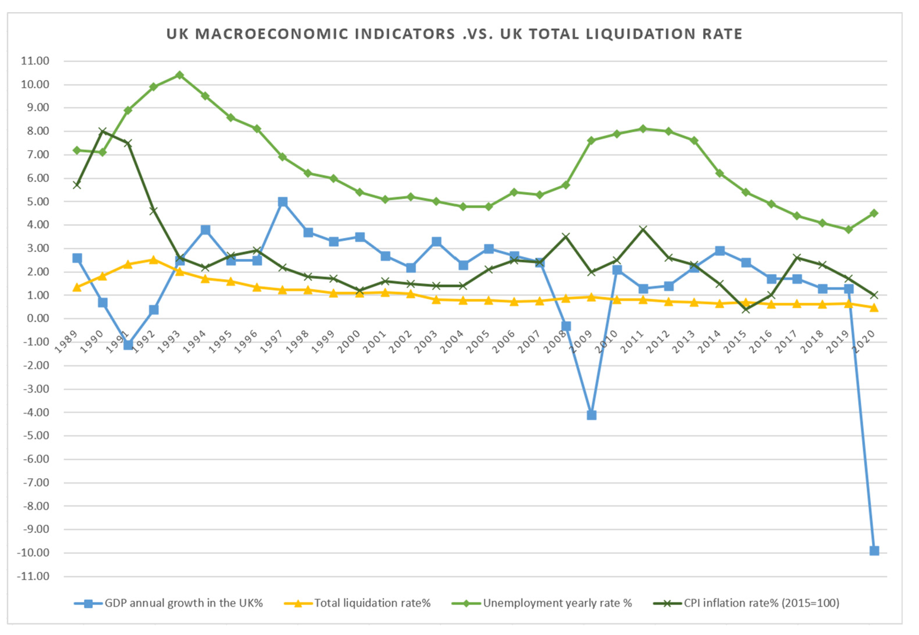
| Macroeconomic Risk(ω = 0.1) | GDP Annual Growth% (gross domestic product growth) (ω = 0.33) | The greater the GDP growth rate, the better the country’s economic development. The two consecutive quarters or more of negative GDP growth means that the economy is in recession (Year on Year growth). | GDPG ≤ 0 economic decline GDPG > 0 economic growth | |
| Unemployment Yearly Rate% (ω = 0.33) | It equals to the No. of people who are without work/labour force of an economy. An increase in the unemployment rate is a signal of economic weakness, which can cause the government to loosen its monetary policy in order to stimulate economic growth; on the contrary, a fall in the unemployment rate will lead to inflation, causing the central bank to tighten its monetary policy and reduce money supply. | Minimum value = 3 Maximum value = 12 During a economic recession, the unemployment rate is higher. | ||
| CPI Inflation Rate% (2015 = 100) (consumer price index change) (ω = 0.33) | CPI refers to the current cost of market basket compared with the base period. The CPI Inflation Rate means the value change over 12 months, which is used to measure the level of national inflation. | Minimum value = 0.4 Maximun value = 8.0 A high CPI inflation rate bad for economy. | ||
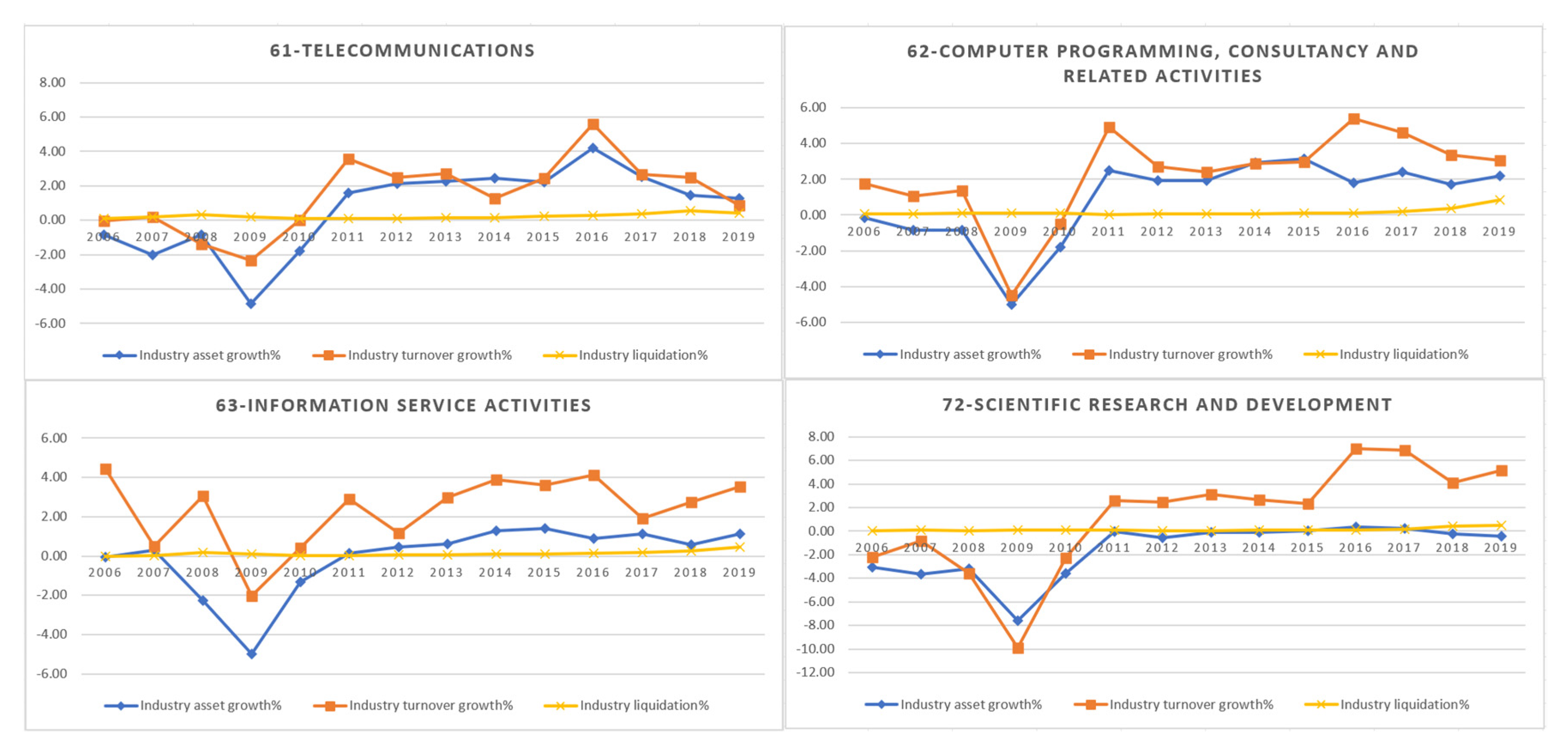
| Industry Factor (ω = 0.1) | Industry liquidation% (ω = 1) | It means the No. of liquidated firms as a percentage of total companies in the industry. (The median values of the four sub-industries are used in the model) | Best value = 0 Worst value = 1 The higher the industry liquidation rate, the greater the probability of company bankruptcy. | |
| Firm Internal Risk (ω = 0.8) | Profitability (ω = 0.167) | Gross Margin% (ω = 0.118) | Gross Profit/Turnover*100 (Fame: Turnover = Revenue) It reflects the initial profitability of the main business product or service. Gross Profit is equal to total sales or revenue minus cost of sales, If the company does not have enough gross profit, it may not be able to make up for the subsequent period expenses (e.g., administration expenses, distribution expenses) and then suffer losses. | GPM% = −100 47% low risk, 53% high risk; GPM% = −10 38.1% low risk, 61.9% high risk; GPM% = 12 43.5% low risk, 56.5% high risk; GPM% = 48 47.8% low risk, 52.2% high risk; GPM% = 62 54.4% low risk, 45.6% high risk; GPM% = 88 50% low risk, 50% high risk; GPM% = 100 46.6% low risk, 53.4% high risk. |
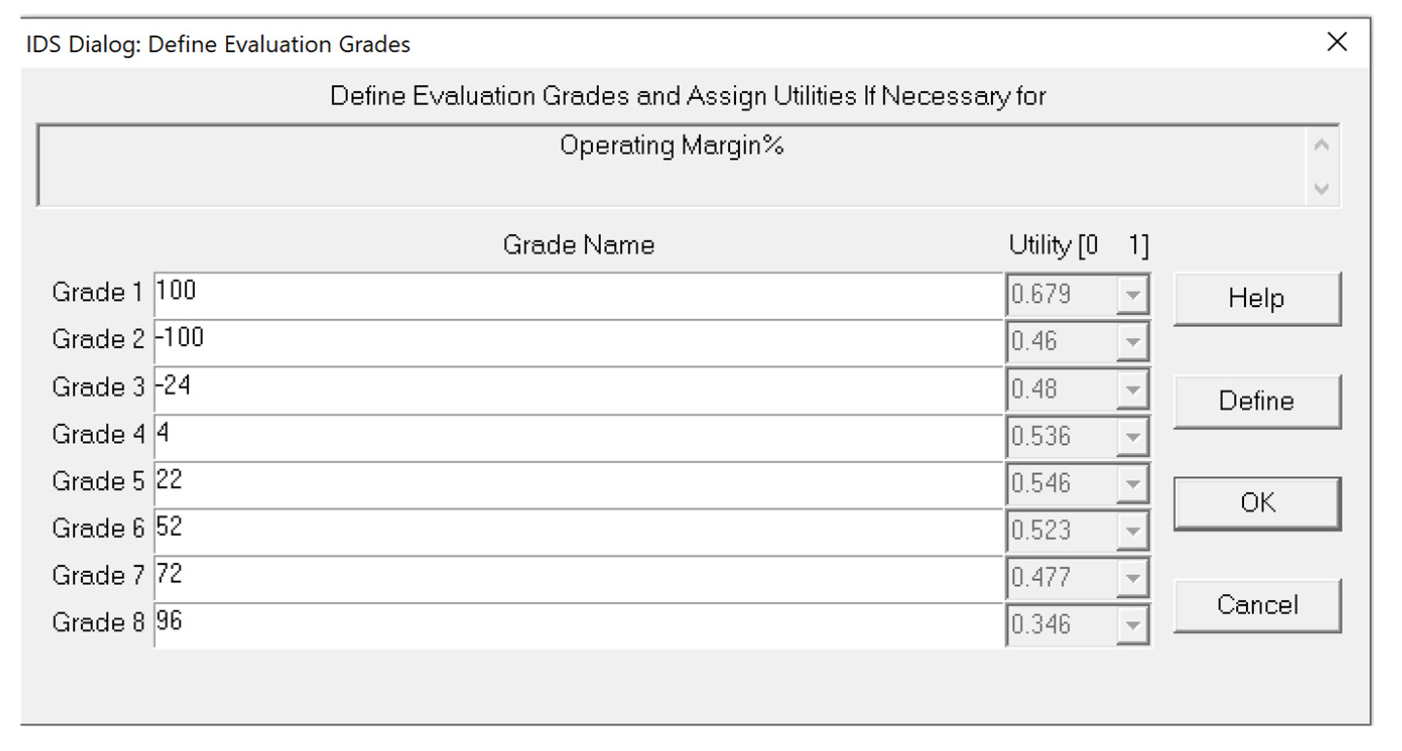
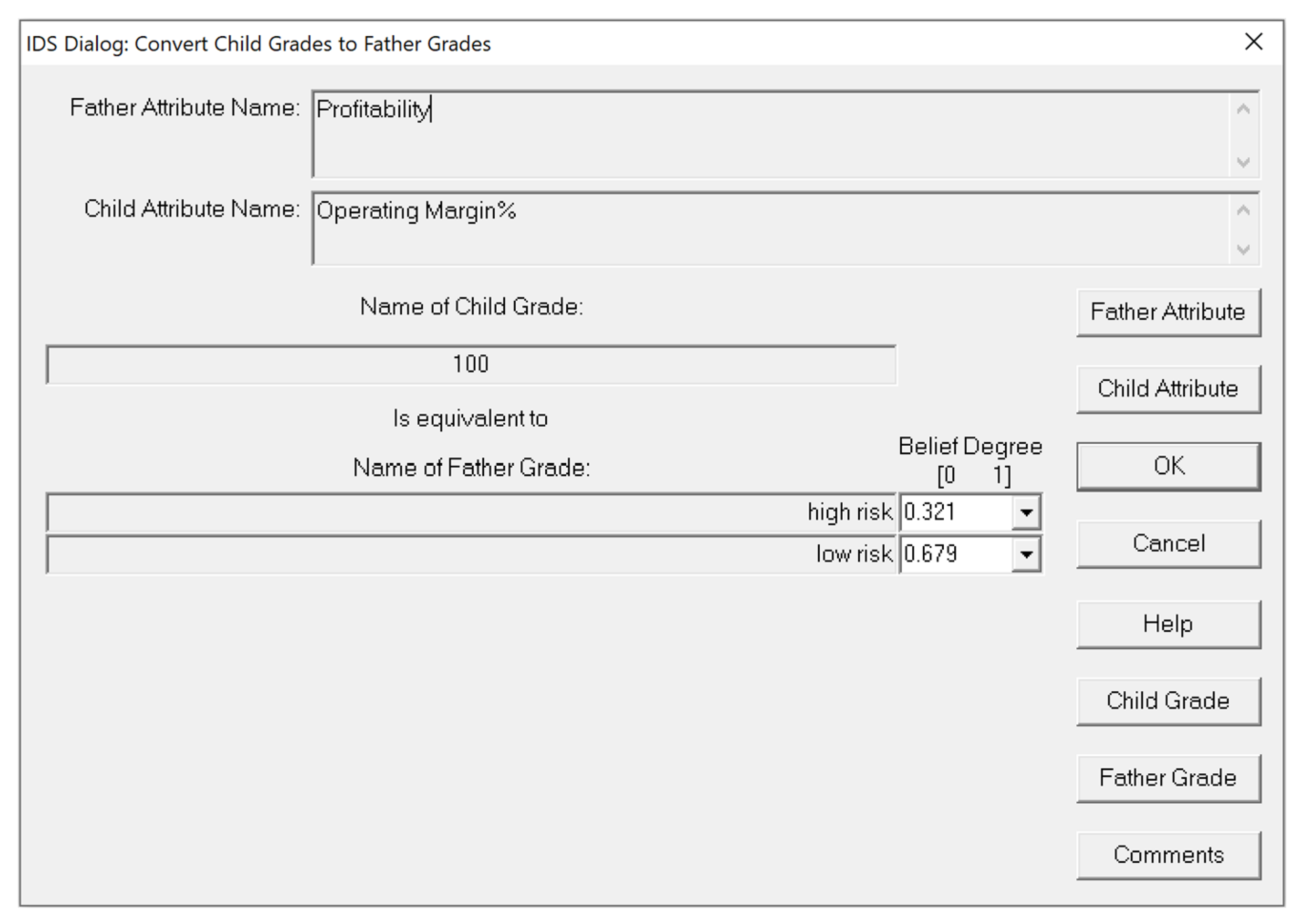
| Firm Internal Risk (ω = 0.8) | Profitability (ω = 0.167) | Operating Margin% (ω = 0.118) | Operating Profit/Turnover*100 Operating profit is equal to gross profit minus all subsequent period expense. When consider expense, e.g., administration expense, many companies have a negative value of profit. | OPM% = −100 46% low risk, 54% high risk; OPM% = −24 48% low risk, 52% high risk; OPM% = 4 53.6% low risk, 46.4% high risk; OPM% = 22 54.6% low risk, 45.4% high risk; OPM% = 52 52.3% low risk, 47.7% high risk; OPM% = 72 47.7% low risk, 52.3% high risk; OPM% = 96 34.6% low risk, 65.4% high risk; OPM% = 100 67.9% low risk, 32.1% high risk. |
| Net Income Margin% (ω = 0.235) | Net income/turnover*100 The net income is the balance of the company’s total income minus all costs and expenses. The larger the index, the higher the profitability of the company’s business activities. Comparing gross margin and net income margin, we can find out the risks in the business management, such as if the product pricing is reasonable, or whether the main business cost and other various expenses are too high. | NIM% ∈(−ꝏ, −800] 37.4% low risk, 62.6% high risk; NIM% = −100 46.3% low risk, 53.7% high risk; NIM% = −44 46% low risk, 54% high risk; NIM% = 4 54% low risk, 46% high risk; NIM% = 36 53.4% low risk, 46.6% high risk; NIM% = 60 44.8% low risk, 55.2% high risk; NIM% = 84 36.1% low risk, 63.9% high risk; NIM% ∈ [200, +ꝏ) 33.2% low risk, 66.8% high risk. | ||
| Financial Expenses/Sales% (ω = 0.059) | interest paid/turnover*100 | FES% = 0.01 49.3% low risk, 50.7% high risk; FES% = 0.08 50.7% low risk, 49.3% high risk; FES% = 0.3 44.4% low risk, 55.6% high risk; FES% = 1 37.6% low risk, 62.4% high risk; FES% = 5 43.5% low risk, 56.5% high risk; FES% = 50 44.8% low risk, 55.2% high risk; FES% ∈ [300, +ꝏ) 20.5% low risk, 79.5% high risk. | ||
| Roa(Return On Assets%) (ω = 0.235) | Net Income/Total Asset*100 The return on total assets index assesses the efficiency of asset utilization. In the case of a certain amount of corporate assets, it can be used to analyse the stability of corporate profitability and determine the risks faced by the company. It may also reflect the level of comprehensive management of the enterprise. The higher value of ROA, the better the efficiency of corporate capital utilization and the stronger the profitability. | ROA% ∈ (−ꝏ, −750] 38.5% low risk, 61.5% high risk; ROA% = −200 37.3% low risk, 62.7% high risk; ROA% = −38 39.1% low risk, 60.9% high risk; ROA% = −16 53.9% low risk, 46.1% high risk; ROA% = 4 54.5% low risk, 45.5% high risk; ROA% = 40 46.2% low risk, 53.8% high risk; ROA% = 150 48.3% low risk, 51.7% high risk; ROA% = 300 64% low risk, 36% high risk; ROA% ∈ [1000, +ꝏ) 61.2% low risk, 38.8% high risk. | ||
| Firm Internal Risk (ω = 0.8) | Profitability (ω = 0.167) | Retained Earning/Total Assets% (ω = 0.235) | Retained earning/Total assets*100 (Fame: Retained earning = Profit (Loss) Account) | REA ∈ (−ꝏ, −4000] 32.2% low risk, 67.8% high risk; REA = −300 35.7% low risk, 64.3% high risk; REA = −120 42.4% low risk, 57.6% high risk; REA = −16 49% low risk, 51% high risk; REA = 4 50.7% low risk, 49.3% high risk; REA = 56 56.2% low risk, 43.8% high risk; REA = 90 47.9% low risk, 52.1% high risk REA ∈ [100, +ꝏ) 55.9% low risk, 44.1% high risk. |
| Operating Efficiency (ω = 0.167) | Remuneration To Revenue% (ω = 0.286) | Remuneration/Turnover*100 | RER% = 2 43.4% low risk, 56.6% high risk; RER% = 20 55.4% low risk, 44.6% high risk; RER% = 50 52.6% low risk, 47.4% high risk; RER% = 84 49.2% low risk, 50.8% high risk; RER% = 96 38.2% low risk, 61.8% high risk; RER% = 200 34.6% low risk, 65.4% high risk; RER% ∈ [1000, +ꝏ) 26.5% low risk, 73.5% high risk. | |
| Directors Remuneration Margin% (ω = 0.142) | Directors remuneration/remuneration% | DRR% = 1 55.8% low risk, 44.2% high risk; DRR% = 9 53.7% low risk, 46.3% high risk; DRR% = 16 47% low risk, 53% high risk; DRR% = 25 41.4% low risk, 58.6% high risk; DRR% = 80 48.5% low risk, 51.5% high risk; DRR% = 100 45.6% low risk, 54.4% high risk; DRR% ∈ [200, +ꝏ) 100% low risk, 0% high risk. | ||
| Accounts Receivable Turnover (ω = 0.286) | Turnover/Trade Debtors It measures the realization speed of the company’s accounts receivable. The higher the index, the stronger liquidity of assets and the lower bad debt losses. However, too high accounts receivable turnover rate limits the company’s sales scale. | ART = 1 57.4% low risk, 42.6% high risk; ART = 3 50% low risk, 50% high risk; ART = 5.5 50.8% low risk, 49.2% high risk; ART = 9.5 52.5% low risk, 47.5% high risk; ART = 12 42.6% low risk, 57.4% high risk; ART = 20 48.1% low risk, 51.9% high risk; ART = 40 42.7% low risk, 57.3% high risk; ART = 90 43.7% low risk, 56.3% high risk; ART ∈ [200, +ꝏ) 56.7% low risk, 43.3% high risk. | ||
| Firm Internal Risk (ω = 0.8) | Operating Efficiency (ω = 0.167) | Total Asset Turnover (ω = 0.286) | turnover/total assets It can be applied to evaluate the use efficiency of all assets of the enterprise. The utilization of the enterprise assets could be improved by increasing income or reducing assets. The larger the better. | TAT = 0.1 48.2% low risk, 51.8% high risk; TAT = 1.8 50.7% low risk, 49.3% high risk; TAT = 4.5 49.9% low risk, 50.1% high risk; TAT = 8 49.5% low risk, 50.5% high risk; TAT = 20 53% low risk, 47% high risk; TAT = 80 55.4% low risk, 44.6% high risk; TAT ∈ [100, +ꝏ) 55.5% low risk, 44.5% high risk. |
| Financial Default (ω = 0.333) | Debt Ratio% (ω = 0.143) | Total liabilities/Total Assets It indicates the proportion of funds provided by creditors in total assets. The scale of corporate debt should be kept within a reasonable range. When the debt ratio is greater than 100, it shows that the company is insolvent and the owner’s equity is negative. | DR% = 2 61.1% low risk, 38.9% high risk; DR% = 8 43.5% low risk, 56.5% high risk; DR% = 42 55.1% low risk, 44.9% high risk; DR% = 86 53.1% low risk, 46.9% high risk; DR% = 100 45.3% low risk, 54.7% high risk; DR% = 230 40.3% low risk, 59.7% high risk; DR% = 500 44.8% low risk, 55.2high risk; DR% = 3000 39.9% low risk, 60.1% high risk; DR% ∈ [15,000, +ꝏ) 33.1% low risk, 66.9% high risk; | |
| Interest Coverage Ratio (ω = 0.036) | Profit (Loss) before Interest paid/Interest Paid It is used to assess the company’s ability to pay interest expenses. A low value means that the company’s profits can only be barely used to pay interest on liabilities, which further shows that the company’s solvency is weak. | ICR = −50 35.6% low risk, 64.4% high risk; ICR = −10 29.1% low risk, 70.9% high risk; ICR = −4 43.1% low risk, 56.9% high risk; ICR = 2 49.4% low risk, 50.6% high risk; ICR = 17 43.4% low risk, 56.6% high risk; ICR = 40 43.1% low risk, 56.9% high risk; ICR ∈ (200, +ꝏ) 55.3% low risk, 44.7% high risk. | ||
| Gearing Ratio% (ω = 0.143) | (Short Term Loans & Overdrafts + Long Term Liabilities)/Shareholders Funds *100 It is an indicator used to evaluate the rationality of capital structure and the company’s long-term solvency. Low debt means that the company does not make full use of the leverage effect, thereby limiting the expansion of the company. However, high debt brings higher risks to creditors and investors. | GR% = 1 50.7% low risk, 49.3% high risk; GR% = 10 50.7% low risk, 49.3% high risk; GR% = 14 51.1% low risk, 48.9% high risk; GR% = 34 55.2% low risk, 44.8% high risk; GR% = 90 51.4% low risk, 48.6% high risk; GR% = 250 52.5% low risk, 47.5% high risk; GR% ∈ [800, +ꝏ) 50.3% low risk, 49.7% high risk. | ||
| Firm Internal Risk (ω = 0.8) | Financial Default (ω = 0.333) | Liabilities/Euqities% (ω = 0.071) | liabilities/euqities*100 | LE% ∈ (−ꝏ, −1000) 50.3% low risk, 49.7% high risk; LE% = −550 41% low risk, 59% high risk; LE% = −100 42.1% low risk, 57.9% high risk; LE% = 5 47.1% low risk, 52.9% high risk; LE% = 90 55.9% low risk, 44.1% high risk; LE% = 150 56% low risk, 44% high risk; LE% = 550 49.3% low risk, 50.7% high risk; LE% = 1000 54.7% low risk, 45.3% high risk; LE% ∈ [5000, +ꝏ) 41.6% low risk, 58.4% high risk. |
| Working Capital/Total Asset% (ω = 0.143) | Working capital/total asset*100 OR (Current Assets-Current Liabilities)/total assets*100 | WCA% = −2000 32.7% low risk, 67.3% high risk; WCA% = −750 45.6% low risk, 54.4% high risk; WCA% = −100 45.1% low risk, 54.9% high risk; WCA% = −15 45.6% low risk, 54.4% high risk; WCA% = 5 51.5% low risk, 48.5% high risk; WCA% = 10 53.6% low risk, 46.4% high risk; WCA% = 60 51.7% low risk, 48.3% high risk; WCA% = 90 43.8% low risk, 56.2% high risk; WCA% = 100 59.2% low risk, 40.8% high risk. | ||
| Current Ratio% (ω = 0.143) | Current Assets/Current Liabilities It means how much current assets can be used to repay each unit of current liabilities. The higher the ratio, the stronger the company’s short-term debt repayment ability, and the less likely that the company will default on their debt. | CR% = 0.1 42.6% low risk, 57.4% high risk; CR% = 0.4 45.9% low risk, 54.1% high risk; CR% = 1 49.7% low risk, 50.3% high risk; CR% = 2 53.1% low risk, 46.9% high risk; CR% = 3 47.1% low risk, 52.9% high risk; CR% = 20 48.3% low risk, 51.7% high risk; CR% = 100 51.1% low risk, 48.9% high risk. | ||
| Cash Flow From Operation/ Current Liabilities% (ω = 0.071) | cash flow from operation/current liabilities*100 It evaluates the company’s ability to repay short-term liabilities from the perspective of cash flow. When the value of this indicator is large, it indicates that the company has sufficient cash flow, which can guarantee the timely repayment of debts. However, if the value is too large, it means that the company has not fully utilized assets and the management efficiency is low. | CAL% ∈ (−ꝏ, −300] 32.1% low risk, 67.9% high risk; CAL% = −30 35.5% low risk, 64.5% high risk; CAL% = 10 59.5% low risk, 40.5% high risk; CAL% = 70 53.4% low risk, 46.6% high risk; CAL% = 150 40.2% low risk, 59.8% high risk; CAL% ∈ [500, +ꝏ) 44% low risk, 56% high risk. | ||
| Firm Internal Risk (ω = 0.8) | Financial Default (ω = 0.333) | Cash And Cash Equivalents/ Current Liabilities% (ω = 0.143) | cash and cash equivalents/current liabilities*100 | CCL% = 1 34.2% low risk, 65.8% high risk; CCL% = 4 38.1% low risk, 61.9% high risk; CCL% = 10 48.9% low risk, 51.1% high risk; CCL% = 78 55% low risk, 45% high risk; CCL% = 120 60.1% low risk, 39.9% high risk; CCL% = 400 54.2% low risk, 45.8% high risk; CCL% ∈ (5000, +ꝏ) 48.8% low risk, 51.2% high risk. |
| Cash And Cash Equivalents/ Total Debt% (ω = 0.036) | increased cash and cash equivalents/total debt*100 | CCD% ∈ (−ꝏ, −100] 60.7% low risk, 39.3% high risk; CCD% = −30 38.6% low risk, 61.4% high risk; CCD% = 5 46.1% low risk, 53.9% high risk; CCD% = 25 59.1% low risk, 40.9% high risk; CCD% = 85 47.6% low risk, 52.4% high risk; CCD% ∈ [200, +ꝏ) 49.1% low risk, 50.9% high risk. | ||
| Auditor’S Opinion (ω = 0.071) | It is an opinion expressed by an independent auditor on whether the company’s financial statements meet the standards. | AO = Qualified 16% low risk, 84% high risk; AO = Not audited/unknown 55% low risk, 45% high risk; AO = Unqualified 46% low risk, 54% high risk. | ||
| Growth Ability (ω = 0.167) | Revenue Growth% (ω = 0.308) | Revenue growth-1 year% | RG% = −100 40.6% low risk, 59.4% high risk; RG% = −20 42.2% low risk, 57.8% high risk; RG% = −14 50.8% low risk, 49.2% high risk; RG% = 5 54.8% low risk, 45.2% high risk; RG% = 20 58.3% low risk, 41.7% high risk; RG% = 30 61% low risk, 39% high risk; RG% = 80 51.5% low risk, 48.5% high risk; RG% ∈ [200, +ꝏ) 50.3% low risk, 49.7% high risk. | |
| Asset Growth% (ω = 0.154) | Asset growth-1 year% | AG% = −100 45.4% low risk, 54.6% high risk; AG% = −20 47.1% low risk, 52.9% high risk; AG% = −14 53.5% low risk, 46.5% high risk; AG% = 2 56.3% low risk, 43.7% high risk; AG% = 20 54.3% low risk, 45.7% high risk; AG% = 30 46.3% low risk, 53.7% high risk; AG% ∈ [200, +ꝏ) 46.8% low risk, 53.2% high risk. | ||
| Firm Internal Risk (ω = 0.8) | Growth Ability (ω = 0.167) | Intangible Assets/ Total Assets% (ω = 0.076) | intangible assets/total assets*100 | ITA% = −1 57.4% low risk, 42.6% high risk; ITA% = 1 59.6% low risk, 40.4% high risk; ITA% = 5 52.1% low risk, 47.9% high risk; ITA% = 10 40.3% low risk, 59.7% high risk; ITA% = 45 47.8% low risk, 52.2% high risk; ITA% = 100 43.3% low risk, 56.7% high risk. |
| Cash Flow From Operations/Sales% (ω = 0.154) | Cash Flow From Operations/Sales *100 It represents the net cash flow from operating activities per unit of sales revenue. | CAS% ∈ (−ꝏ, −100] 28.7% low risk, 71.3% high risk; CAS% = −10 39.1% low risk, 60.9% high risk; CAS% = 5 59.9% low risk, 40.1% high risk; CAS% = 15 59.6% low risk, 40.4% high risk; CAS% = 50 38% low risk, 62% high risk; CAS% ∈ [250, +ꝏ) 54.1% low risk, 45.9% high risk. | ||
| Cash And Cash Equivalents/Current Asset% (ω = 0.308) | cash and cash equivalents/current asset*100 It examines the proportion of cash to current asset. The larger the value the more stable the development and the lower the operating risk. | CCA% = 1 37.1% low risk, 62.9% high risk; CCA% = 4 40.8% low risk, 59.2% high risk; CCA% = 32 49.9% low risk, 50.1% high risk; CCA% = 54 56.2% low risk, 43.8% high risk; CCA% = 96 54.7% low risk, 45.3% high risk; CCA% = 100 61.1% low risk, 38.9% high risk. | ||
| Basic Information (ω = 0.167) | Average Age Of Directors% (ω = 0.111) | DA% = 18 54.8% low risk, 45.2% high risk; DA% = 45 51.2% low risk, 48.8% high risk; DA% = 52 43.5% low risk, 56.5% high risk; DA% = 57 48.1% low risk, 51.9% high risk; DA% = 66 57.7% low risk, 42.3% high risk; DA% = 93 62.4% low risk, 37.6% high risk. | ||
| Women On Board% (ω = 0.111) | WOB% = 1 47.8% low risk, 52.2% high risk; WOB% = 10 47% low risk, 53% high risk; WOB% = 20 51.6% low risk, 48.4% high risk; WOB% = 40 57.4% low risk, 42.6% high risk; WOB% = 50 61.6% low risk, 38.4% high risk; WOB% =67 53.1% low risk, 46.9% high risk; WOB% = 100 48.6% low risk, 51.4% high risk. | |||
| Firm Internal Risk (ω = 0.8) | Basic Information (ω = 0.167) | Firm Size(No. Of Employee) (ω = 0.222) | NEM = 1 40.6% low risk, 59.4% high risk; NEM = 3 46.8% low risk, 53.2% high risk; NEM = 10 43.7% low risk, 56.3% high risk; NEM = 50 43.1% low risk, 56.9% high risk; NEM = 55 54.7% low risk, 45.3% high risk; NEM = 200 55.8% low risk, 44.2% high risk; NEM = 250 57.1% low risk, 42.9% high risk; NEM = 900 61.9% low risk, 38.1% high risk; NEM = 3000 96.3% low risk, 3.7% high risk. | |
| Company Age (ω = 0.222) | CA% = 1 23.1% low risk, 76.9% high risk; CA% = 6 34.6% low risk, 65.4% high risk; CA% = 10 55.5% low risk, 44.5% high risk; CA% = 26 63.5% low risk, 36.5% high risk; CA% = 40 80.7% low risk, 19.3% high risk; CA% = 120 68.7% low risk, 31.3% high risk. | |||
| Firm Size (Ln Assets) (ω = 0.222) | LNA% = 1 77.9% low risk, 22.1% high risk; LNA% = 8 74% low risk, 26% high risk; LNA% = 11 47.6% low risk, 52.4% high risk; LNA% = 14 38.6% low risk, 61.4% high risk; LNA% = 16 50.2% low risk, 49.8% high risk; LNA% = 20 59.7% low risk, 40.3% high risk; LNA% = 26 44.9% low risk, 55.1% high risk. | |||
| No. Of Subsidiaries (ω = 0.111) | NSB% = 1 59.8% low risk, 40.2% high risk; NSB% = 2 59.8% low risk, 40.2% high risk; NSB% = 4 94.1% low risk, 5.9% high risk; NSB% = 10 87.4% low risk, 12.6% high risk; NSB% = 60 69.8% low risk, 30.2% high risk; NSB% = 250 100% low risk, 0% high risk. |
References
- Agarwal, Vineet, and Richard Taffler. 2008. Comparing the performance of market-based and accounting-based bankruptcy prediction models. Journal of Banking and Finance 32: 1541–51. [Google Scholar] [CrossRef] [Green Version]
- Alaka, Hafiz A., Lukumon O. Oyedele, Hakeem A. Owolabi, Vikas Kumar, Saheed O. Ajayi, Olugbenga O. Akinade, and Muhammad Bilal. 2018. Systematic review of bankruptcy prediction models: Towards a framework for tool selection. Expert Systems with Applications 94: 164–84. [Google Scholar] [CrossRef]
- Altman, Edward I., Gabriele Sabato, and Nicholas Wilson. 2010. The value of non-financial information in small and medium-sized enterprise risk management. Journal of Credit Risk 6: 95–127. [Google Scholar] [CrossRef] [Green Version]
- Ansari, Abdollah, Ibrahim Said Ahmad, Azuraliza Abu Bakar, and Mohd Ridzwan Yaakub. 2020. A hybrid metaheuristic method in training artificial neural network for bankruptcy prediction. IEEE Access 8: 176640–50. [Google Scholar] [CrossRef]
- Barboza, Flavio, Herbert Kimura, and Edward Altman. 2017. Machine learning models and bankruptcy prediction. Expert Systems with Applications 83: 405–17. [Google Scholar] [CrossRef]
- Barreda, Albert A., Yoshimasa Kageyama, Dipendra Singh, and Sandra Zubieta. 2016. Hospitality Bankruptcy in United States of America: A Multiple Discriminant Analysis-Logit Model Comparison. Journal of Quality Assurance in Hospitality & Tourism 18: 86–106. [Google Scholar]
- Bellovary, Jodi L., Don E. Giacomino, and Michael D. Akers. 2007. A review of bankruptcy prediction studies: 1930 to present. Journal of Financial Education 33: 1–42. [Google Scholar]
- Belton, Valerie, and Theodor J. Stewart. 2002. Multiple Criteria Decision Analysis—An Integrated Approach. Dordrecht: Kluwer Academic Publishers, ISBN 0-7923-7505-X. [Google Scholar]
- Bhattacharjee, Arnab, and Jie Han. 2014. Financial distress of Chinese firms: Microeconomic, macroeconomic and institutional influences. China Economic Review 30: 244–62. [Google Scholar] [CrossRef]
- Bromiley, Philip, Michael McShane, Anil Nair, and Elzotbek Rustambekov. 2015. Enterprise risk management: Review, critique, and research directions. Long Range Planning 48: 265–76. [Google Scholar] [CrossRef] [Green Version]
- Chapman, Robert J. 2011. Simple Tools and Techniques for Enterprise Risk Management. Hoboken: John Wiley & Sons. [Google Scholar]
- Company Insolvencies. 2021. Company Insolvencies in Q4 2020 Were Lower Compared to That of Q4 2019 for England, Wales, Scotland and Northern IRELAND. Available online: https://www.companyrescue.co.uk/guides-knowledge/news/company-insolvencies-in-q4-2020-were-lower-compared-to-that-of-q4-2019-for-england-wales-scotland-and-northern-ireland-4628/ (accessed on 29 January 2021).
- Da Silva Etges, Ana Paula Beck, and Marcelo Nogueira Cortimiglia. 2019. A systematic review of risk management in innovation-oriented firms. Journal of Risk Research 22: 364–81. [Google Scholar] [CrossRef]
- Eurostat. 2016. Glossary: Knowledge-Intensive services (KIS). Available online: https://ec.europa.eu/eurostat/statistics-explained/index.php?title=Glossary:Knowledge-intensive_services_(KIS) (accessed on 2 October 2020).
- Gepp, Adrian, and Kuldeep Kumar. 2015. Predicting financial distress: A comparison of survival analysis and decision tree techniques. Procedia Computer Science 54: 396–404. [Google Scholar] [CrossRef] [Green Version]
- Habib, Ahsan, Mabel D. Costa, Hedy Jiaying Huang, Md Borhan Uddin Bhuiyan, and Li Sun. 2020. Determinants and consequences of financial distress: Review of the empirical literature. Accounting and Finance 60: 1023–75. [Google Scholar] [CrossRef]
- Hazak, Aaro, and Kadri Männasoo. 2007. Indicators of Corporate Default: An EU Based Empirical Study. Eesti Pank: Tallinn. [Google Scholar]
- Holton, Glyn A. 2004. ‘Defining risk’. Financial Analysts Journal 60: 19–25. [Google Scholar] [CrossRef] [Green Version]
- Huang, Yu-Pei, and Meng-Feng Yen. 2019. A new perspective of performance comparison among machine learning algorithms for financial distress prediction. Applied Soft Computing 83: 105663. [Google Scholar] [CrossRef]
- Jackson, Richard H.G., and Anthony Wood. 2013. The performance of insolvency prediction and credit risk models in the UK: A comparative study. The British Accounting Review 45: 183–202. [Google Scholar] [CrossRef]
- Jayasekera, Ranadeva. 2018. Prediction of company failure: Past, present and promising directions for the future. International Review of Financial Analysis 55: 196–208. [Google Scholar] [CrossRef]
- Khoja, Layla, Maxwell Chipulu, and Ranadeva Jayasekera. 2019. Analysis of financial distress cross countries: Using macroeconomic, industrial indicators and accounting data. International Review of Financial Analysis 66: 101379. [Google Scholar] [CrossRef]
- Lee, Sangjae, and Wu Sung Choi. 2013. A multi-industry bankruptcy prediction model using back-propagation neural network and multivariate discriminant analysis. Expert Systems with Applications 40: 2941–46. [Google Scholar] [CrossRef]
- Lussier, Robert N., and Sanja Pfeifer. 2001. A crossnational prediction model for business success. Journal of Small Business Management 39: 228–39. [Google Scholar] [CrossRef]
- Nyitrai, Tamás. 2019. Dynamization of bankruptcy models via indicator variables. Benchmarking: An International Journal 26: 317–32. [Google Scholar] [CrossRef]
- Oliveira, Manuel D.N.T., Fernando A.F. Ferreira, Guillermo O. Pérez-Bustamante Ilander, and Marjan S. Jalali. 2017. Integrating cognitive mapping and MCDA for bankruptcy prediction in small-and medium-sized enterprises. Journal of the Operational Research Society 68: 985–97. [Google Scholar] [CrossRef]
- Peres, Cândido, and Mário Antão. 2017. The use of multivariate discriminant analysis to predict corporate bankruptcy: A review. Aestimatio-the Ieb International Journal of Finance 14: 108–31. [Google Scholar]
- Ravi Kumar, P., and Vadlamani Ravi. 2007. Bankruptcy prediction in banks and firms via statistical and intelligent techniques—A review. European Journal of Operational Research 180: 1–28. [Google Scholar] [CrossRef]
- Sadgrove, Kit. 2016. The Complete Guide to Business Risk Management. London: Routledge. [Google Scholar]
- Tinoco, Mario Hernandez, and Nick Wilson. 2013. Financial distress and bankruptcy prediction among listed companies using accounting, market and macroeconomic variables. International Review of Financial Analysis 30: 394–419. [Google Scholar] [CrossRef]
- Valaskova, Katarina, Tomas Kliestik, and Maria Kovacova. 2018. Management of financial risks in Slovak enterprises using regression analysis. Oeconomia Copernicana 9: 105–21. [Google Scholar] [CrossRef] [Green Version]
- Velasquez, Mark, and Patrick T. Hester. 2013. An analysis of multi-criteria decision making methods. International Journal of Operations Research 10: 56–66. [Google Scholar]
- Wilson, Nicholas, and Ali Altanlar. 2014. Company failure prediction with limited information: Newly incorporated companies. Journal of the Operational Research Society 65: 252–64. [Google Scholar] [CrossRef]
- Winston, Wayne L. 1994. Operations Research Applications and Algorithms. Pacific Grove: Duxburg Press. [Google Scholar]
- Yang, Jian-Bo. 2001. Rule and utility based evidential reasoning approach for multiple attribute decision analysis under uncertainty. European Journal of Operational Research 131: 31–61. [Google Scholar] [CrossRef]
- Yang, Jian-Bo, and Dong-Ling Xu. 2013. Evidential reasoning rule for evidence combination. Artificial Intelligence 205: 1–29. [Google Scholar] [CrossRef]
- Yang, Jian-Bo, and Dong-Ling Xu. 2017. Inferential modelling and decision making with data. Paper presented at 23rd International Conference on Automation and Computing (ICAC), Huddersfield, UK, September 7–8; pp. 1–6. [Google Scholar]
- Yurdakul, Mustafa, and Yusuf Tansel İç. 2004. AHP approach in the credit evaluation of the manufacturing firms in Turkey. International Journal of Production Economics 88: 269–89. [Google Scholar] [CrossRef]
- Zhao, Zongyuan, Shuxiang Xu, Byeong Ho Kang, Mir Md Jahangir Kabir, Yunling Liu, and Rainer Wasinger. 2015. Investigation and improvement of multi-layer perceptron neural networks for credit scoring. Expert Systems with Applications 42: 3508–16. [Google Scholar] [CrossRef]

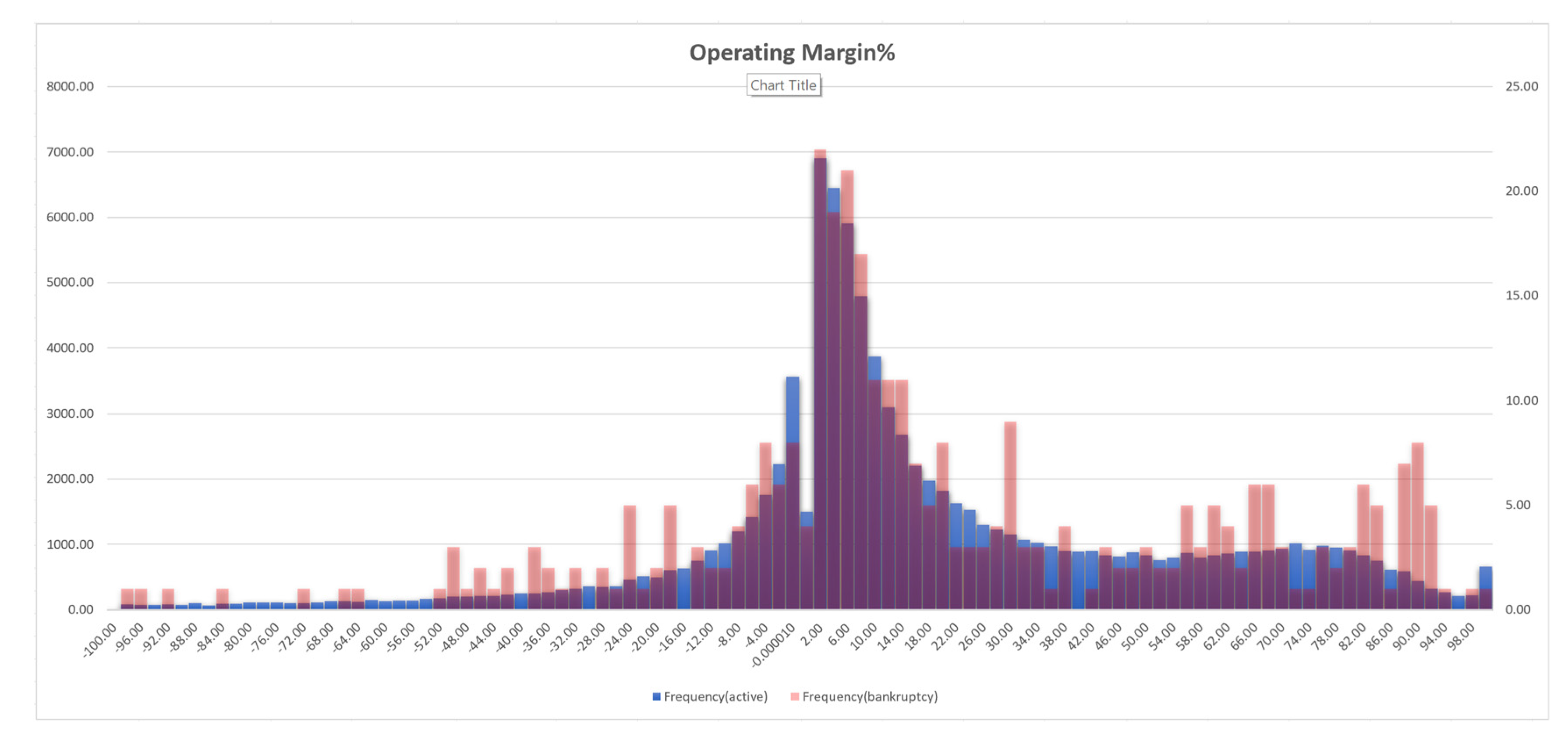


| Frequency | −100 | −24 | 4 | 22 | 52 | 72 | 96 | 100 | Unknown | Total | |
|---|---|---|---|---|---|---|---|---|---|---|---|
| Company Status | low-risk | 2310.27 | 11,584.44 | 38,399.06 | 18,806.35 | 10,935.93 | 9343.78 | 3204.71 | 645.46 | 8662 | 103,892 |
| high-risk | 10.14 | 46.96 | 124.18 | 58.43 | 37.26 | 38.29 | 22.60 | 1.14 | 49 | 388 | |
| Likelihood | −100 | −24 | 4 | 22 | 52 | 72 | 96 | 100 | |||||||||
|---|---|---|---|---|---|---|---|---|---|---|---|---|---|---|---|---|---|
| Company Status | low-risk | 0.022 | 0.460 | 0.112 | 0.480 | 0.370 | 0.536 | 0.181 | 0.546 | 0.105 | 0.523 | 0.090 | 0.477 | 0.031 | 0.346 | 0.006 | 0.679 |
| high-risk | 0.026 | 0.540 | 0.121 | 0.520 | 0.320 | 0.464 | 0.151 | 0.454 | 0.096 | 0.477 | 0.099 | 0.523 | 0.058 | 0.654 | 0.003 | 0.321 | |
Publisher’s Note: MDPI stays neutral with regard to jurisdictional claims in published maps and institutional affiliations. |
© 2022 by the authors. Licensee MDPI, Basel, Switzerland. This article is an open access article distributed under the terms and conditions of the Creative Commons Attribution (CC BY) license (https://creativecommons.org/licenses/by/4.0/).
Share and Cite
Tan, M.-M.; Xu, D.-L.; Yang, J.-B. Corporate Failure Risk Assessment for Knowledge-Intensive Services Using the Evidential Reasoning Approach. J. Risk Financial Manag. 2022, 15, 131. https://doi.org/10.3390/jrfm15030131
Tan M-M, Xu D-L, Yang J-B. Corporate Failure Risk Assessment for Knowledge-Intensive Services Using the Evidential Reasoning Approach. Journal of Risk and Financial Management. 2022; 15(3):131. https://doi.org/10.3390/jrfm15030131
Chicago/Turabian StyleTan, Meng-Meng, Dong-Ling Xu, and Jian-Bo Yang. 2022. "Corporate Failure Risk Assessment for Knowledge-Intensive Services Using the Evidential Reasoning Approach" Journal of Risk and Financial Management 15, no. 3: 131. https://doi.org/10.3390/jrfm15030131
APA StyleTan, M.-M., Xu, D.-L., & Yang, J.-B. (2022). Corporate Failure Risk Assessment for Knowledge-Intensive Services Using the Evidential Reasoning Approach. Journal of Risk and Financial Management, 15(3), 131. https://doi.org/10.3390/jrfm15030131