Article

Is There Any Witching in the Cryptocurrency Market?

1
Department of International Economic Relations, Sumy State University, 40000 Sumy, Ukraine
2
Department of Economics and Entrepreneurship, Sumy National Agrarian University, 40000 Sumy, Ukraine
*
Author to whom correspondence should be addressed.
J. Risk Financial Manag. 2022, 15(2), 92; https://doi.org/10.3390/jrfm15020092
Submission received: 2 February 2022 / Revised: 14 February 2022 / Accepted: 17 February 2022 / Published: 21 February 2022

Abstract

:
This paper explores price effects caused by the expiration of derivatives in the cryptocurrency market. Applying different statistical tests (ANOVA, Mann–Whitney, and t-tests) and econometric methods (the modified cumulative abnormal return approach, regression analysis with dummy variables, and the trading simulation approach) to daily and weekly Bitcoin data over the period 2018–2021, the following hypotheses are tested: (H1) Expiration days create patterns in price behavior in the cryptocurrency market; and (H2) Price patterns can be exploited to generate abnormal profits from trading. The results suggest that expiration effects are only nominally present in the cryptocurrency market. There are differences in returns between expiration-related periods and average returns, but these differences are statistically insignificant. The only case in which an anomaly was detected was related to abnormally high returns during the week of expiration: returns during such weeks were positive in 65% of cases, and were on average 5 times higher than during usual weeks. Trading strategies based on this fact were able to generate results different from those of random trading, with a Sharpe ratio above 1. This is evidence in favor of the existence of a real price anomaly, which contradicts the efficient market hypothesis, and this could be implemented in the practice of traders and investors by creating trading strategies based on detected price effects or special technical analysis indicators to generate trading signals. For academics, these results might provide an opportunity to improve time series forecasting analysis in the case of Bitcoin.

1. Introduction

Expiration of derivatives is a rather routine procedure in financial markets (a lot of contracts expire on a monthly basis). Still, there is a lot of empirical evidence in favor of so-called expiration day effects: abnormally high trading volumes and volatility on these days and during the week prior to the expiration date, as well as patterns in price behavior (Stoll and Whaley 1991).
The expiration effect is based on the idea that market participants adjust their positions around the expiration of options and futures contracts. For example, arbitrageurs liquidate their stock positions around these days and create the order imbalances that arise from unwinding cash positions when futures contracts expire (Stoll and Whaley 1987). Another rationale is stock price manipulation: market participants with large positions in derivative contracts may have incentives to push the underlying market in a certain direction to affect the value of their contracts before they expire (Chow et al. 2003).
According to Yoo (2017), the increase in trading volume on expiration days is mainly due to the increase in the trading volume shares of institutional investors and foreign investors, who are supposed to possess information superiority.
Among expiration days in the US stocks market, there are some rare events referred to as “witching days”, which is when different types of stock market derivatives expire at once. These are the third Fridays of the third month of every quarter (March, June, September, and December). On these days, market index futures, options futures, stock options, and stock futures expire. Intuitively, expiration day effects on days like this should be much stronger. Caporale and Alex (2021) found convincing evidence in favor of abnormal negative returns on these days, and that trading strategies based on this anomaly would provide opportunities to generate abnormal profits from trading.
Bitcoin futures contracts were first introduced in December 2017 by Chicago Mercantile Exchange. The CME Group started trading with listed options on Bitcoin futures on 13 January 2020. As a result, expiration day effects can now be observed in the cryptocurrency market, as well. Nevertheless, no papers on price effects related to expiration days in the cryptocurrency market have been published.
In this paper, we use the latest data from the cryptocurrency market (in this case, Bitcoin) to try to fill this gap. We analyze the price effects in returns caused by expiration days. For this purpose several statistical tests (both parametrical and non-parametrical), as well as special techniques from events studies, are used in this paper. Bitcoin daily and weekly prices are analyzed. Issues related to trading volume and volatility behavior are outside the scope of this paper.
The layout of the paper is as follows: Section 2 reviews the literature. Section 3 describes the data and methodology. Section 4 discusses the empirical results. Section 5 provides concluding remarks.

2. Literature Review

The first evidence found in favor of expiration day effects was provided by Stoll and Whaley (1987), who found abnormal volume and insignificant price movement in the US stock market. Further evidence was found in different stock markets by Schlag (1996), Alkebäck and Hagelin (2004), Chung and Hseu (2008), Hsieh and Ma (2009), Gurgul and Suliga (2019), Singh and Shaik (2020), Batrinca et al. (2020), and others.
Edwards (1988) found volatility growth in the spot market during expiration days of index futures contracts. These observations were confirmed by Arago and Fernandez (2002), Vipul (2005), and others.
However, Schlag (1996) showed that volatility remained unchanged around the expiration of futures contracts in the German stock market. Bollen and Whaley (1999) found no evidence of increased stock market volatility in the Hong Kong Futures Exchange. Chow et al. (2003), who explored the expiration day effect in the Hong Kong stock market, found no abnormal trading volume.
Price effects related to expiration days have also been widely discussed in the academic literature. The most common are negative returns on expiration days (Pope and Yadav 1992) or a day before expiration (Vipul 2005), and price reversal in returns (Stoll and Whaley 1987; Chay and Ryu 2006).
However, these effects are not common to all stock markets. Karolyi (1996), Corredor et al. (2001), and Caihong (2014) found no significant price effects related to expiration days in the Japanese, Hong Kong, or Swedish stock markets, respectively.
As can be seen, existing evidence is mixed because different countries have different markets that apply different methodologies to different time periods.
The cryptocurrency market is a very interesting object of analysis, because it is relatively unexplored. Cryptocurrencies are traded on different exchanges with potentially different prices across different trading venues (Giudici and Pagnottoni 2020), which may be a potential source of inefficiency. Investment portfolio management is very specific in the case of the cryptocurrency market because of the high correlation between instruments (Mazanec 2021). The profitability of technical trading rules (both trend-following and mean-reverting) in the cryptocurrency market is discussed by Resta et al. (2020).
Despite the variety of empirical results for different markets and countries, the expiration day effects in the cryptocurrency market are still unexplored. There has been no discussion or empirical evidence presented related to expiration effects in Bitcoin prices. This paper aims to fill this gap in the academic literature.

3. Data and Methodology

The daily and weekly data for Bitcoin prices (BTCUSD) over the period 1 January 2018–31 December 2021 are used. The data source is the Yahoo Finance (https://finance.yahoo.com/, accessed on 16 February 2022).
Each data set is explored in weekly and daily dimensions divided into 3 periods: witching day periods (day or week when the witching day is present), pre-witching period (day or week before the witching day), and post-witching period (day or week after the witching day).
The following notation is used in the tables to denote them:
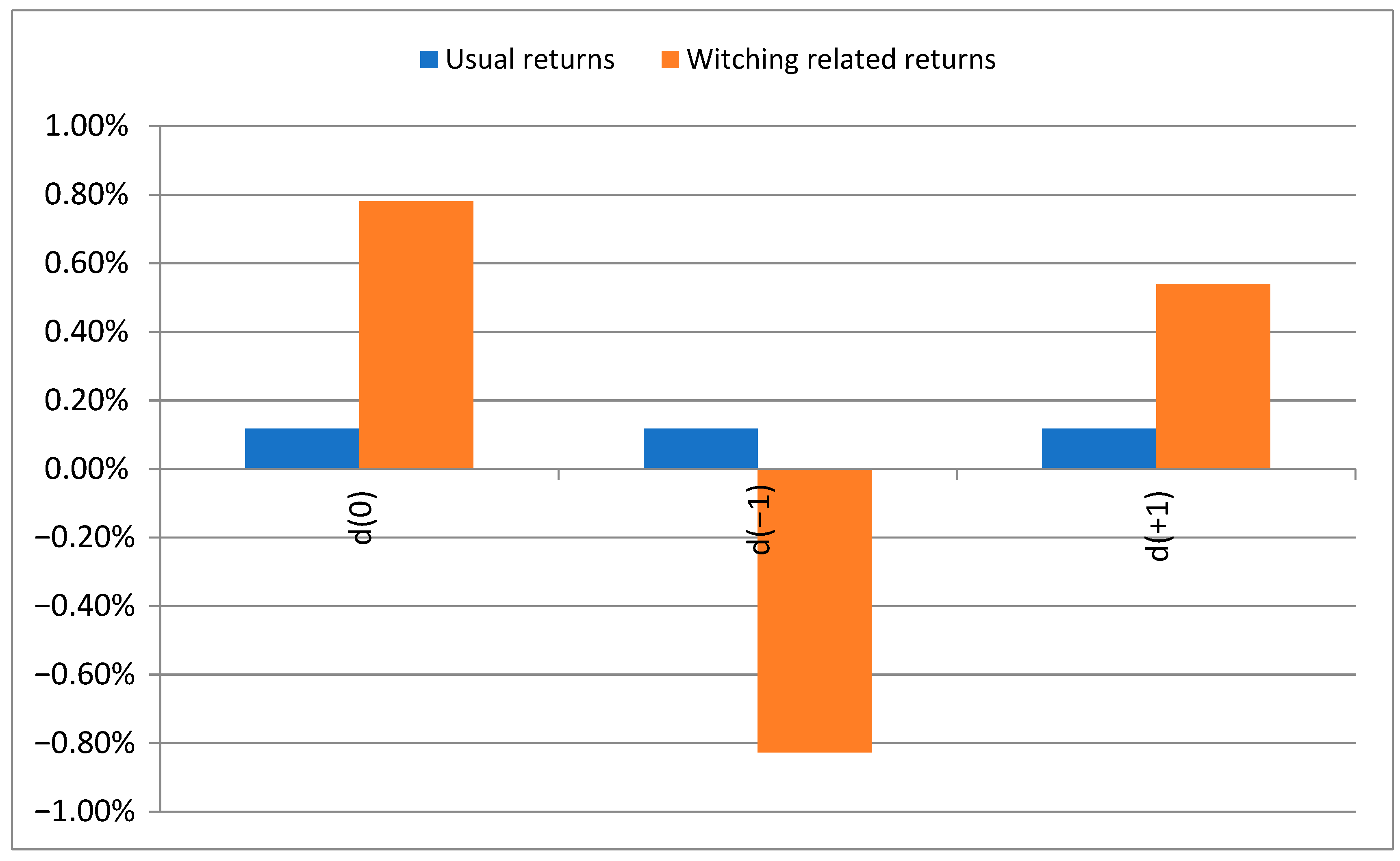
  • d(0)—the expiration day;
  • d(−1)—the day before the expiration day;
  • d(+1)—the day after the expiration day;
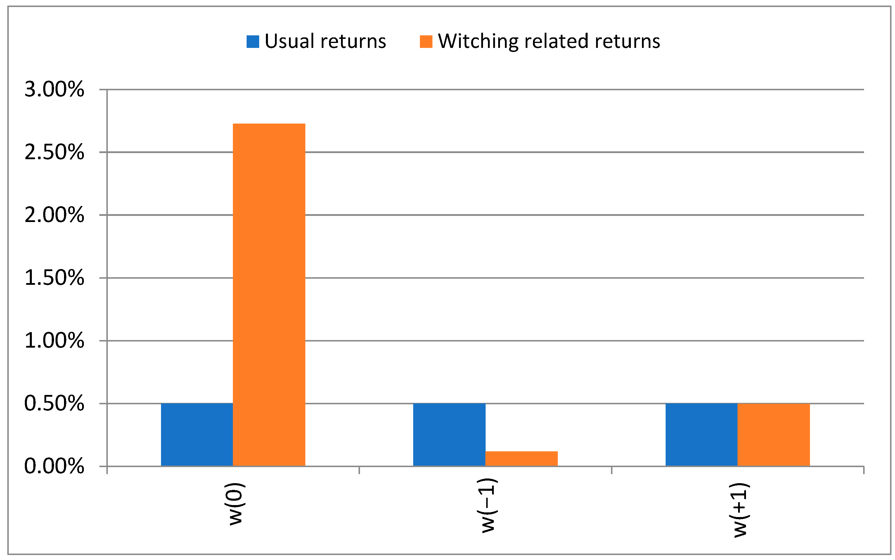
  • w(0)—the week that includes the expiration day;
  • w(−1)—the week before the expiration;
  • w(+1)—the week after the expiration.
The following hypotheses are tested in this paper:
Hypothesis 1 (H1):
Expiration days create patterns in price behavior in the cryptocurrency market.
Hypothesis 2 (H2):
Price patterns can be exploited to generate abnormal profits from trading.
To test H1, various methods and techniques are applied, including parametric tests (Student’s t-test, ANOVA), and non-parametric tests (Mann–Whitney test), the modified cumulative abnormal returns approach, and regression analysis with dummy variables. To test H2, a trading simulation approach is used.
The use of so many different methods makes it possible to avoid methodological bias.
The results of different techniques are summarized, and conclusions are based on integral effect value.
Average analysis provides preliminary evidence as to whether there are differences between returns on normal days and witching days (H1).
Returns are calculated as follows:
R i = ( O p e n i C l o s e i 1 ) × 100 %
where
  • R i —returns on the i-th day in %;
  • O p e n i —open price on the i-th day;
  • C l o s e i —close price on the i-th day.
To make sure the detected differences are statistically significant, several statistical tests are applied. Both parametric and non-parametric tests are used, because of potential differences in data distribution caused by fat tails and kurtosis in returns. The null hypothesis (H0) in each case is that the data on usual days and data related to expiration days belong to the same population, with a rejection of the null suggesting the presence of an anomaly.
A multiple regression analysis with dummy variables is used to provide additional evidence in favor/against H1. It was implemented in the following manner:
R i = a 0 + a 1 D 1 i + ε i
where Ri is the return in period i, a0 is the mean return in a usual period (day or week), a1 is the mean return in an expiration period, Di is a dummy variable equal to 1 in an expiration period and 0 in a usual period, and ε i   is the random error term in the ith period. The sign and statistical significance of the dummy coefficients indicate the existence or not of price effects caused by expiration day.
Expiration days are specific events, although the event studies methodology can be applied to test H1. In this paper, a modified version of the cumulative abnormal returns approach by MacKinlay (1997) is used.
Abnormal returns are defined as follows:
A R i = R i E ( R i )
where R i is the return at time i and E ( R i ) corresponds to the average return computed over the whole sample period, as follows:
E ( R i ) = ( 1 T ) i = 1 T R i
where T is the sample size.
The cumulative abnormal return, denoted as C A R i , is simply the sum of the abnormal returns:
C A R i = i = 1 T A R i
A simple time regression model is implemented on the CARi to determine the presence of a trend. The presence of a trend in the CARi indicates an anomaly. Therefore, a significant p value for the trend term, along with model significance (F test), confirm an anomaly in price behavior related to witching days.
To determine whether a detected anomaly gives rise to exploitable profit opportunities (H2), a trading simulation approach is used.
A trader’s actions are simulated with respect to detected anomalies. Exploitable profit opportunities provide evidence against market efficiency. If a strategy results in more than 50 percent of trades being profitable, as well as a positive total profit, then a market anomaly is detected. The approach used here does not incorporate transaction costs (spread, fees to the broker or bank, swaps, etc.), and only serves as a proxy for actual trading. Nevertheless, it is informative regarding real trading, given that transaction costs are not as essential nowadays as they have been previously. Thanks to the development of the Internet and high-frequency trading, spreads tend to be small, typically ranging between 0.01% and 0.02%. Banking and broker fees can affect profitability in the case of a small number of trades. However, when there are dozens of trades (as in this paper), banking and broker fees become insignificant (this is the so-called scale effect in trading). Therefore, this analysis can shed light on the profitability of anomaly-based trading strategies, even though it overlooks transaction costs.
The following procedure for trading simulation is used. First, the % Result from each trade is defined as follows:
%   r e s u l t = 100 % × P o p e n P c l o s e
where
  • P o p e n —opening price
  • P c l o s e —closing price
Next, the sum of results from each deal is calculated. A positive total financial result from trading indicates the presence of exploitable profits based on that specific price effect. A negative total financial result indicates the opposite. To prove that the generated results differ from random trading, a t-test is carried out. This compares the means of two samples in order to test whether these means originate from the same population. In our case, the first is the average profit/loss factor of one trade applying the trading strategy, and the second is equal to zero, because random trading (without transaction costs) should generate zero profit. A failure to reject H0 (means are the same in both samples) in this instance indicates that the specific anomaly does not provide exploitable profit opportunities.
An additional technique for analyzing the risk-adjusted efficiency of the trading strategy is the use of the Sharpe Ratio.
S h a r p e   r a t i o = R s R f s
where
  • R s —annual profit of trading strategy in %;
  • R f —risk-free rate (2% is used for calculation purposes in this paper—the average value of US 10-year treasury during the period of analysis);
  • s —standard deviation of trade results in %.
The Sharpe ratio is applied instead of Sortino’s ratio because it is more commonly used, making it easier to compare our results with existing alternatives.

4. Empirical Results

The full empirical results for the daily and weekly data are presented in Appendix A and Appendix B, respectively.

4.1. Daily Data

Overall results for usual days and expiration-related days are presented in Table 1.
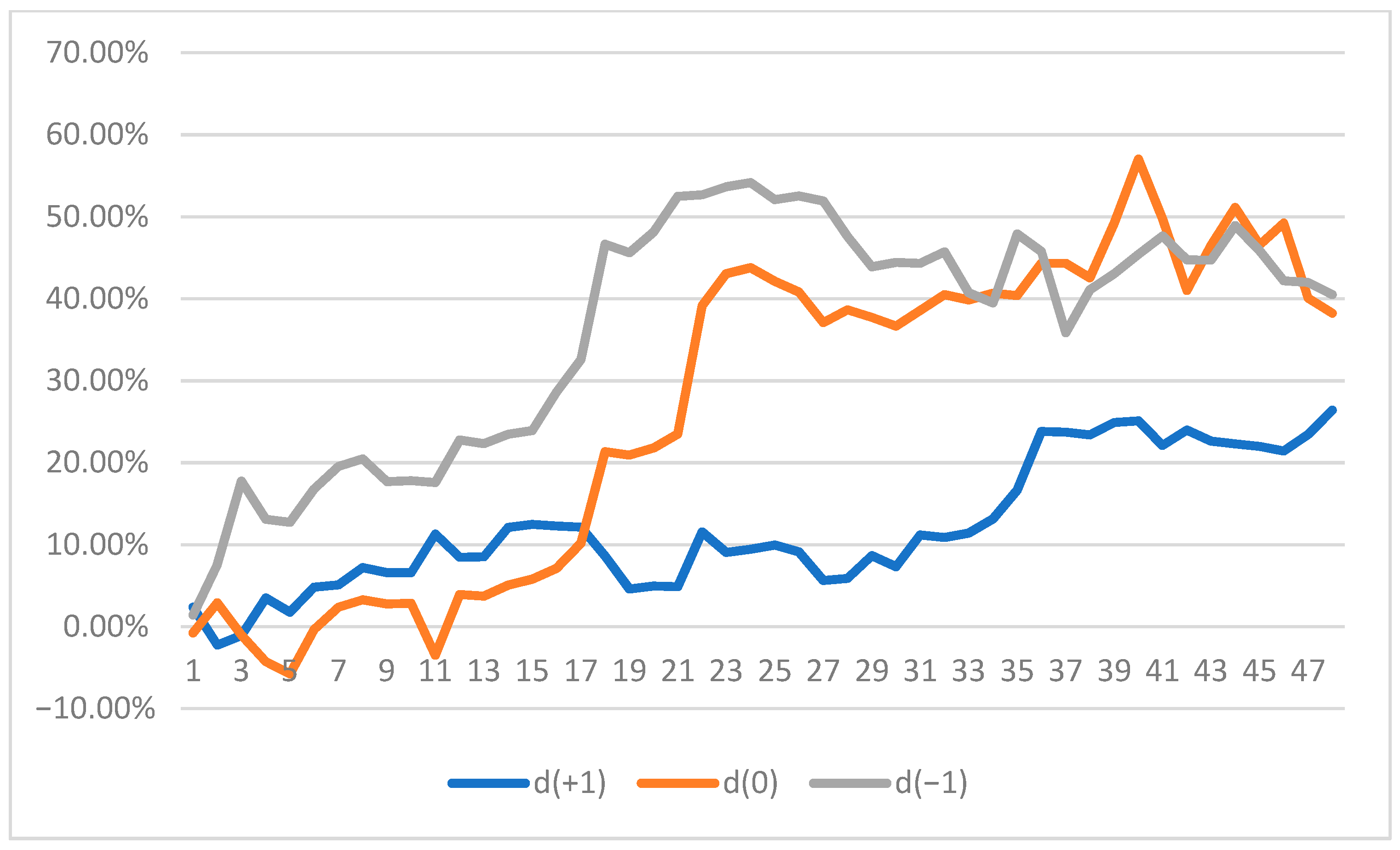
As can be seen, there is strong preliminary evidence in favor of differences in returns between usual days and expiration days (see Table A1 and Figure A1 for details). However, these differences are statistically insignificant.
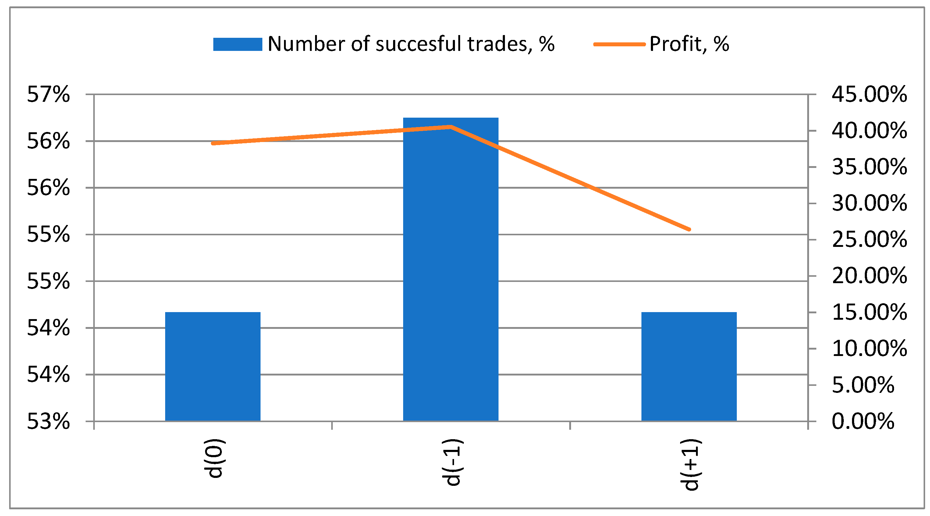
To determine whether the detected effects could allow market participants to “beat the market”, the following trading algorithm was used for d(0): sell right at the start of the witching day. Positions should be closed at the end of the witching day. Additional strategies to be tested on d(−1) and d(+1) were as follows: buy right at the start of the day before and after the expiration day, with further closure of these positions at the end of the day.
The results of the trading simulation are presented in Table 2 and Figure 1 and Figure 2.
The analyzed trading strategies did not provide trading opportunities that were statistically different from random trading. This means that returns on the expiration day and previous/next days did not differ from usual daily returns, and there were no trading opportunities related to witching days or to the days before and after a witching day. These conclusions are confirmed by the Sharpe ratio analysis (all ratios were below 1).

4.2. Weekly Data

Weekly data were analyzed next. The overall results for the usual weeks and witching-related weeks are presented in Table 3.
In most cases, the average analysis showed differences in returns between the usual weeks and the expiration-day related weeks (see Table A7 and Figure A2 for details). However, these differences were statistically insignificant in all cases.
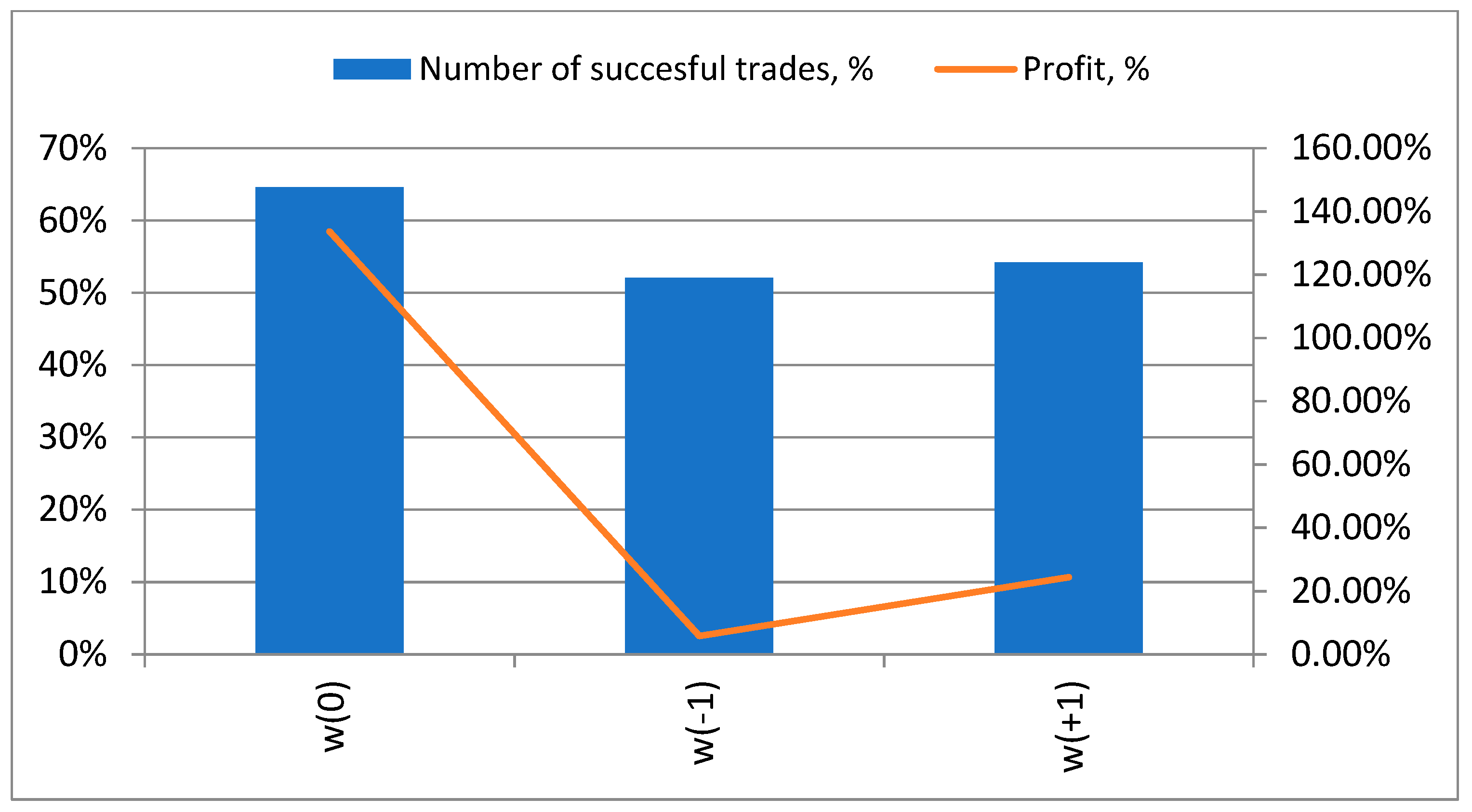
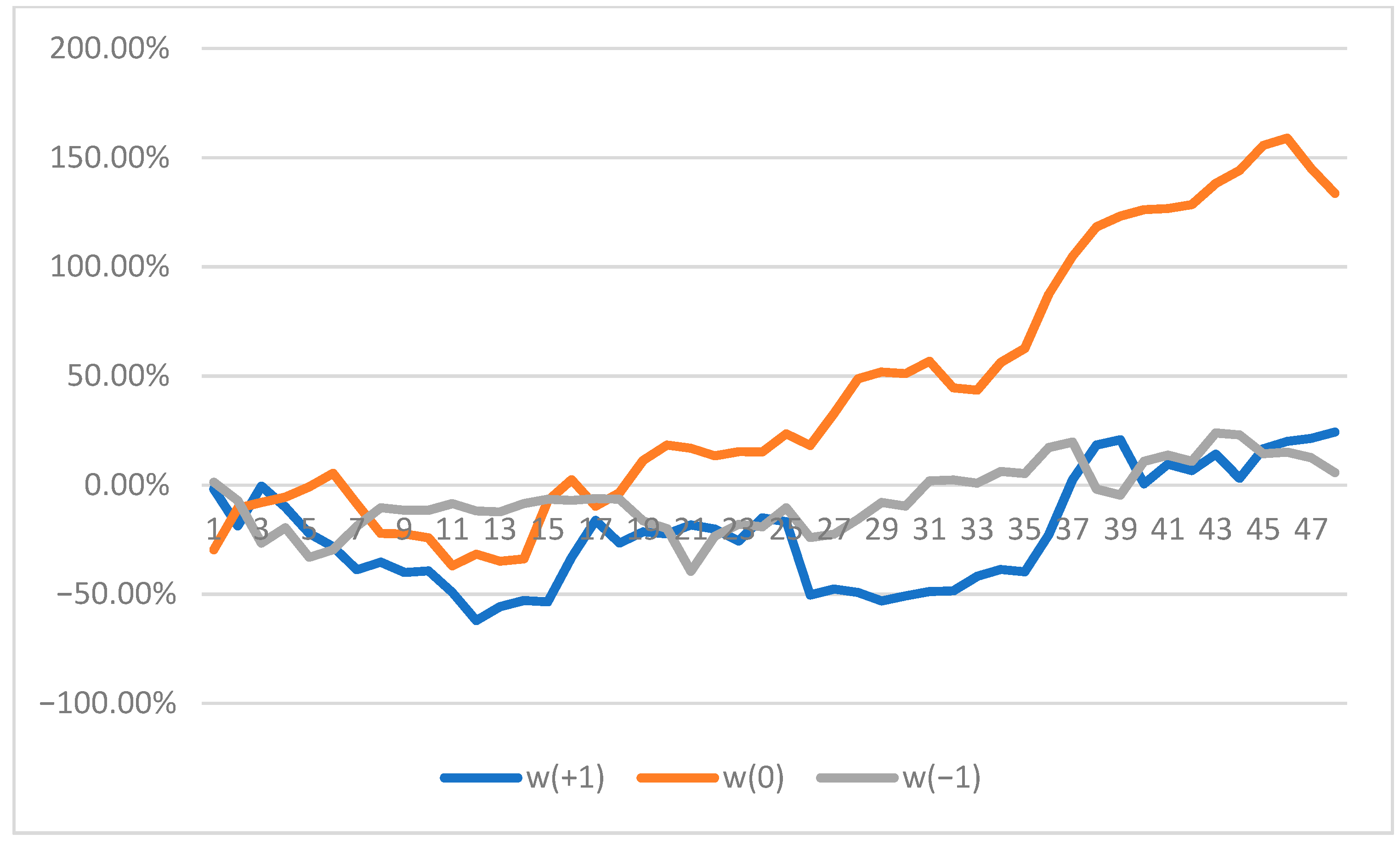
To determine whether this statistical anomaly was able to be exploited to generate abnormal profits from trading, a trading simulation was applied (see Table 4 and Figure 3 and Figure 4 for details). The trading strategy analyzed was as follows: “buy right at the start of the week and close this position at the end of the week”.
As can be seen, trading strategies based on the week before the expiration day w(−1) and the week after the expiration day w(+1) do not demonstrate results in light of these price effects that are different from random trading. Their inefficiency is confirmed by Sharpe ratios below 1. However, during the week including the expiration day, the number of successful trades was 65%, the results of the simulations were different from those of random trading, and Sharpe ratio was above 1.
In conclusion, expiration effects in the cryptocurrency market in most cases are myths. The roots of these myths are quite clear: because of the high volatility of Bitcoin returns and the relatively small data sample, there is an impression that available differences in average returns on expiration days or related periods are much higher/lower than the usual ones. However, these differences are statistically insignificant. As a result, these effects are just illusions, and cannot be exploited in practice. The only exception to this is that returns during an expiration week were more than 5 times greater than the usual ones, and trading strategies based on this fact were able to generate results that were different from random trading, with a Sharpe ratio above 1. This provides evidence in favor of the existence of a real price anomaly.
The detection of an anomaly in the form of abnormally high returns during expiration weeks might be an object of interest for from the practitioners and academics. For academics, this is further evidence contradicting the efficient market hypothesis, and additional evidence in favor of the expiration effect in financial markets. For practitioners (traders, investors, asset managers, etc.), this information could be useful for improving asset management and trading processes. This could be the case for time series forecasting analysis as well: the use of expiration periods as additional variables (for example, as dummy variables) could increase the overall quality of models. Technical analysis methodologies might be improved by developing specific indicators based on the detected effect.
The limitations of this paper include the following aspects. Transaction costs were not incorporated into the trading simulation approach. Despite low transfer fees and spreads, transaction costs remain an important element of trading. In the case of the insignificant advantages obtained using the simulated trading strategies, their actual efficiency when including transaction costs may not differ from random trading. At the current time, the history of expirations is very limited in the cryptocurrency market (only 3 years for the case of Bitcoin).
Future research directions include further objects of analysis, with futures and options being available for other cryptocurrencies as well (there are currently 6000+ cryptocurrencies, but derivatives are only available in the case of Bitcoin). More precise trading simulations could be applied to the developed strategies in order to obtain results that are fully adjusted to real-life scenarios. More sophisticated methodologies could be applied to the most recent data in order to generate reliable results. Additional discussions explaining the results could be provided in future works. The cryptocurrency market is changing quite actively (Giudici and Pagnottoni 2019), and as a result, it will be necessary to revise the presented results. A separate aspect might be the development of technical analysis indicators to generate trading signals based on detected patterns.

5. Conclusions

This paper explores the specific price behavior in the cryptocurrency market related to so-called “witching days” (expiration days of crypto derivatives). Using Bitcoin daily and weekly data over the period 2018–2021, the following hypotheses are tested: (H1) Expiration days create patterns in price behavior in the cryptocurrency market; and (H2) Price patterns can be exploited to generate abnormal profits from trading.
For these purposes, different statistical tests (parametric Student’s t-test, ANOVA, non-parametric Mann–Whitney test) and specific methods (regression analysis with dummy variables, trading simulation approach) were applied to assess the daily and weekly returns in the cases of days/weeks in which an expiration day was present, the day/week before an expiration day and the day/week after an expiration day.
The results suggest the absence of statistically significant price effects related to expiration days in daily returns. Some minor evidence in favor of anomaly were found only in the case of weekly data: in 65% of cases, returns during such weeks were positive, and they were more than 5 times greater than the usual ones. A trading strategy based on this fact could generate results that were different from random ones, providing evidence in favor of real price anomaly.
The presence of abnormally high returns during expiration weeks contradicts the efficient market hypothesis (EMH), and generally appears strange in the context of the 21st century, which is characterized by algorithmic and high-frequency trading, in which the smallest number of trading opportunities tend to be explored. Still, these results provide some evidence in favor of exploitable profit opportunities. These can be used by traders or investors to generate additional returns. Technical analysts could develop a specific indicator to generate trading signals based on detected price patterns. For academics, the results of this paper are interesting not only as additional evidence challenging the EMH, but because they may help improve time series forecasting analysis in the case of Bitcoin by incorporating expiration periods as additional variables in models, improving their overall efficiency.
Future research directions could include additional objects of analysis and data sets, the development of trading strategies based on the revealed effects, the use of more sophisticated methodologies to test the hypotheses explored in this paper, further discussion explaining the detected anomaly, and the development a technical analysis indicator in order to generate trading signals based on the detected patterns.

Author Contributions

Conceptualization, A.P. and L.K.; methodology, A.P.; software, S.B.; validation, A.P., L.K. and S.B.; formal analysis, A.P.; investigation, S.B.; resources, A.P. and L.K.; data curation, A.P.; writing—original draft preparation, A.P., L.K. and S.B.; writing—review and editing, A.P.; visualization, L.K. and S.B.; supervision, A.P.; project administration, A.P.; funding acquisition, A.P. All authors have read and agreed to the published version of the manuscript.

Funding

This research received no external funding.

Institutional Review Board Statement

Not applicable.

Informed Consent Statement

Not applicable.

Data Availability Statement

The data source is Yahoo Finance (https://finance.yahoo.com/). accessed on 5 January 2022.

Acknowledgments

Alex Plastun gratefully acknowledges financial support from the Ministry of Education and Science of Ukraine (0121U100473).

Conflicts of Interest

The authors declare no conflict of interest.

Appendix A

Daily Data

Figure A1. Average returns for the usual days and expiration-related days.
Jrfm 15 00092 g0a1
Table A1. Average returns for the usual days and expiration-related days.
Case of AnalysisUsual DayExpiration-Related DayANOVA Multiplier *
d(0)0.02%−0.22%1.28
d(−1)0.02%0.12%0.20
d(+1)0.02%0.19%0.63
* F/Fcrit from ANOVA analysis ratio, which makes it possible to see how statistically significant the difference is. When this multiplier is above 1, it might be concluded that there is a statistically significant difference between returns.
Table A2. ANOVA test of the expiration day price effects.
Case of AnalysisFp-ValueF CriticalNull HypothesisAnomalyANOVA Multiplier
d(0)1.380.243.85not rejectednot confirmed0.36
d(−1)2.790.093.85not rejectednot confirmed0.73
d(+1)0.580.453.85not rejectednot confirmed0.15
Table A3. Mann–Whitney test of the expiration day price effects.
Case of AnalysisAdjusted Hd.f.p ValueCritical ValueNull HypothesisAnomalyMann–Whitney Multiplier
d(0)0.961.000.333.84not rejectednot confirmed0.25
d(−1)2.381.000.123.84not rejectednot confirmed0.62
d(+1)0.681.000.413.84not rejectednot confirmed0.18
Table A4. T-test of the expiration day price effects.
PeriodParameterUsual DayExpiration-Related DayPeriodUsual DayExpiration-Related DayPeriodUsual DayExpiration-Related Day
d(0)Mean, %0.12%0.78%d(−1)0.12%−0.83%d(+1)0.12%0.54%
Stand. Dev., %3.91%4.61%3.91%4.10%3.91%2.57%
Number of values144248144248144248
t-criterion0.991.571.10
Null hypothesisnot rejectednot rejectednot rejected
Anomalynot confirmednot confirmednot confirmed
Table A5. Modified CAR approach: results of the expiration day price effects *.
Case of AnalysisMultiple RF-Testa0a1Anomaly
d(0)0.90192.73 (0.00)−0.0501 (0.04)0.0117 (0.00)confirmed
d(−1)0.7975.85 (0.00)−0.1756 (0.00)−0.0089 (0.00)confirmed
d(+1)0.7976.46 (0.00)0.0021 (0.86)0.0037 (0.00)confirmed
* p-values are in parentheses.
Table A6. Regression analysis with dummy variables: results of the expiration day price effects *.
Case of AnalysisMultiple RF-Testa0a1Anomaly
d(0)0.031.38 (0.24)0.0012 (0.26)0.0068 (0.24)not confirmed
d(−1)0.042.79 (0.09)0.0012 (0.25)−0.0096 (0.09)not confirmed
d(+1)0.020.58 (0.45)0.0012 (0.25)0.0043 (0.45)not confirmed
* p-values are in parentheses.

Appendix B

Weekly Data

Table A7. Average returns for the usual weeks and expiration-related weeks.
Case of AnalysisUsual WeekExpiration-Related WeekANOVA Multiplier *
w(0)0.50%2.73%0.46
w(−1)0.50%0.12%0.01
w(+1)0.50%0.50%0.00
* F/Fcrit from ANOVA analysis ratio, which makes it possible to see how statistically significant the difference is. When this multiplier is above 1, it might be concluded that there is a statistically significant difference between returns.
Figure A2. Average returns for the usual weeks and expiration-related weeks.
Jrfm 15 00092 g0a2
Table A8. ANOVA test of the expiration price effects.
Case of AnalysisFp-ValueF CriticalNull HypothesisAnomalyANOVA Multiplier
w(0)1.770.183.89not rejectednot confirmed0.46
w(−1)0.050.823.89not rejectednot confirmed0.01
w(+1)0.001.003.89not rejectednot confirmed0.00
Table A9. Mann–Whitney test of the expiration price effects.
Case of AnalysisAdjusted Hd.f.p ValueCritical ValueNull HypothesisAnomalyMann–Whitney Multiplier
w(0)2.591.000.113.84not rejectednot confirmed0.67
w(−1)0.011.000.913.84not rejectednot confirmed0.00
w(+1)0.001.000.993.84not rejectednot confirmed0.00
Table A10. T-test of the expiration price effects.
PeriodParameterUsual WeekExpiration-Related WeekPeriodUsual WeekExpiration-Related WeekPeriodUsual WeekExpiration-Related Week
w(0)Mean, %0.50%2.73%w(−1)0.50%0.12%w(+1)0.50%0.50%
Stand. Dev., %10.35%10.81%10.35%8.53%10.35%10.94%
Number of values166481664816648
t-criterion1.270.260.00
Null hypothesisnot rejectednot rejectednot rejected
Anomalynot confirmednot confirmednot confirmed
Table A11. Modified CAR approach: results of the expiration price effects *.
Case of AnalysisMultiple RF-Testa0a1Anomaly
w(0)0.91224.27 (0.00)−0.5776 (0.00)0.0355 (0.00)confirmed
w(−1)0.325.33 (0.02)−0.2454 (0.00)0.0026 (0.02)confirmed
w(+1)0.242.85 (0.10)−0.4382 (0.00)0.0039 (0.10)not confirmed
* p-values are in parentheses.
Table A12. Regression analysis with dummy variables: results of the expiration price effects *.
Case of AnalysisMultiple RF-Testa0a1Anomaly
w(0)0.091.77 (0.18)0.0050 (0.54)0.0228 (0.18)not confirmed
w(−1)0.020.05 (0.82)0.0050 (0.52)−0.0038 (0.82)not confirmed
w(+1)0.000.00 (0.99)0.0051 (0.53)−0.0001 (0.99)not confirmed
* p-values are in parentheses.

References

  1. Alkebäck, Per, and Niclas Hagelin. 2004. Expiration day effects of index futures and options: Evidence from a market with a long settlement period. Applied Financial Economics 14: 385–96. [Google Scholar] [CrossRef]
  2. Arago, Vicent, and Maria Angekes Fernandez. 2002. Expiration and maturity effect: Empirical evidence from the Spanish spot and futures stock index. Applied Economics 34: 1617–26. [Google Scholar] [CrossRef]
  3. Batrinca, Bogdan, Christian Hesse, and Philip Treleaven. 2020. Expiration day effects on European trading volumes. Empirical Economics 58: 1603–38. [Google Scholar] [CrossRef] [Green Version]
  4. Bollen, Nicolas, and Robert Whaley. 1999. Do expirations of Hang Seng Index derivatives affect stock market volatility? Pacific-Basin Finance Journal 7: 453–70. [Google Scholar] [CrossRef]
  5. Caihong, Xu. 2014. Expiration-Day Effects of Stock and Index Futures and Options in Sweden: The Return of the Witches. Journal of Futures Markets 34: 868–82. [Google Scholar]
  6. Caporale, Guglielmo Maria, and Plastun Alex. 2021. Witching Days and Abnormal Profits in the US Stock Market. CESifo Working Paper No. 9360. Available online: https://ssrn.com/abstract=3950095 (accessed on 16 February 2022).
  7. Chay, Jong Bom, and Han Ryu. 2006. Expiration-day effects of the KOSPI 200 futures and options. Asia-Pacific Journal of Financial Studies 35: 69–101. [Google Scholar]
  8. Chow, Ying-Foon, Hyanes Yung, and Hua Zhang. 2003. Expiration day effects: The case of Hong Kong. Journal of Futures Markets: Futures, Options, and Other Derivative Products 23: 67–86. [Google Scholar] [CrossRef]
  9. Chung, Huimin, and Mei-Maun Hseu. 2008. Expiration day effects of Taiwan index futures: The case of the Singapore and Taiwan Futures Exchanges. Journal of International Financial Markets 18: 107–20. [Google Scholar] [CrossRef]
  10. Corredor, Pilar, Pedro Lechon, and Rafael Santamaria. 2001. Option-expiration effects in small markets: The Spanish stock exchange. Journal of Futures Markets: Futures, Options, and Other Derivative Products 21: 905–28. [Google Scholar] [CrossRef]
  11. Edwards, Franklin. 1988. Does futures trading increase stock market volatility? Financial Analysts Journal 44: 63–69. [Google Scholar] [CrossRef]
  12. Giudici, Paolo, and Paolo Pagnottoni. 2020. Vector error correction models to measure connectedness of Bitcoin exchange markets. Applied Stochastic Models in Business and Industry 36: 95–109. [Google Scholar] [CrossRef] [Green Version]
  13. Giudici, Paolo, and Paolo Pagnottoni. 2019. High Frequency Price Change Spillovers in Bitcoin Markets. Risks 7: 111. [Google Scholar] [CrossRef] [Green Version]
  14. Gurgul, Henryk, and Milena Suliga. 2019. Impact of futures expiration on underlying stocks: Intraday analysis for Warsaw Stock Exchange. Central European Journal of Operations Research 2: 1–36. [Google Scholar] [CrossRef] [Green Version]
  15. Hsieh, Shu-Fan, and Tai Ma. 2009. Expiration-day effects: Does settlement price matter? International Review of Economics & Finance 18: 290–300. [Google Scholar] [CrossRef]
  16. Karolyi, George. 1996. Stock market volatility around expiration days in Japan. Journal of Derivatives 4: 23–43. [Google Scholar] [CrossRef]
  17. MacKinlay, Craig. 1997. Event studies in economics and finance. Journal of Economic Literature 35: 13–39. [Google Scholar]
  18. Mazanec, Jaroslav. 2021. Portfolio Optimalization on Digital Currency Market. Journal of Risk and Financial Management 14: 160. [Google Scholar] [CrossRef]
  19. Pope, Peter, and Pradeep Yadav. 1992. The impact of option expiration on underlying stocks: The UK evidence. Journal of Business Finance and Accounting 19: 329–44. [Google Scholar] [CrossRef]
  20. Resta, Marina, Paolo Pagnottoni, and Maria E. De Giuli. 2020. Technical Analysis on the Bitcoin Market: Trading Opportunities or Investors’ Pitfall? Risks 8: 44. [Google Scholar] [CrossRef]
  21. Schlag, Christian. 1996. Expiration day effects of stock index derivatives in Germany. European Financial Management 2: 69–95. [Google Scholar] [CrossRef]
  22. Singh, Gurmeet, and Muneer Shaik. 2020. Re-examining the Expiration Effects of Index Futures: Evidence from India. International Journal of Economics and Financial Issues 10: 16–23. [Google Scholar] [CrossRef]
  23. Stoll, Hans, and Robert Whaley. 1987. Program trading and expiration-day effects. Financial Analysts Journal 43: 16–28. [Google Scholar] [CrossRef]
  24. Stoll, Hans, and Robert Whaley. 1991. Expiration-day effects: What has changed? Financial Analysts Journal 47: 58–72. [Google Scholar] [CrossRef]
  25. Vipul, Vipul. 2005. Futures and options expiration-day effects: The Indian evidence. Journal of Futures Markets 25: 1045. [Google Scholar]
  26. Yoo, S. 2017. The Expiration Day Effects of Single Stock Futures: Evidence from Korea. Journal of Derivatives and Quantitative Studies 25: 451–78. [Google Scholar] [CrossRef]
Figure 1. Trading simulation results of the expiration day price effects: daily data.
Jrfm 15 00092 g001
Figure 2. Trade by trade profit/loss dynamics: daily data.
Jrfm 15 00092 g002
Figure 3. Trading simulation results of the expiration price effects: weekly data.
Jrfm 15 00092 g003
Figure 4. Trade by trade profit/loss: weekly data.
Jrfm 15 00092 g004
Table 1. Overall results for expiration price effects: the daily data.
Case of AnalysisAverage AnalysisStudents t-TestANOVAMann–Whitney TestModified CARRegression with Dummy
Variables
Trading SimulationOverall
d(0)+---+--2
d(−1)+---+--2
d(+1)+---+--2
Note: This table presents the overall results calculated on the basis of daily data. “+” indicates that an anomaly is confirmed, and “-” indicates that an anomaly is not confirmed. The average analysis confirms an anomaly if the mean return calculated for the expiration-related day is much higher (lower) compared with the mean return calculated for usual-day data. The statistical tests’ (both parametric and non-parametric) rejection of the null hypothesis (data for witching-related days and usual days belong to the same general population) also confirms the presence of an anomaly, if it is statistically significant. The regression analysis with dummy variables provides evidence in favor of the presence of an anomaly if a1 (slope of the dummy variable) is statistically significant (p < 0.05). The MCAR approach confirms the presence of an anomaly if the trend model based on cumulative abnormal returns data has high multiple R, passes the F test, and the regression coefficients are statistically significant (p-value < 0.05). The higher the overall rating, the stronger the evidence for an anomaly.
Table 2. Trading simulation results of the expiration day price effects: daily data.
Case of AnalysisNumber of Trades, UnitsNumber of Successful Trades, UnitsNumber of Successful Trades, %Profit, %Profit % per Tradet-Test Calculated Valuet-Test StatusSharpe Ratio
d(0) *482654%38.25%0.80%1.20failed0.40
d(−1) **482756%40.51%0.84%1.43failed0.50
d(+1) *482654%26.41%0.55%1.49failed0.25
* positive returns; ** negative returns.
Table 3. Overall results for the expiration price effects: weekly data.
Case of AnalysisAverage AnalysisStudents t-TestANOVAMann–Whitney TestModified CARRegression with Dummy
Variables
Trading SimulationOverall
w(0)+---+-+3
w(−1)+---+--2
w(+1)-------1
Note: This table presents the overall results calculated on the basis of the weekly data. “+” indicates that the presence of an anomaly is confirmed, and “-” indicates that the presence of an anomaly is not confirmed. The average analysis confirms the presence of an anomaly if the mean return calculated for the witching-related week is much higher (lower) compared with the mean return calculated for a usual week. The statistical tests’ (both parametric and non-parametric) rejection of the null hypothesis (data for witching-related weeks and normal weeks belong to the same general population) also confirms the presence of an anomaly if it is statistically significant. The regression analysis with dummy variables provides evidence in favor of the presence of an anomaly if a1 (slope of the dummy variable) is statistically significant (p < 0.05). The MCAR approach confirms the presence of an anomaly if the trend model based on cumulative abnormal returns data has high multiple R, passes the F test, and the regression coefficients are statistically significant (p-value < 0.05). The higher the overall rating, the stronger the evidence for an anomaly.
Table 4. Trading simulation results for expiration price effects: weekly data.
Case of AnalysisNumber of Trades, UnitsNumber of Successful Trades, UnitNumber of Successful Trades, %Profit, %Profit % per Tradet-Test Calculated Valuet-Test StatusSharpe Ratio
w(0) *483165%133.67%2.78%1.79passed1.05
w(−1) *482552%5.81%0.12%0.10failed−0.17
w(+1) *482654%24.36%0.51%0.32failed0.04
* positive returns.
Publisher’s Note: MDPI stays neutral with regard to jurisdictional claims in published maps and institutional affiliations.

