Abstract
A data envelopment analysis (DEA) has yet to be chosen to assess countries’ financial inclusion levels. We introduce an application of the DEA methodology to compute aggregate performance measures regarding the financial inclusion of economies. We specifically explore composite scores based on relative efficiency, super-efficiency, and cross-efficiency approaches. We implement the proposed procedure to study the financial inclusion in nations from the West African Economic and Monetary Union (WAEMU). We use the Union’s Central Bank’s financial inclusion data from 2010 to 2017. We obtain robust financial inclusion level measures, showing that overall, in the Union, there have been steady improvements during the study period, but with heterogenous behavior at the level of each economy. A benchmarking analysis allowed us to determine the countries with the best practices. For the remaining nations, we find their reference countries. Finally, we identified which financial service sectors drive the financial inclusion in each country from the optimal weights of the DEA model.
1. Introduction
Financial inclusion has recently been a significant concern for the international community. This is particularly true for developing countries, especially in sub-Saharan Africa. In 2021, according to the latest Global Findex survey of The World Bank (Demirgüç-Kunt et al. 2022), a proportion of 76% of adults at the global level possessed an account at a bank or a regulated institution such as a credit union, a microfinance institution, or a mobile money service provider. At the global level, this rate has improved by 50% since the first such survey in 2011 (Demirgüç-Kunt and Klapper 2012). However, when one considers sub-Saharan African countries, this proportion of adults owning an account drops to 55% (Demirgüç-Kunt et al. 2022). Hence, financial exclusion is a particularly acute problem in many African countries. Indeed, the banking systems in these countries are deemed less inclusive (Zins and Weill 2016). However, there is an interesting fact worth noting. Despite exhibiting a relatively low rate of adults owning an account at a bank or a regulated institution, sub-Saharan Africa had the most significant proportion of adults retaining an account at a mobile money service provider at 33% (Demirgüç-Kunt et al. 2022).
Financial inclusion is a multidimensional concept. According to several scholars and international organizations, such as the Alliance for Financial Inclusion (AFI) and the Central Bank of West African States (BCEAO), financial inclusion is defined following all, or part of, the following prisms or dimensions: access, quality, usage, and well-being. It can be determined from a production economics perspective. It is then expected to result in an improvement of economic productivity (AFI 2010; Arun and Kamath 2015; BCEAO 2018a, 2018b; Demirgüç-Kunt et al. 2015; Le et al. 2019; Pearce and Ortega 2012; Zins and Weill 2016). The concept of financial inclusion can also be outlined through the lens of development economics as one of the tools that can help alleviate poverty (Arun and Kamath 2015).
Due to its complex (multidimensional) nature, it is particularly challenging to evaluate financial inclusion. Specifically, providing a quantified answer to questions about what the financial inclusion level of a country or an economy is, or should be, requires significant work. Originally, the financial inclusion status was assessed using a single surrogate indicator. Such an indicator is, for example, the rate of adults at the global level owning an account at a bank or at a regulated institution such as a credit union, a microfinance institution, or a mobile money service provider, used by Demirgüç-Kunt et al. (2022). This index was initially proposed as the proportion of adults having an account in a formal financial institution (bank, credit union, microfinance institution) in the first Global Findex survey (Demirgüç-Kunt and Klapper 2012; Guérineau and Jacolin 2014). It was later revised to integrate mobile money services (Demirgüç-Kunt et al. 2015, 2018, 2022).
With a single indicator, only partial information is involved in the assessment of financial inclusion. This is a major inconvenience with the previous approach. To correct this shortcoming, several authors proposed to aggregate several indices into a composite index (Becker et al. 2017; Foster et al. 2013; Greco et al. 2019; Nardo et al. 2005). With such an aggregate measure, the performance of entities is better evaluated. Indeed, one obtains a summary numerical measure which incorporates multiple criteria or attributes, combined using weight. These weights illustrate the relative importance of each attribute (Permanyer 2011). Composite indicators (also known as synthetic indices or performance indices) are popular instruments due to their simplicity. They have been adopted to study several concepts such as human development, sustainability, perceived corruption, innovation, competitiveness, entrepreneurship, and corporate social responsibility (Ahamed and Mallick 2019; Anarfo et al. 2020; Cámara and Tuesta 2014; Cherchye 2001; Cherchye and Kuosmanen 2004; Cherchye et al. 2004; Greyling and Tregenna 2017; Lovell et al. 1995; Mahlberg and Obersteiner 2001; Melyn and Moesen 1991; Nicoletti et al. 2000; Storrie and Bjurek 2000; Takouda et al. 2022). Nevertheless, the use of synthetic indices is not exempt from criticism. According to some scholars and practitioners, such instruments are statistically meaningless (Greco et al. 2019).
Composite indices measuring financial inclusion levels have been proposed in the literature. Sarma (2008, 2012) proposed measures calculated using the technique of order preference similarity to the ideal solution (TOPSIS) (Behzadian et al. 2012; Chakraborty 2022). Most approaches used to calculate composite measures of financial inclusion were based on principal component analysis (PCA), a multivariate statistical technique (Greco et al. 2019; Nardo et al. 2005). The PCA’s goal is to capture the largest variance possible in the original (standardized) variables within as few components as possible. When one constructs composite indicators, the PCA provides a data-driven approach. Actual data drive the selection of aggregation weights, as opposed to them being chosen subjectively or assumed to be all equal (Ahamed and Mallick 2019; Anarfo et al. 2020; Cámara and Tuesta 2014; Greyling and Tregenna 2017; Nicoletti et al. 2000). It is worth noting, however, that other important decisions, such as how many principal components shall be considered and retained, and whether a rotation method shall be used, may be made subjectively. We usually have rules of thumb to help make such choices (Nicoletti et al. 2000).
Cámara and Tuesta (2014) used data from Demirgüç-Kunt and Klapper (2012) to determine financial inclusion status aggregate measures. They considered three dimensions: usage, access, and barriers to access and used a two-step PCA approach. First, composite scores of each dimension are computed; then, these dimensional measures are aggregated to determine the overall measure. PCA was the aggregation tool in each case, and all principal components were incorporated into the measure. Ahamed and Mallick (2019) used a similar two-step PCA approach on data from the Financial Access Survey (FAS) from the International Monetary Fund (IMF) for a sample of 3635 banks from 86 countries between 2004 and 2012. There were two slight differences. Only two dimensions (access and usage) are considered, and the dimensional scores, in the first step, were based on the first principal component. Anarfo et al. (2020), on the other hand, used a classical PCA approach to find composite scores from six (6) indicators for a sample of 217 countries, including 48 sub-Saharan economies, for the period 1990–2014.
From the composite indices’ construction literature (Greco et al. 2019; Nardo et al. 2005), besides PCA, data envelopment analysis (DEA) is the other data-driven approach that is frequently used. DEA is a non-parametric methodology used to measure the relative efficiency of a collection of decision-making units (DMUs) considering several inputs and outputs (Charnes et al. 1978). It has been used extensively in recent decades, with applications to measure the performance or relative efficiency of private and public organizations’ multiple sectors, including retail (Takouda and Dia 2016, 2019), mining, and oil and gas production (Dia et al. 2019, 2021), as well as financial services (Dia et al. 2020a, 2020b). Recent surveys of DEA applications can be found in the work of Chen et al. (2019), Emrouznejad and Yang (2018), and Fosso Wamba et al. (2018).
To build aggregate measures using DEA, one must use the benefit of the doubt (BoD) approach (Greco et al. 2019; Nardo et al. 2005; Ouattara et al. 2021; Takouda et al. 2020; Takouda et al. 2022). Such technique considers only one input, set equal to one (1), and all the indicators that must be aggregated as outputs. BoD has been applied to assess performance of various concepts, such as macroeconomic policies, labor market, social inclusion, entrepreneurship, and corporate social responsibility (Aparicio and Kapelko 2019; Cherchye 2001; Cherchye and Kuosmanen 2004; Cherchye et al. 2004; Lovell et al. 1995; Mahlberg and Obersteiner 2001; Melyn and Moesen 1991; Ouattara et al. 2021; Storrie and Bjurek 2000; Takouda et al. 2020; Takouda et al. 2022). Unlike PCA, DEA does not require the existence of a correlation between indicators. Furthermore, with DEA, we obtain weights sensitive to each government’s political priorities. This is good since we are assessing countries’ strategies or policies. It also eliminates suspicions of bias in the selection of the weights since the weights applied to each country are the best, comparatively to the other countries in the sample. Finally, with DEA, we can perform a benchmarking analysis.
Despite its popularity and wide range of applications, the DEA methodology has seldom been used to build composite financial inclusion measures. We are only aware of one application we proposed in the work of Takouda et al. (2020). A possible explanation for this situation may be some limitations that the DEA has. First, we may obtain optimal sets of weights that are not realistic. This results from optimizing while considering all possible combinations of weights. We can avoid this issue with the imposition of restrictions on the ranges of values that the weights can assume. This approach is called DEA with weight restrictions (Greco et al. 2019). DEA can also suffer from a lack of discrimination power among the units. This happens for example with DMUs considered efficient, who all have the same optimal score equal to one (1). Hence, if we want to rank DMUs, we cannot differentiate among efficient units. With post hoc DEA models, such as super-efficiency and cross-efficiency DEA models (Alvarez et al. 2020; Angulo-Meza and Lins 2002; Doyle and Green 1994; Greco et al. 2019), this other problem can be fixed. Finally, especially with data coming from surveys, there is a risk of uncertainty or lack of accuracy of the data. When using DEA models, bootstrapping (Simar and Wilson 1998, 2000; Toma et al. 2017) can mitigate the impact of these problems.
In summary, the data envelopment analysis (DEA) methodology can be applied to build composite measures of countries’ financial inclusion levels. However, it has rarely been performed in the literature. We intend to contribute to closing this gap, and to use the DEA methodology to evaluate the financial inclusion status of the economies in the West African Economic and Monetary Union (WAEMU) from 2010 to 2017. WAEMU is an economic region with unique characteristics, which makes it interesting to analyze. First, from the economic history point of view, seven of the eight countries of the union were French colonies. Hence, the creation of the union in January 1994 coincided with the devaluation of the CFA Franc, the common currency of those previous French colonies. The union’s objective was to enable economic integration based on a common market, competitive economies, and a convergence of the performances of the political and economic institutions. WAEMU is also an economic zone distinguished by atomistic markets, exhibiting a recent and exponential growth of the offer of mobile money services, followed by a significative development of financial service firms which integrate innovations from the information and communication technologies (fintech) in their activities.
We can summarize our contribution in this paper as follows. We extend the work presented by Takouda et al. (2020) by applying the post hoc DEA models to calculate aggregate measures of the financial inclusion level, allowing for a better discrimination between countries. More specifically, we compute composite financial inclusion scores in WAEMU using the classic DEA, the super efficiency DEA, as well as the benevolent and the aggressive cross-efficiency DEA models. We compare these scores among each other and with a PCA-based score (Indice Synthétique d’Inclusion Financière (ISIF)), inspired by the approach of Cámara and Tuesta (2014)) published by the Central Bank of West African Countries (BCEAO 2018a, 2018b). The proposed measures are then used to rank the countries according to their levels of financial inclusion. Finally, we perform a benchmarking analysis of the countries and an analysis of the optimal weights of the Charnes–Cooper–Rhodes (CCR) DEA model (Charnes et al. 1978) to identify, for each country, which indicators are the most important or relevant to their levels of financial inclusion.
The rest of the paper is organized as follows. In Section 2, we review the literature on the measurement of financial inclusion levels. The DEA methodology, the benefit of the doubt approach and the post hoc DEA models relevant to the paper are presented in Section 3. Our case study is illustrated in Section 4 and analyzed in Section 5. Section 6 concludes our paper.
2. Measurement of Financial Inclusion Levels: A Literature Review
Financial inclusion (FI) is a multidimensional concept. Each of its dimensions is typically assessed using one of several indicators. Therefore, when one aims to measure overall financial inclusion levels, multicriteria decision-making tools appear as the most appropriate to achieve such an endeavor. There is a diversity of such tools (Doumpos and Zopounidis 2014). In the context of FI, the methodologies used to assess can be seen as based on the utility theory (Doumpos and Zopounidis 2014). In the first of those evaluations, the utility function was derived from only one of the indicators of the dimensions, accepted as the most representative (Demirgüç-Kunt and Klapper 2012; Guérineau and Jacolin 2014; Demirgüç-Kunt et al. 2015, 2018, 2022).
Demirgüç-Kunt and Klapper (2012) were the first to attempt to assess the overall financial inclusion of countries, considering its various dimensions. They used data from the first Global Findex survey, which contained a sample of more than 150,000 adults (15 years or older) selected from 149 countries in 2011. The corresponding database included sixty (60) indicators organized into four categories: account penetration, formal savings, origination of new formal loans, and self-reported barriers to the use of a formal account. The utility function adopted to represent financial inclusion in the study was the percentage of adults owning an account in a formal institution. Demirgüç-Kunt and Klapper (2012) observed that globally, only half of the adults held a bank account, with a heterogeneous statistical distribution across the various regions of the world. For example, the ratio of adults who possess a bank account is weaker in the Middle East and northern Africa (18%), while it reaches 24% in sub-Saharan Africa. Some countries have a high proportion (such as 99% for Denmark), while others exhibit really low ones (such as 2% for Niger, Democratic Republic of Congo, Guinea, or Cambodia).
Moreover, the penetration rate of financial services in the world economies can be explained by their national Gross Domestic Product (GDP), gender, age distribution, education level, and living environment (urban vs. rural). Finally, regarding specifically the WAEMU (considering only Togo, Senegal, Niger, Mali, Guinea-Bissau, Burkina Faso, and Benin), on average, the proportion of adults owning a bank account is 8.26%. It is lower for women (7.28%) than men (9.24%).
Using the same data from the 2017 Global Findex survey, Guérineau and Jacolin (2014) analyzed levels and determinants of financial inclusion in sub-Saharan Africa. They observed that among the economies of that region, those from the Franc zone show a proportion of adults owning a bank account much lower than those from the other emerging and developing countries. They also identify several determinants of access to financial services, which include the level of economic development, the density of banking infrastructures, the quality of transportation services, the cost of financial services (which themselves are impacted by the banking market (concentration and competition)), the asymmetry of information (due to poor perceived quality of financial documentation), age, income, education level, as well as other financial economic and institutional factors.
The Global Findex survey was updated in 2014 (Demirgüç-Kunt et al. 2015) into a database containing a sample of more than 150,000 adults (15 years or older) selected from 143 countries. The database now includes new indicators related to electronic money and domestic payments. There are hence more than a hundred (100) indicators organized into four categories: account penetration, payment means, savings, loans/credits, and financial resilience. The following new observations were made. Globally, a proportion of 2% of adults own a mobile money account. In sub-Saharan Africa, 6% of adults own both a formal bank account and a mobile money one, while another 6% own only a mobile money account. A total of 10% of all adults in sub-Saharan countries owning mobile money accounts lived in five (5) countries: Ivory Coast, Somalia, Tanzania, Uganda, and Zimbabwe. Specifically, in WAEMU, on average, 17% of adults owned a formal account, among whom 7% also owned a mobile money account. Finally, two-thirds of the 143 economies surveyed promoted financial inclusion through various national and regional strategies. However, despite improving overall levels, women and low-income adults still faced financial exclusion.
A second update of the Global Findex survey took place in 2017 (Demirgüç-Kunt et al. 2018), with the same sample size, but this time in 140 economies. It was observed that globally, the proportion of adults owning an account had increased to 69%, with a ratio of 94% for developed countries versus 63% for developing ones. This proportion reduces to 37% on average when only the WAEMU is considered, with 25% also owning a mobile money account. However, the ratio for women (65%) is still lower than for men (72%).
The latest update, the fourth of the Global Findex, occurred in 2021, with a year delay due to the COVID-19 pandemic (Demirgüç-Kunt et al. 2022). The sample was, this time, 128,000 adults in 123 countries, representing 91% of the world population. The survey indicated that the proportion of adults at the global level who possessed an account at a bank or a regulated institution such as a credit union, a microfinance institution, or a mobile money service provider was 76%. The proportion diminishes to 71% for developing countries and 55% for sub-Saharan countries. Interestingly, on the other hand, sub-Saharan countries exhibited the highest proportion of adults who retained an account with a mobile money service provider at 33%. Hence, mobile money service providers seem to be one of the drivers of financial inclusion in these countries. Finally, the gender gap had decreased: it was now 6%.
Some studies (Ahamed and Mallick 2019; Anarfo et al. 2020; Cámara and Tuesta 2014; Sarma 2008, 2012) in the literature used utility functions derived from multiple indicators to assess levels of financial inclusion. Such methodological approaches aim at constructing composite or aggregate indices by aggregating various dimension indicators into a unique transversal index whose value indicates a country’s overall level of financial inclusion. In such an approach, two operations are essential to obtain a high-quality index (Greco et al. 2019; Nardo et al. 2005). First, one must ensure that the indicators are comparable, typically achieved by appropriate scaling. Second, one must determine the value of the aggregation weights, which usually represent each indicator’s relative importance.
Sarma (2008) applied TOPSIS (Behzadian et al. 2012; Chakraborty 2022) to construct two indices to measure each country’s financial inclusion level from a sample based on a given number of dimensions of FI. The first index considers a selection of 55 countries with three dimensions: bank penetration, availability, and use of financial services, while for the second one, only two dimensions (availability and use of financial services) are considered for a sample of now 100 countries. In both cases, each country is represented by a point in three (or two) dimensional space, and the index is calculated as the inverse of the normalized Euclidian distance between the point representing the country and the ideal point (the coordinates of which are all one (1)). Using these indices, countries are ranked, and the orders are not the same for both indices. In Sarma (2012), the same author proposes an alternative method where both the inverses of the distances to the ideal points and to the anti-ideal point (the coordinates of which are all zero (0)) are computed, and the index is calculated as the arithmetic average of these two inverses.
Ahamed and Mallick (2019), Anarfo et al. (2020), and Cámara and Tuesta (2014) use methodologies based on the principal component analysis (PCA), as described by Nardo et al. (2005) and Greco et al. (2019), to build composite indices to measure financial inclusion. Note that when PCA is applied, the analyst can use only the first principal component, a few first principal components, or all of them to compute the index. One-step and two-step procedures have been proposed. In the former, all indicators, regardless of their dimensions, are considered and aggregated. In the latter, in the first step, only indicators related to the same dimension are aggregated, and dimensional indices are obtained. Then, in the second step, dimensional indices are aggregated, again using PCA, to obtain the overall composite index. Compared to the one-step approach, the two-step one is used to minimize the bias of the PCA methods toward strongly correlated indicators.
Cámara and Tuesta (2014) used a two-step PCA approach to compute aggregated indices of financial inclusion using data from the 2011 Global Findex across the three dimensions of use, accessibility, and self-reported barriers (Demirgüç-Kunt and Klapper 2012). In both steps, all the principal components were used to calculate the dimensional indices and the overall ones. The computed comprehensive indices are used to rank countries, provide policy recommendations, and test various hypotheses regarding the relationship between financial inclusion and various variables. Hence, the authors observed correlations between financial inclusion and economic and institutional variables such as the GDP, the education level, the banking system’s efficiency, and the financial system’s development and stability.
Ahamed and Mallick (2019) used supply-side global banks data from the Financial Access Survey (FAS) of the International Monetary Fund (IMF) for the period 2004–2012 to measure levels of inclusion of 86 countries. Indicators of the access and usage dimensions were considered. A two-step PCA approach is also used here. However, for the first step, the dimensional indices are determined using only the first principal component. The computed indices are used to rank countries and test various hypotheses regarding the relationship between financial inclusion and two variables: the stability of the financial system and the quality of the institutions.
Anarfo et al. (2020) used supply-side global banks data from the International Financial Statistics (IFSs) for the period 1990–2014 to measure the financial inclusion status of 217 countries from several continents, including 48 from Africa. They applied a one-step PCA approach to the above data to compute the financial inclusion levels of these 217 economies. Using these results, the authors tested hypotheses on the relationships between financial inclusion and the stability and regulations of the financial system.
In summary, two methodological avenues exist in the literature related to measuring the level of financial inclusion using indicators of the relevant dimensions of the concept. One uses a single indicator, typically the percentage of adults owning an account, considered representative, as the measure. This approach has the limitation of only looking at the access side of financial inclusion and ignoring all the other aspects or dimensions. The second methodological path aggregates several indicators, covering more than one dimension, to derive more composite or transversal measures. This includes approaches where the aggregation’s weights are not explicitly derived, as in the work of Sarma (2008, 2012). When the weights are explicitly determined, the chosen approach is usually PCA. Hence, the approach inherits the limitations of the PCA, mainly the need for strong correlations between indicators to obtain suitable quality measures. In both cases, the measures allow for the ranking of the economies and hypothesis testing. Thankfully, other tools can be used instead of PCA to achieve similar objectives (data-driven composite measures, ranking, hypothesis testing) without the need for strong correlation among indicators.
Such an approach has already been successfully used to compute aggregate measures for multidimensional concepts. It is called the benefit-of-the-doubt (BoD) approach and it uses data envelopment analysis (DEA) as a tool. Using this tool also allows for a benchmarking analysis; hence, an opportunity to identify countries that present the best practices regarding financial inclusion. At the same time, for the remaining countries, target countries that they should emulate to improve their performance are identified as well. Our survey of the literature clearly indicates that the use of the BoD approach has never been reported in the financial inclusion scholarly literature, except for in a conference paper we published previously (Takouda et al. 2020). We intend to contribute to closing that gap with this paper.
3. Data Envelopment Analysis (DEA)
3.1. Basic DEA Models
DEA has been a widely used decision-making technique in recent decades. It is an operational research tool used to assess technical efficiency (Assaf et al. 2011; Daraio and Simar 2007). DEA has hence been applied in multiple industries and sectors, such as agriculture, banking, supply chain management, public policy, etc. We refer the reader interested in the details of these applications to Emrouznejad and Yang (2018), an up-to-date, state-of-the-art, contemporary special issue related to DEA and data analytics (Chen et al. 2019; Fosso Wamba et al. 2018), and specifically for the financial services industry, to the recent book by Paradi et al. (2018).
DEA models assess measure technical efficiencies of decision-making units (DMUs) as a whole. They use the multiple inputs and outputs of the DMUs to determine comprehensive measure of relative efficiency for a sample of DMUs. In addition, with the obtained results, a benchmarking analysis can be performed: efficient units, which represent the best practices are identified, together with reference or target efficient units that the non-efficient ones should emulate to improve their efficiencies. This illustrates the significant benefits of DEA models over parametric models used to assess efficiencies (Banker et al. 1986).
The Charnes–Cooper–Rhodes (CCR) (Charnes et al. 1978) and Banker–Charnes–Cooper (BCC) (Banker et al. 1984) DEA models are the most frequently used. The former assesses overall technical efficiencies, and the latter measures managerial efficiencies. Scale efficiencies are obtained from the ratio of overall technical efficiencies to managerial efficiencies (Banker et al. 1984). We will focus here on introducing the CCR DEA model that we intend to use in our study.
If one denotes by n the number of DMUs, t the number of outputs, m the number of inputs, xis the value of the input s for the DMUi, yir the value of the output r for the DMUi‘s overall technical efficiency score, the DMUi is computed by solving the linear program (LP):
Generally, index i indicates the DMU being assessed, μr is the relative importance of the output r, νs is the relative importance of the input s, and ε is a small positive real number.
For the CCR model (1)–(4), a DMU is efficient if the corresponding optimal ratio hCCR is equal to one (100%). It is inefficient when this ratio is smaller than one. In this model, the ratio can be interpreted as the proportion of the current inputs of the DMU that should yield the current outputs if the DMU were efficient. In other words, the inputs must be reduced by (1 − hCCR) with the same output level if the DMU wants to become efficient.
3.2. Benefit of the Doubt
The benefit of the doubt (BoD) technique consist in using the model (1)–(4) above to compute composite indices (Cherchye 2001; Greco et al. 2019; Nardo et al. 2005; Ouattara et al. 2021; Takouda et al. 2020, 2022). We consider as the outputs the indicators intended to be aggregated and only one input equal to one (1) for all DMUs.
Model (1)–(4) becomes:
Note that with a single input equal to 1, from constraint (2) and in constraint (3).
Here, using DEA, one aims to optimize over all possible combinations of weights to obtain the most favorable composite score for the assessed unit. When our units are countries, the set of optimal weights obtained from model (5)–(8) are sensitive to the political priorities of each country and the composite score calculated is the most favorable for the assessed country (Cherchye 2001; Nardo et al. 2005).
The BoD approach has been applied in several contexts (see Aparicio and Kapelko 2019; Cherchye 2001; Cherchye and Kuosmanen 2004; Cherchye et al. 2004; Lovell et al. 1995; Mahlberg and Obersteiner 2001; Melyn and Moesen 1991; Ouattara et al. 2021; Storrie and Bjurek 2000; Takouda et al. 2020, 2022). We refer the reader to the work of Greco et al. 2019 for a recent detailed review of these applications.
3.3. Post Hoc DEA Models
The DEA methodology has several limitations.
DEA optimizes (see model (1)–(4)) while considering all possible values of the weights (). Some obtained optimal weights may be impractical, in particular in the BoD approach. We consider constraint (7) here, and whether a given weight significantly differs from . It may occur that there is only one weight significantly different from (assigned to the indicator with the highest value), and the weights of all the remaining indicators are not significantly different from . This issue can be fixed by introducing constraints to prevent the weights from assuming certain values. We obtain a model called DEA with weight restrictions. There are multiple possibilities for such restriction constraints, such as direct weight restrictions, cone ratio restrictions, assurance region restrictions, and virtual inputs and output restrictions (see Angulo-Meza and Lins (2002) and Greco et al. (2019)).
Another challenge of DEA is that the efficiency scores may fail to differentiate between some units, for example, when units are efficient. In that case, the score of all (efficient) units is 100%. This is particularly challenging in a BoD approach. A solution to avoid this issue is to use the super-efficiency DEA model (Alvarez et al. 2020; Angulo-Meza and Lins 2002; Greco et al. 2019). We modify constraint (3) in the model (1)–(4), by requiring it to be satisfied for all DMUs except the one (DMUi) being assessed. We obtain the model (8)–(11) below (Alvarez et al. 2020; Angulo-Meza and Lins 2002).
Hence, if DMUi was not efficient previously (), its super-efficiency score obtained from (8)–(11) is the same as the CCR efficiency score from (1)–(4). If the DMU was efficient previously (), its super-efficiency score obtained from (8)–(11), since it is no longer restricted, can be greater than or equal to 100%. Moreover, there is no longer a lack of discrimination issues due to all the efficient units having a score of 100%. A BoD mathematical formulation can be derived similarly as we did for the model (5)–(7).
The cross-efficiencies of units provide an alternative way to increase discrimination among efficient DMUs (Alvarez et al. 2020; Angulo-Meza and Lins 2002; Doyle and Green 1994). The idea is the following. Through the DEA model (1)–(4), the unit being assessed (DMUi) performs a self-evaluation against the other units , and that self-evaluation is derived using the optimal weight . We can then calculate the following quantity:
The quantity is denoted by the cross-efficiency of DMUj using the weighting scheme of DMUi. Therefore, the quantity is precisely the optimal solution from the model (1)–(4). Let us recall that from constraint (2) and .
The cross-efficiencies of DMUj using the weighting scheme of DMUi form a matrix . From the cross-efficiency score of the DMUi is determined as the average of the quantities along the row i, or in other words, the average of all cross-efficiencies calculated using the optimal weighting scheme of DMUi. It is also possible to calculate the average of all the quantities , excluding . Note that all the quantities along the row i are less than or equal to . Hence, the cross-efficiency score of the DMU i is smaller than its self-efficiency .
In practice, the optimal weight obtained from the model (1)–(4) is often not unique. As a result, we may obtain different values for the cross-efficiency score of the DMUi for the same set of DMUs. To fix this issue, secondary goals have to be considered when one calculates these cross-efficiency scores of a DMU (Alvarez et al. 2020; Angulo-Meza and Lins 2002). The most common approaches use benevolent (respectively aggressive) models, which consist in maximizing (respectively minimizing) the sum of all cross-efficiencies of DMUj using the weighting scheme of DMUi, subject to two constraints:
- (a)
- The cross-efficiency of DMUi using the weighting scheme of DMUi remains equal to the optimal solution from the model (1)–(4);
- (b)
- No cross-efficiency of DMUj using the weighting scheme of DMUi is greater than one.
As described above, both benevolent and aggressive models result in nonlinear optimization problems since their objective functions are the sums of ratio functions. It can, however, be linearized into the following linear program for the benevolent approach (Alvarez et al. 2020; Angulo-Meza and Lins 2002).
The quantity is the benevolent cross-efficiency score for DMUi. The linear program corresponding to the aggressive approach is the minimization of the objective function in (12) subjected to the constraints (13)–(16). Again, BoD mathematical formulations can be derived similarly as we did for the models (5)–(7).
4. Case Study
The West African Economic and Monetary Union (WAEMU) (in French, Union Économique et Monétaire Ouest-Africaine (UEMOA)) is an economic zone formed by eight countries: Benin (BE), Burkina Faso (BF), Côte d’Ivoire (CI), Guinée-Bissau (GB), Mali (MA), Niger (NG), Sénégal (SE), and Togo (TG), which are working together toward greater regional integration with unified tariffs. Except for Guinée-Bissau, previously colonized by Portugal, all the above countries were French colonies. All these countries are classified as low or low–middle income countries. They share a central bank, the Central Bank of West African States (BCEAO), which drives the union’s monetary policy. Overall, the financial sector in the WAEMU countries is significantly underdeveloped, with banks dominating the financial sector.
In this context, the central bank, BCEAO, defined inclusive finance as the state in which the population permanently accesses a broad and diversified range of convenient financial services and products at affordable costs, used effectively and efficiently. To monitor and assess the level of financial inclusion, the bank has retained three of the four dimensions adopted in AFI (2010): access, usage, and quality. These dimensions are measured using sixteen (16) indicators. The Central Bank annually computes and publishes a synthetic index of financial inclusion (ISIF) using all the indicators of financial inclusion above (BCEAO 2018a, 2018b). This index allows for an appreciation of each country’s financial inclusion level. Since 2017, the index has been determined using PCA following the approach proposed by Cámara and Tuesta (2014). Before 2017, the indices were calculated using subjectively determined weights. Table 1 below summarizes the values of ISIF for 2010–2017. Note that “St. Dev.” stands for “standard deviation”.

Table 1.
ISIF—Descriptive analysis.
From Table 1, one can observe that from 2010 to 2017, overall, the level of inclusion in the Union has increased on average consistently every year. The situation is much more heterogeneous at the level of each of the economies. They experienced increased financial inclusion between 2010 and 2015 but at different rates. From 2015 to 2017, five of the countries (Benin, Burkina, Ivory Coast, Mali, and Togo) continued their steady improvement; Senegal took a dip in 2016, which it has recovered from since, while the Niger and Guinea-Bissau saw slight deteriorations in both 2016 and 2017.
In our case study, we use data envelopment analysis as an alternative methodology to measure levels of financial inclusion in WAEMU. As explained in the previous sections, DEA has the advantage of providing more than rankings of the economies. We can use the efficiency scores calculated to identify the countries exhibiting the best practices and reference countries for the remaining countries. In addition, analyzing the optimal weights from the DEA computations could allow us to identify which financial inclusion indicators contribute most significantly to the performance levels. On the practical policy side, the analysis we propose will allow policy and decision-makers to appreciate precisely the efforts each country has made in implementing their national financial inclusion strategies and, secondly, to obtain benchmarks they can emulate to improve their situations.
We have retained two dimensions to construct our proposed aggregate measure based on DEA: access and usage. For this first study, we have decided to exclude the quality dimensions to avoid the use of undesirable outputs. Indeed, in the context of WAEMU, the indicator of the third dimension (quality) retained was accessibility–price, measured using various deposits and loan interest rates whose ideal values are the smallest ones, when the ones for all the indicators pertinent to the two other dimensions are the largest. Note that using the dimensions access and usage to measure levels of inclusions is also consistent with the literature, namely from the work of Ahamed and Mallick (2019), Anarfo et al. (2020), and Cámara and Tuesta (2014).
We have hence selected 10 of the indicators of the access and usage of financial inclusion dimensions presented in Table 2. To avoid redundancy, we have restricted ourselves to indicators specific to the three primary financial sectors in the economic union (banks, microfinance, electronic/mobile money). The two remaining excluded indicators are more transversal across the three sectors.
Table 2.
Description of the selected financial inclusion indicators.
To calculate our DEA-based aggregate scores, we build a CCR DEA model (model (1)–(4) of the previous section) with only one input whose value is one (1) for all DMUs. The outputs are the ten (10) indicators from Table 2. The DMUs are the country considered in a given year. Hence, for example, the DMU BF2012 represents Burkina Faso’s economy in 2012. As a result, we obtain a sample of 64 DMUs. Given that the sum of the input and outputs is 11, our DEA model satisfies the triple-sum rule of thumb (64 ≥ 3 × (1 + 10)) to obtain qualitatively good models.
Since we know the limitations of the classic CCR DEA models, especially when one aims at calculating composite scores, as explained in Section 3, we have also computed aggregate scores using the super-efficiency and cross-efficiency models.
We collected the output data pertinent to the ten (10) indicators for the eight countries of WAEMU (Benin [BE], Burkina Faso [BF], Ivory Coast [CI], Guinea-Bissau [GB], Mali [MA], Niger [NG], Senegal [SEN], and Togo [TG]), and the period of study 2010–2017. We summarized them in Table 3. Note that “St. Dev.” stands for “standard deviation”.
Table 3.
Descriptive analysis of the outputs.
5. Analysis and Discussions
Let us recall that our study had the following objectives. First, we aimed to compute the aggregate scores (ASs) of financial inclusion of the eight economies of WAEMU for 2010–2017, rank them according to their performance, and compare our findings to the ones obtained using the ISIF scores. In addition, we wanted to perform a benchmarking analysis of the countries. Our third objective was to analyze the optimal aggregation weights obtained through DEA to further understand further which of the ten (10) indicators contribute the most to the country’s performance. Therefore, we solved the CCR DEA models designed in the previous section. Furthermore, since we intend to rank the countries, and knowing that the basic DEA models do not always discriminate strongly against the DMUs, we have also run three post hoc DEA models, namely, the super-efficiency, the benevolent cross-efficiency, and the aggressive cross-efficiency models. Our findings are summarized below.
5.1. DEA-Based Composite Measures of Financial Inclusion and Performance Ranking in WAEMU
We summarize the actual scores obtained using the various DEA models. Table 4 presents the aggregate scores (ASs) of financial inclusion obtained from the CCR DEA models and their descriptive statistics overall, by country, and by year. Table 5 presents similar information for the composite scores obtained from the DEA super-efficiency models (AS–SE) (further ahead, the benevolent cross-efficiency (AS–CEB) and the aggressive cross-efficiency (AS–CEA) models, respectively, in Table 6 and Table 7). Note that “St. Dev.” stands for “standard deviation”.
Table 4.
ASs—Descriptive analysis.
Table 5.
AS–SE—Descriptive analysis.
Table 6.
AS–CEB—Descriptive analysis.
Table 7.
AS–CEA—Descriptive analysis.
The results presented in Table 4, Table 5, Table 6 and Table 7 show that, using the DEA models with ten of the financial inclusion indicators presented previously, we were able to obtain various relevant composite scores of financial inclusion in the eight countries of the economic union.
We have further investigated how these new measures compare with ISIF, the only other existing measure computed using the same dataset, by presenting a graphical representation of all five scores for the 64 DMUs (see Figure 1).
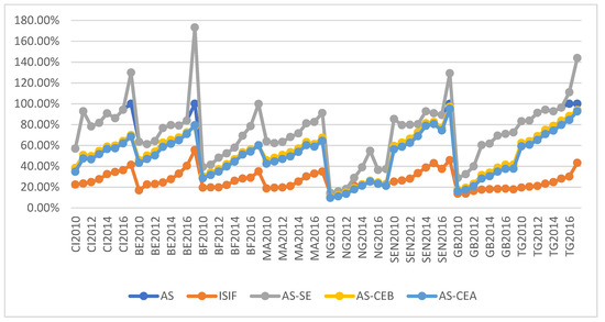
Figure 1.
ISIF, AS, AS–SE, AS–CEB, and AS–CEA for the sample.
We observe an apparent concordance between the scores for all the DMUs, as their patterns are highly similar.
Using these scores, we have further confirmed this visual information by performing three correlation analyses based on Pearson, Spearman, and Kendall’s Tau coefficients. It is worth noting that we have used these three analyses because previous Shapiro–Wilk tests for multivariate (see Table 8) and bivariate normality (see Table 9) significantly rejected the hypothesis of normality in all cases except for the pairwise (AS—AS–CEA) comparison. Table 10 presents the correlation matrix resulting from the correlation analyses.
Table 8.
Shapiro–Wilk Test for multivariate normality.
Table 9.
Shapiro–Wilk Test for bivariate normality.
Table 10.
Correlation matrix.
The analyses confirmed our visual findings. The five measures of financial inclusion, ISIF, and our four DEA-based ones, are concordant, as the three correlation coefficients are all strong and significant. We can therefore conclude that by using data envelopment analysis, we can obtain qualitatively suitable measures of financial inclusion.
5.2. Financial Inclusion Performance Level and Ranking in WAEMU
The second objective of this study was to use our proposed DEA-based composite score to assess the level of performance of the economies of WAEMU when it comes to financial inclusion. Looking at the union level, we have computed descriptive statistics of scores obtained from our five measures annually in Table 11. We have also performed two ANOVA analyses to determine whether there were differences in the annual averages. Note that d.o.f. stands for “degree of freedom”.
Table 11.
All financial inclusion measures by year.
We had already observed in the previous section that according to ISIF, the level of financial inclusion steadily increased during 2010–2017. However, the year-to-year rate of improvement was different. The four DEA-based scores lead to the same observation. The ANOVA tests were significant for most measures and further confirmed that fact. Moreover, most of the year-to-year improvement rates are of similar magnitude for all the measures.
We also looked at the performance at the country level. Table 12 presents descriptive statistics of scores obtained from our five measures for each country. We have also performed two ANOVA analyses to determine whether there were differences in the country averages from 2010 to 2017. Note that d.o.f. stands for “degree of freedom”.
Table 12.
All financial inclusion measures by economies.
We can observe that the ANOVA tests all significantly reject the hypothesis of equality of the average score for each country. Hence, on average, the performance of the countries has been different and heterogeneous. Let us recall that in an ANOVA test, the F-value is calculated as the ratio of variation between sample means over variation within the samples. The higher the F-value in an ANOVA is, the higher the variation between the sample means is relative to the variation within the samples. Therefore, when our ANOVA tests are significant, we can interpret high F-values as indicative of the discriminatory power of the corresponding measure. Indeed, high F-values here mean that the differences between the means for each economy are more significant.
From Table 12, based on the F-values, we can infer that the AS and AS–SE scores discriminate among countries less than ISIF, which discriminates less than AS–CEB and AS–CEA. This means that when using our measures to rank economies, we obtain stricter orders with AS–CEB and AS–CEA than with ISIF, and the orders from ISIF are stricter than the ones from AS and AS–SE.
We have then analyzed the evolution of each country’s performance from 2010 to 2017. Figure 2 (respectively Figure 3, Figure 4 and Figure 5) provides a visual illustration of the evolution of the financial inclusion level for each country according to the aggregate scores (AS) (respectively the super-efficiency scores (AS–SE), the benevolent cross-efficiency scores (AS–CEB), and the aggressive cross-efficiency scores (AS–CEA)).
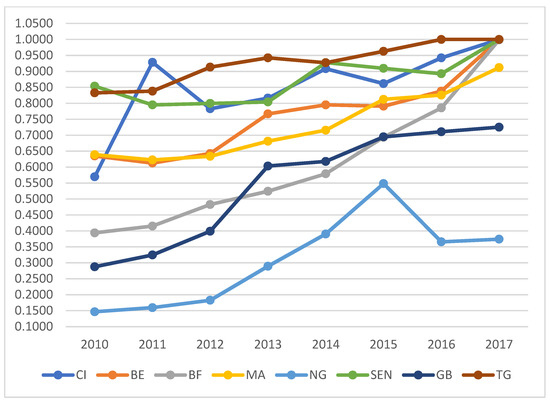
Figure 2.
AS from 2010 to 2017.
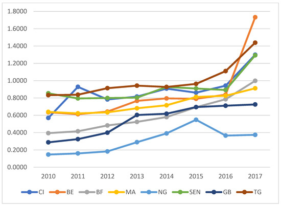
Figure 3.
AS–SE from 2010 to 2017.
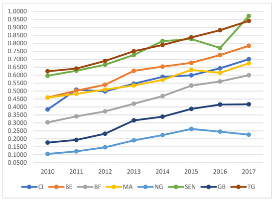
Figure 4.
AS–CEB from 2010 to 2017.
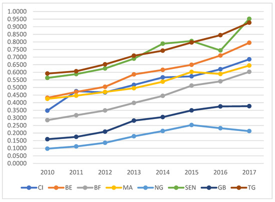
Figure 5.
AS–CEA from 2010 to 2017.
Let us recall that, according to the synthetic score ISIF, the situation at the level of each of the countries was heterogeneous. All of them had seen a continuous improvement in their performance between 2010 and 2015 but at different rates. This behavior is confirmed for two (AS–CEB, AS–CEA) of our four DEA-based measures. According to AS and AS–SE, the five top performers had a more unstable performance during those five years. Nevertheless, it is worth noting that this may also be because these scores are self-evaluation efficiency scores, which result in a lower discrimination power. Hence, we may affirm that the trends of the financial inclusion performance of the eight countries between 2010 and 2015 observed with ISIF are confirmed by the new DEA-based measures.
Again, according to ISIF, from 2015 to 2017, five of the countries (Benin, Burkina, Ivory Coast, Mali, and Togo) have continued their steady improvement; Senegal has taken a dip in 2016, which it has recovered since, while the Niger and Guinea-Bissau saw slight deteriorations in both 2016 and 2017. All our four-DEA based measures exhibit the same behavior for Benin, Burkina, Ivory Coast, and Togo (steady improvement); Senegal (dip in 2016, followed by recovery in 2017); and Niger (slight deteriorations in both 2016 and 2017). Regarding Mali, AS and AS–SE shows a steady improvement, while AS–CEA and AS–CEB hint at a dip in 2016, followed by a recovery the next year. Finally, Guinea-Bissau improved, followed by a stable performance in 2017. In summary, we observe a consensus among the five measures regarding the performance of six countries (Benin, Burkina, Ivory Coast, Senegal, Togo, and Niger) and a slight disagreement for the two remaining countries.
We finally used the five performance measures to rank the eight countries. Two rankings were performed. Table 13 summarizes the different rankings obtained according to the average score of five measures for the period of study. Table 14 summarizes the different rankings obtained according to the scores of the countries for the last year (2017) of the period of study for the five measures.
Table 13.
Rank—Country—Average measures.
Table 14.
Rank—Country—2017 measures.
On average (Table 13), the five measures do not rank the countries in the same positions. However, we can observe that the same four countries are consistently ranked in the first four positions by all five measures. These countries are Benin, Ivory Coast, Senegal, and Togo.
We can make the same observations when we only consider the year 2017. Although the actual positions are different, the same four countries identified previously occupy the first four positions for the rankings in Table 14. In addition, they are the only countries performing above the WAEMU average consistently for the study period. Furthermore, they are all equally placed first by AS, which means that their corresponding DMUs are all relatively efficient with respect to our sample of 64 DMUs.
5.3. Benchmarking Analysis
Using aggregate scores (ASs), which are also efficiency scores, we have subsequently performed a benchmarking analysis. This type of analysis aims to identify, in our sample, the decision-making units (DMUs) that are efficient and exhibit the best practices. The secondary goal is to identify, for each country that is not efficient, its reference set, which is a subset of the group of efficient DMUs that it must emulate in order to improve its efficiency.
DMUs whose efficiency scores are equal to 1 (100%) are the efficient ones. Hence, according to Table 4, the efficient DMUs in our sample were BE2017, CI2017, SEN2017, TG2016, and TG2017. In other words, four countries in the Union exhibit the best practices concerning financial inclusion: Benin, Senegal, Ivory Coast, and Togo. The first three reached that status only in the last year of the study, 2017, while Togo reached it in 2016 and maintained it the following year. It is worth noting that these four efficient countries were also identified in the previous subsection as being consistently ranked on average in the top four positions and performing consistently above average for our five measures.
Of our 64 DMUs, five were efficient. Hence, 59 were inefficient. We have observed how often our five efficient DMUs appear in the reference sets of these inefficient units. This results in SEN2017 being a reference country for 50 out of 59 non-efficient DMUs, followed, respectively, by TG2017 (32), TG2016 (15), BEN2017 (12), and CI2017 (6). In other words, concerning their relative efficiency, Senegal plays the role of leader in the economic union. Most non-efficient units must target it in part to improve their performance. Moreover, when we look at the DMUs from the last year of the study (2017), all the non-efficient units have Senegal in their reference set (Table 15). Indeed, the following four DMUs, namely BF2017, MA2017, NG2017, and GB2017, compared to the 64 units of our sample, would need to improve their performance. Our benchmarking analysis provides a reference set they can use to achieve that objective. Table 15 summarizes that information.
Table 15.
Benchmarking—Reference sets for non-efficient countries in 2017.
Table 15 provides, for each non-efficient DMU, its scores (column 2), the countries that form its reference set and the corresponding coefficient (column 3), and the current values of the financial inclusion indicator (columns 4 to 13). Using that information, the DMU can determine the virtual target country it has to aim at to achieve efficiency. More precisely, using the coefficient corresponding to the members of the reference set, policy-makers can calculate the exact value of each financial inclusion indicator of the target virtual country it has to emulate, which are the values that it must aim for (lines 3, 5, 7, 9, columns 4 to 13).
It is straightforward to see that the target values provide relevant and meaningful insight into how one can make changes or adjustments to improve performance. Now, it is true that some target values may come across as unrealistic, at least in the shorter term. For example, to attain efficiency, Guinea-Bissau would have to increase its rate of geographic penetration of electronic money services by more than 6000%; Niger would have to increase its rate of geographic penetration of microfinance services by more than 2000%. Nevertheless, beyond their actual figures, the target values still provide meaningful information regarding where to focus to improve performance.
5.4. Weight Analysis
We finally analyzed the optimal aggregation weights obtained from the CCR DEA models solved to calculate the AS composite scores. These optimal weights are presented in Table 16 below. Let us recall that aggregation weights represent the indicators’ relative importance. Using that interpretation, optimal weights from DEA models indicate the financial inclusion indicators that are the most important, or those who contribute the most to the level of performance of the DMUs.
Table 16.
DEA self-evaluation optimal weight by DMUs.
We can observe that several optimal weights are not significant for all the DMUs. There are also instances where only one significant weight is assigned. For example, we have optimal weights equal to 1 for all the DMUs related to Guinea-Bissau, CI2011, CI2012, or MA2010. A non-significant optimal weight would mean that the corresponding indicator is not essential to financial inclusion. In contrast, only one significant weight assigned would indicate that the corresponding indicator is the only one out of ten important or relevant to financial inclusion. Indeed, this does not hold in real life. These situations illustrate one of the limitations of the DEA methodology. Therefore, additional investigation is required where DEA with restrictions models (Greco et al. 2019; Angulo-Meza and Lins 2002) would be used.
Nevertheless, we can still interpret a non-significant optimal weight as indicative of potential areas of improvement. Countries must aim to increase the corresponding indicators while not deteriorating the indicators with significant weights to improve their overall performance.
Let us recall also that some of our indicators (geographic and demographic penetration) measure accessibility to financial services, or, in other words, the supply side of those services. In contrast, the others evaluate the utilization or the demand side.
In the earlier years of our period of study, financial inclusion was driven by the traditional financial services (banking and/or microfinance), either by their supply side, their demand, or a combination of both. Guinea-Bissau stayed in the same situation for the whole period: financial inclusion driven by the supply side of banking services. Ivory Coast also mainly relied on banking services until the country started to shift toward more electronic/mobile money services, especially the demand side. In this country, microfinance services do not appear to have ever been a driving force for financial inclusion. In Niger and Mali, financial inclusion was driven mainly by the supply side of banks in the early years, and banks and mobile money providers in recent years. In Benin, Burkina Faso, Senegal, and Togo, banking services, especially on the demand side, and microfinance services on both the supply and demand side have significantly driven financial inclusion.
All the countries in the Union have experienced a substantial shift toward mobile or electronic money service providers as drivers of financial inclusion in the later years of the period of study: Niger starting in 2013 on the supply side, Ivory Coast in the same year but more on the demand side, Mali in 2015 on the supply side, Benin in 2015 on the supply side, Senegal and Togo on both the demand and the supply sides, and finally Burkina Faso in 2017 on the supply side. These last remarks are consistent with the recent Global Findex survey, which found that in 2021, sub-Saharan Africa exhibits the highest rate of adults owning an account with a mobile money services provider.
6. Conclusions
In this study, we show through a case study on the economies of the West African Economic and Monetary Union (WAEMU) that the data envelopment analysis (DEA) methodology is an appropriate tool to build composite measures of the financial inclusion state of a country. Using that methodology, we have calculated efficiency, super-efficiency, and cross-efficiency measures that we have shown to correlate significantly with the PCA-based measures typically present in the literature. Moreover, the super-efficiency and cross-efficiency measures’ discrimination power among units is comparable to the PCA ones, making them suitable for ranking purposes.
We have confirmed that during the period of study, 2010–2017, the WAEMU experienced a steady increase in its level of inclusion. At the country level, the portrait of the situation is more mixed, with countries that have improved their levels during the whole period when others have experienced some bumps. We confirmed these observations on all measures statistically.
In addition, we performed a benchmarking analysis using the efficiency scores and their corresponding optimal weights and assessed the financial services that drive financial inclusion in each country. Specifically, we determined the countries that exhibit the best practices in financial inclusion in the sample. For the other countries, we identified the reference country they must emulate to improve their performance. In addition, we have described for each country which financial service sectors and which one of their demand and supply sides are driving forces for financial inclusion. Interestingly, we could observe that mobile or electronic money service providers were becoming a driving force of financial inclusion toward the end of our period of study. This latter fact is consistent with observations from the latest Global Findex survey in 2021.
Our study has some limitations which are essential to point out. First, from the methodology point of view, our work can be improved by using a DEA with weight restrictions models to ensure that more realistic optimal weights are obtained. In our analysis, we used ANOVA to assess whether there were differences in the averages by year and by economy. A better test to perform this work exists when one uses efficiency scores, as in the Simar–Zelenyuk test (Simar and Zelenyuk 2006). Future work should use this dedicated test to compare sample averages. Furthermore, we would need to incorporate in our model indicators of the third dimension of financial inclusion in WAEMU, which is quality. The DEA methodology should be validated further on additional samples, particularly from the Global Findex databases. More research will be needed to confirm the observations regarding the driving forces of financial inclusion in the WAEMU union.
Author Contributions
Conceptualization, P.M.T., M.D. and A.O.; methodology, P.M.T., M.D. and A.O.; software, M.D. and P.M.T.; validation, P.M.T., M.D. and A.O.; formal analysis, P.M.T., M.D. and A.O.; investigation, P.M.T., M.D. and A.O.; resources, P.M.T., M.D. and A.O.; data curation, P.M.T. and A.O.; writing—original draft preparation, P.M.T.; writing—review and editing, P.M.T., M.D. and A.O.; visualization, P.M.T., M.D. and A.O. All authors have read and agreed to the published version of the manuscript.
Funding
This research received no external funding.
Data Availability Statement
Publicly available datasets were analyzed in this study. These data can be found here: https://www.bceao.int/fr/content/la-base-des-donnees-economiques-et-financieres, accessed on 25 August 2019.
Conflicts of Interest
The authors declare no conflict of interest.
References
- Ahamed, M. Mostak, and Sushanta K. Mallick. 2019. Is Financial Inclusion Good for Bank Stability? International Evidence. Journal of Economic Behavior & Organization 157: 403–27. [Google Scholar]
- Alliance for Financial Inclusion. 2010. Mesurer l’inclusion Financière Pour Les Organismes Régulateurs: Conception et Réalisation d’enquêtes. Bangkok: Alliance for Financial Inclusion (AFI). [Google Scholar]
- Alvarez, Inmaculada C., Javier Barbero, and José L. Zofío. 2020. A Data Envelopment Analysis Toolbox for MATLAB. Journal of Statistical Software 95: 1–49. [Google Scholar] [CrossRef]
- Anarfo, Ebenezer Bugri, Joshua Yindenaba Abor, and Kofi Achampong Osei. 2020. Financial Regulation and Financial Inclusion in Sub-Saharan Africa: Does Financial Stability Play a Moderating Role? Research in International Business and Finance 51: 101070. [Google Scholar] [CrossRef]
- Angulo-Meza, Lidia, and Marcos Pereira Estellita Lins. 2002. Review of Methods for Increasing Discrimination in Data Envelopment Analysis. Annals of Operations Research 116: 225–42. [Google Scholar] [CrossRef]
- Aparicio, Juan, and Magdalena Kapelko. 2019. Enhancing the Measurement of Composite Indicators of Corporate Social Performance. Social Indicators Research 144: 807–26. [Google Scholar] [CrossRef]
- Arun, Thankom, and Rajalaxmi Kamath. 2015. Financial Inclusion: Policies and Practices. IIMB Management Review 27: 267–87. [Google Scholar] [CrossRef]
- Assaf, A. George, Carlos Barros, and Ricardo Sellers-Rubio. 2011. Efficiency Determinants in Retail Stores: A Bayesian Framework. Omega 39: 283–92. [Google Scholar] [CrossRef]
- Banker, Rajiv D., Abraham Charnes, and William Wager Cooper. 1984. Some Models for Estimating Technical and Scale Inefficiencies in Data Envelopment Analysis. Management Science 30: 1078–92. [Google Scholar] [CrossRef]
- Banker, Rajiv D., Robert F. Conrad, and Robert P. Strauss. 1986. A Comparative Application of Data Envelopment Analysis and Translog Methods: An Illustrative Study of Hospital Production. Management Science 32: 30–44. [Google Scholar] [CrossRef]
- Banque Centrale des États de l’Afrique de l’Ouest. 2018a. Evolution Des Indicateurs de Suivi de l’inclusion Financière Dans l’UEMOA Au Titre de l’année 2017. Dakar: Banque Centrale des États de l’Afrique de l’Ouest (BCEAO). [Google Scholar]
- Banque Centrale des États de l’Afrique de l’Ouest. 2018b. Rapport Annuel sur la Situation de l’Inclusion Financière Dans l’UEMOA Au Cours de l’année 2017. Dakar: Banque Centrale des États de l’Afrique de l’Ouest (BCEAO). [Google Scholar]
- Becker, William, Michaela Saisana, Paolo Paruolo, and Ine Vandecasteele. 2017. Weights and Importance in Composite Indicators: Closing the Gap. Ecological Indicators 80: 12–22. [Google Scholar] [CrossRef]
- Behzadian, Majid, S. Khanmohammadi Otaghsara, Morteza Yazdani, and Joshua Ignatius. 2012. A State-of the-Art Survey of TOPSIS Applications. Expert Systems with Applications 39: 13051–69. [Google Scholar] [CrossRef]
- Cámara, Noelia, and David Tuesta. 2014. Measuring Financial Inclusion: A Muldimensional Index. BBVA Research Paper, No. 14/26. Madrid: BBVA Research. [Google Scholar]
- Chakraborty, Subrata. 2022. TOPSIS and Modified TOPSIS: A Comparative Analysis. Decision Analytics Journal 2: 100021. [Google Scholar] [CrossRef]
- Charnes, Abraham, William W. Cooper, and Edwardo Rhodes. 1978. Measuring the Efficiency of Decision Making Units. European Journal of Operational Research 2: 429–44. [Google Scholar] [CrossRef]
- Chen, Yao, Wade D. Cook, and Sungmook Lim. 2019. Preface: DEA and Its Applications in Operations and Data Analytics. Annals of Operations Research 278: 1–4. [Google Scholar] [CrossRef]
- Cherchye, Laurens, and Timo Kuosmanen. 2004. Benchmarking Sustainable Development: A Synthetic Meta-Index Approach. WIDER Research Paper No. 2004/28. Helsinki: The United Nations University World Institute for Development Economics Research (UNU-WIDER). ISBN 9291906158. [Google Scholar]
- Cherchye, Laurens, Wim Moesen, and Tom Van Puyenbroeck. 2004. Legitimately Diverse, yet Comparable: On Synthesizing Social Inclusion Performance in the EU. JCMS: Journal of Common Market Studies 42: 919–55. [Google Scholar] [CrossRef]
- Cherchye, Laurens. 2001. Using Data Envelopment Analysis to Assess Macroeconomic Policy Performance. Applied Economics 33: 407–16. [Google Scholar] [CrossRef]
- Daraio, Cinzia, and Leopold Simar. 2007. The Measurement of Efficiency. In Advanced Robust and Nonparametric Methods in Efficiency Analysis: Methodology and Applications. Boston: Springer, vol. 4, pp. 13–42. [Google Scholar]
- Demirgüç-Kunt, Asli, and Leora Klapper. 2012. Measuring Financial Inclusion: The Global Findex Database. Policy Research Working Paper 6025: 1–61. [Google Scholar]
- Demirgüç-Kunt, Asli, Leora F. Klapper, Dorothe Singer, and Peter Van Oudheusden. 2015. The Global Findex Database 2014: Measuring Financial Inclusion around the World. World Bank Policy Research Working Paper, No. 7255. Washington, DC: World Bank Publications. [Google Scholar]
- Demirgüç-Kunt, Asli, Leora Klapper, Dorothe Singer, and Saniya Ansar. 2018. The Global Findex Database 2017: Measuring Financial Inclusion and the Fintech Revolution. Washington, DC: World Bank Publications. [Google Scholar]
- Demirgüç-Kunt, Asli, Leora Klapper, Dorothe Singer, and Saniya Ansar. 2022. The Global Findex Database 2021: Financial Inclusion, Digital Payments, and Resilience in the Age of COVID-19. Washington, DC: World Bank Publications. [Google Scholar]
- Dia, Mohamed, Amirmohsen Golmohammadi, and Pawoumodom M. Takouda. 2020a. Relative Efficiency of Canadian Banks: A Three-Stage Network Bootstrap DEA. Journal of Risk and Financial Management 13: 68. [Google Scholar] [CrossRef]
- Dia, Mohamed, Kobana Abukari, Pawoumodom M. Takouda, and Abdelouahid Assaidi. 2019. Relative Efficiency Measurement of Canadian Mining Companies. International Journal of Applied Management Science 11: 224–42. [Google Scholar] [CrossRef]
- Dia, Mohamed, Pawoumodom M. Takouda, and Amirmohsen Golmohammadi. 2020b. Assessing the Performance of Canadian Credit Unions Using a Three-Stage Network Bootstrap DEA. Annals of Operations Research 311: 641–673. [Google Scholar] [CrossRef]
- Dia, Mohamed, Pawoumodom M. Takouda, and Amirmohsen Golmohammadi. 2021. Efficiency Measurement of Canadian Oil and Gas Companies. International Journal of Operational Research 40: 460–88. [Google Scholar] [CrossRef]
- Doumpos, Michael, and Constantin Zopounidis. 2014. Multicriteria Analysis in Finance. Berlin/Heidelberg: Springer. [Google Scholar]
- Doyle, John, and Rodney Green. 1994. Efficiency and Cross-Efficiency in DEA: Derivations, Meanings and Uses. Journal of the Operational Research Society 45: 567–78. [Google Scholar] [CrossRef]
- Emrouznejad, Ali, and Guo-liang Yang. 2018. A Survey and Analysis of the First 40 Years of Scholarly Literature in DEA: 1978–2016. Socio-Economic Planning Sciences 61: 4–8. [Google Scholar] [CrossRef]
- Fosso Wamba, Samuel, Angappa Gunasekaran, Rameshwar Dubey, and Eric WT Ngai. 2018. Big Data Analytics in Operations and Supply Chain Management. Annals of Operations Research 270: 1–4. [Google Scholar] [CrossRef]
- Foster, James E., Mark McGillivray, and Suman Seth. 2013. Composite Indices: Rank Robustness, Statistical Association, and Redundancy. Econometric Reviews 32: 35–56. [Google Scholar] [CrossRef]
- Greco, Salvatore, Alessio Ishizaka, Menelaos Tasiou, and Gianpiero Torrisi. 2019. On the Methodological Framework of Composite Indices: A Review of the Issues of Weighting, Aggregation, and Robustness. Social Indicators Research 141: 61–94. [Google Scholar] [CrossRef]
- Greyling, Talita, and Fiona Tregenna. 2017. Construction and Analysis of a Composite Quality of Life Index for a Region of South Africa. Social Indicators Research 131: 887–930. [Google Scholar] [CrossRef]
- Guérineau, Samuel, and Luc Jacolin. 2014. L’inclusion Financière En Afrique Subsaharienne: Faits Stylisés et Déterminants. Revue d’économie Financière 116: 57–80. [Google Scholar] [CrossRef]
- Le, Thai-Ha, Anh Tu Chuc, and Farhad Taghizadeh-Hesary. 2019. Financial Inclusion and Its Impact on Financial Efficiency and Sustainability: Empirical Evidence from Asia. Borsa Istanbul Review 19: 310–22. [Google Scholar] [CrossRef]
- Lovell, C. A. Knox, Jesus T. Pastor, and Judi A. Turner. 1995. Measuring Macroeconomic Performance in the OECD: A Comparison of European and Non-European Countries. European Journal of Operational Research 87: 507–18. [Google Scholar] [CrossRef]
- Mahlberg, Bernhard, and Michael Obersteiner. 2001. Remeasuring the HDI by Data Envelopement Analysis. Available online: https://ssrn.com/abstract=1999372 (accessed on 4 August 2020).
- Melyn, Wim, and Willem Moesen. 1991. Towards a Synthetic Indicator of Macroeconomic Performance: Unequal Weighting When Limited Information Is Available. Public Economics Research Papers. Leuven: K.U.Leuven, Centrum voor Economische Studiën. [Google Scholar]
- Nardo, Michela, Michaela Saisana, Andrea Saltelli, and Stefano Tarantola. 2005. Tools for Composite Indicators Building. European Comission Ispra 15: 19–20. [Google Scholar]
- Nicoletti, Giuseppe, Stefano Scarpetta, and Olivier Boylaud. 2000. Summary Indicators of Product Market Regulation with an Extension to Employment Protection Legislation. Paris: OECD Publishing. [Google Scholar]
- Ouattara, Alassane, Pawoumodom M. Takouda, and Mohamed Dia. 2021. Un indice agrégé d’inclusion financière basé sur l’analyse par enveloppement de données (DEA) en contexte UEMOA. CESAG Working Papers. pp. 88–95. Available online: https://www.cesag.sn/images/CESAG_WORKING_PAPERS-A_Ouattara_et_al.pdf (accessed on 25 August 2019).
- Paradi, Joseph C., H. David Sherman, and Fai Keung Tam. 2018. Data Envelopment Analysis in the Financial Services Industry. Berlin/Heidelberg: Springer. [Google Scholar]
- Pearce, Douglas, and Claudia Ruiz Ortega. 2012. Financial Inclusion Strategies: Reference Framework. Washington, DC: World Bank Publications. [Google Scholar]
- Permanyer, Iñaki. 2011. Assessing the Robustness of Composite Indices Rankings. Review of Income and Wealth 57: 306–26. [Google Scholar] [CrossRef]
- Sarma, Mandira. 2008. Index of Financial Inclusion. Working Paper No 215. New Delhi: Indian Council for Research on International Economic Relations (ICRIER). [Google Scholar]
- Sarma, Mandira. 2012. Index of Financial Inclusion—A Measure of Financial Sector Inclusiveness. Working Paper. Delhi: Centre for International Trade and Development, School of International Studies, Jawaharlal Nehru University. [Google Scholar]
- Simar, Leopold, and Paul W. Wilson. 1998. Sensitivity Analysis of Efficiency Scores: How to Bootstrap in Nonparametric Frontier Models. Management Science 44: 49–61. [Google Scholar] [CrossRef]
- Simar, Leopold, and Paul W. Wilson. 2000. Statistical Inference in Nonparametric Frontier Models: The State of the Art. Journal of Productivity Analysis 13: 49–78. [Google Scholar] [CrossRef]
- Simar, Léopold, and Valentin Zelenyuk. 2006. On Testing Equality of Distributions of Technical Efficiency Scores. Econometric Reviews 25: 497–522. [Google Scholar] [CrossRef]
- Storrie, Donald, and Hans Bjurek. 2000. Benchmarking European Labour Market Performance with Efficiency Frontier Techniques. Discussion Paper FS I 00–211. Berlin: Wissenschaftszentrum Berlin für Sozialforschung. [Google Scholar]
- Takouda, Pawoumodom M., and Mohamed Dia. 2019. An Empirical Study of the Performance of Canadian-Owned Chains of Retail Stores. International Journal of Services and Operations Management 33: 512–28. [Google Scholar] [CrossRef]
- Takouda, Pawoumodom M., Mohamed Dia, and Alassane Ouattara. 2020. Levels of Financial Inclusion in the WAEMU Countries: A Case Study Using DEA. Paper presented at the 2020 International Conference on Decision Aid Sciences and Application (DASA), Sakheer, Bahrain, November 8–9; pp. 1274–78. [Google Scholar]
- Takouda, Pawoumodom Matthias, and Mohamed Dia. 2016. Relative Efficiency of Hardware Retail Stores Chains in Canada. International Journal of Operational Research 27: 275–90. [Google Scholar] [CrossRef]
- Takouda, Pawoumodom Matthias, Mohamed Dia, Alassane Ouattara, and Konan Vincent De Paul Kouadio. 2022. Evaluating How the Regulatory Ecosystem Promotes Entrepreneurial Activities in Africa. In Africa Case Studies in Operations Research: A Closer Look into Applications and Algorithms. Edited by Hatem Masri. Cham: Springer International Publishing, pp. 91–128. [Google Scholar] [CrossRef]
- Toma, Pierluigi, Pier Paolo Miglietta, Giovanni Zurlini, Donatella Valente, and Irene Petrosillo. 2017. A Non-Parametric Bootstrap-Data Envelopment Analysis Approach for Environmental Policy Planning and Management of Agricultural Efficiency in EU Countries. Ecological Indicators 83: 132–43. [Google Scholar] [CrossRef]
- Zins, Alexandra, and Laurent Weill. 2016. The Determinants of Financial Inclusion in Africa. Review of Development Finance 6: 46–57. [Google Scholar] [CrossRef]
Publisher’s Note: MDPI stays neutral with regard to jurisdictional claims in published maps and institutional affiliations. |
© 2022 by the authors. Licensee MDPI, Basel, Switzerland. This article is an open access article distributed under the terms and conditions of the Creative Commons Attribution (CC BY) license (https://creativecommons.org/licenses/by/4.0/).