Evidence of Stock Market Contagion during the COVID-19 Pandemic: A Wavelet-Copula-GARCH Approach

Abstract

In this study, we propose a wavelet-copula-GARCH procedure to investigate the occurrence of cross-market linkages during the COVID-19 pandemic. To explore cross-market linkages, we distinguish between regular interdependence and pure contagion, and associate changes in the correlation between stock market returns at higher frequencies with contagion, whereas changes at lower frequencies are associated with interdependence that relates to spillovers of shocks resulting from the normal interdependence between markets. An empirical analysis undertaken on six major stock markets reveals evidence of long-run interdependence between the markets under consideration before the start of the COVID-19 pandemic in December 2019. However, after the health crisis began, strong evidence of pure contagion among stock markets was detected.

1. Introduction

The escalation of the COVID-19 pandemic in 2020 posed a major challenge for financial markets. As the contagion spread from the city of Wuhan in China’s Hubei province to become a global pandemic, stock price volatility reached levels unseen since the Great Financial Crisis in 2007–2008. In finance, it is well known that such extreme values do not occur in isolation, and that financial shocks experienced in one market are often transferred to another.

In the literature, a large body of empirical works distinguished between two forms of contagion (see, for example, Wolf 1999; Forbes and Rigobon 2002; Pritsker 2001; Dornbusch et al. 2000). The first form is referred to as “interdependence” between economic systems, and emphasises spillovers resulting from the interactions between markets. Here, the transmission mechanism of shocks is triggered by interdependence across countries in relation to their real and financial linkages. The second form of contagion relates to the cross-market linkages generated by shocks on financial markets not linked to the observed changes in macroeconomic fundamentals, but primarily resulting from the investors’ behaviour. This form of contagion is at times referred to as “shift” or “pure” contagion. In the literature, theoretical models explaining this form of contagion are based on multiple equilibria, endogenous liquidity shocks affecting portfolio allocation, investor psychology, and capital market liquidity. For example, Masson (1998) presents a multiple-equilibria model wherein a crisis in one country can act as a sunspot for another. In this model, the shift from a good to a bad equilibrium is driven not by actual linkages between economic systems, but by investor expectations. Similarly, Hernández and Valdés (2001) propose a model wherein a crisis in one country causes a liquidity shock to market participants, and induces investors to rebalance their portfolios. Realigning the weightings of portfolio assets causes a sell-off of certain asset classes, which subsequently lowers asset prices in countries not affected by the initial crisis. In behavioural finance, theoretical models relate contagion to investors’ herding behaviour. In these models, investment decisions by market participants are influenced by the investment choices of others. For example, Bikhchandani and Sharma (2000) studied the social learning effects of actions taken by agents who act sequentially; the authors argue that when decisions are sequential, the earliest actions may disproportionately affect the choices of the following agents, thereby leading to herd behaviour.

In the literature, several empirical works have documented evidence of contagion due to financial or real economy shocks. Some of the most influential studies are those by Kaminsky and Reinhart (2000), Allen and Gale (2000), Bae et al. (2003), and Bekaert et al. (2005). The consensus in the literature agrees, however, that pandemic-related developments rarely cause stock market contagion. For example, Baker et al. (2020), looking back to 1900, discovered no evidence of cross-market linkages in relation to infectious disease outbreaks. Remarkably, the authors found that the Spanish flu—which infected an estimated 500 million people worldwide between 1918 and 1920, and claimed approximately 50 million victims—had only a limited impact on the financial markets. In striking contrast, the COVID-19 outbreak has massively impacted the real economy, driving many countries into recession. Unlike other pandemic-related developments, the COVID-19 outbreak has triggered a massive spike in uncertainty in financial markets. For example, in the U.S. stock markets, volatility levels in the first quarter of 2020 surpassed those last seen in October 1987 and December 2008 and, before that, in late 1929 and the early 1930s (see Baker et al. 2020).

Following such a significant worldwide impact, a growing body of literature is emerging on the economic effects of COVID-19 (see, for example, Akhtaruzzaman et al. 2021; Zhang et al. 2020). Shahzad et al. (2021) investigated the effects of COVID-19 on the aggregate stock performance of tourism firms in the U.S. markets. Abuzayed et al. (2021) investigated the systemic distress risk spillover between the global stock market and individual stock markets in the countries most affected by the COVID-19 pandemic. The authors observed that during the COVID-19 period, financial markets in Europe and North America transmitted and received a more marginal extreme risk to and from the entire global market than Asian stock markets. Similarly, Bouri et al. (2021) provided evidence of a dramatic change in the structure and time-varying patterns of the connectedness of returns across various assets (gold, crude oil, world equities, currencies, and bonds) around the COVID-19 outbreak (see also Conlon and McGee 2020; Yousaf et al. 2021; Yarovaya et al. 2020).

Partially motivated by these observations, the present study searches for fresh insights into the extent to which stock markets have been affected by the COVID-19 crisis, asking whether the apparent market transmission is actually the effect of contagion or interdependence. Following the seminal paper by Forbes and Rigobon (2002), we investigate whether correlations between different equity markets increased significantly during the peak of the COVID-19 outbreak. We argue that in order to be classified as contagion, the correlation between stock markets should increase during the crisis episode. In the absence of a surge in cross-market linkages, volatility spillover is better classified as market interdependence.

In this paper, we propose a novel methodology combining the benefits of wavelet series expansions with copula estimation. We label it the “wavelet-copula-GARCH” procedure, abbreviated as “WC-GARCH”. The procedure can be easily performed in two steps: The first stage involves using wavelet analysis to decompose the series of stock market returns into components associated with different scale resolutions. In the second step, the decomposed series of stock market returns act as input variables to estimate the transmission mechanisms of shocks using copula functions. Since modelling dependence by copula is sensitive to marginal model assumptions to allow for heteroskedasticity, autocorrelation, and volatility asymmetry, we follow Jondeau and Rockinger (2006) in estimating the marginal distributions using a GARCH-type model.

The main innovation of the suggested procedure is the combination of wavelet analysis with GARCH-type copula models. Wavelet analysis is a filtering method closely related to time series and frequency domain methods that transform the original data into different frequency components with a resolution matching its scale. Unlike time series and spectral analysis, which provide information only on the time domain and frequency domain, respectively, wavelet analysis decomposes the stock market return series with respect to both time and frequency domains simultaneously. This allows us to investigate whether financial markets respond differently in dissimilar time scales. For example, two stock markets may be highly correlated in the long run, but not in the short run. Analysing different frequency components of the series separately enables us to examine the stock markets over different time intervals (i.e., short-, medium-, and long-term), and allows an assessment of how the evolution of market connectedness has evolved over time, thus capturing the possible changes in the relationship. To analyse the strength of the co-movements between stock markets over different time intervals, we estimate a copula-GARCH-type model. Conditional copulas are extremely useful in financial applications because copula functions allow the separation of the marginal distributions from the dependence structure entirely represented by the copula function. This separation enables researchers to construct multivariate distribution functions, starting from given marginal distributions that avoid the common assumption of normality for either marginal distributions or their joint distribution function (Bartram et al. 2007). Moreover, copulas are invariant to strictly increasing transformations of the random variables, while asymptotic tail dependence is their important property.

The present study contributes to the literature in several ways: First, analysing daily returns for six large stock markets in the USA, Canada, the UK, Hong Kong, China, and Japan, evidence of significantly increasing interdependence among stock markets was unearthed since the start of the COVID-19 outbreak. Our results reveal evidence of contagion in line with Forbes and Rigobon’s (2002) definition: a significant increase in linkages among stock markets after a shock to one country as measured by the degree to which asset prices move together across markets relative to this co-movement in tranquil times. Second, evidence of contagion among stock markets constitutes an unprecedented event since, according to the literature (see Baker et al. 2020; Nippani and Washer 2004 among others), no previous infectious disease outbreak has impacted the stock market as forcefully as the COVID-19 pandemic. Most empirical studies agree that previous pandemics greatly affected stock market volatility, but only had a mild impact in terms of stock market contagion. The proposed methodological approach is the third contribution of the paper. The paper builds on previous works by Mensi et al. (2017), where wavelet methods and copulas were applied to commodity markets (see also Jiang et al. 2018, Ji et al. 2018), and Shahzad et al. (2016), who examined the interdependence of stock markets using wavelet and variational mode decomposition techniques. However, our procedure differentiates from the methods used in the related literature, since we combine wavelet decomposition with GARCH-copula models to be able to distinguish between different types of contagion between stock markets. The combination of wavelet decomposition and GARCH-copula models allows us to analyse the evolution of the correlation in the time–frequency space. Consequently, this paper freshly characterises the short-term and long-term dependencies between stock market returns.

The remainder of this study is organised as follows: Section 2 describes market contagion from a theoretical perspective. Section 3 presents the WC-GARCH model, whereas in Section 4 the estimation results are reported. Finally, Section 5 contains some concluding remarks.

2. Theoretical Considerations

Financial contagion as a result of a global event originating from a country and spreading to other countries or regions has long been an object of interest to economists. The consensus in the literature agrees on two main channels for the propagation of contagion: physical exposure, and asymmetric information. Contagion through physical exposure occurs when, after a negative shock in one market, investors rebalance their portfolios and sell assets in other markets. Therefore, a shock in one market causes instability in others, regardless of the underlying fundamentals (see Kyle and Xiong 2001). Contagion may also result from asymmetric information in financial markets; King and Wadhwani (1990) argue that traders in international financial markets face “signal extraction problems”. Traders from one country are only imperfectly informed about the situation in other countries; therefore, agents extract further information from observable stock price movements, reflecting other traders’ behaviour. However, imperfect information sparks confusion between price movements related to idiosyncratic shocks in a foreign country and price movements that also reveal changes in information about their home country. As a result, asymmetric information can trigger excessive price spillovers across borders, including stock market crashes.

In the literature, contagion has been empirically identified through the propagation of extreme negative returns and the related increase in market correlation with respect to normal times. A large body of research suggests that international financial market contagion has occurred in various economic and financial crises. For example, King and Wadhwani (1990) find evidence of an increase in stock returns’ correlation in the 1987 crash (see also Bekaert et al. 2005). Similarly, Calvo and Reinhart (1996) report evidence of contagion during the Mexican Crisis, and Baig and Goldfajn (1999) reach similar conclusions after investigating the stock market correlation during the East Asian Crisis. Hon et al. (2004) find evidence of contagion between the Nasdaq and the other stock markets after the dotcom bubble collapse in the United States. In the wake of the U.S. subprime market crisis in 2005, several papers have assessed the existence of contagion in financial markets. For example, Park and Shin (2020) investigated the foreign banks’ exposure during the crisis, and found that emerging market economies were more exposed to banks in the crisis-affected countries, suffering more capital outflows during the global financial crisis. Evidence of contagion was also found in developed economies by Dungey and Gajurel (2015) (see also Zhang et al. 2020). Mohti et al. (2019) investigated the impact of the U.S. subprime market crisis on the Eurozone debt crisis (see also Bashir et al. 2016).

Although recent research has greatly improved our understanding of contagion, scarce attention has been devoted to the impact of infectious disease outbreaks on stock markets. Most empirical works related to the impact of epidemics focus on disease-associated economic costs as a result of morbidity and mortality. For example, Siu and Wong (2004) provided evidence of the economic impact of the SARS epidemic in China, Hong Kong, and Taiwan. When we study financial markets, there is remarkably little literature on the subject. Notably, most of the available evidence reports the negligible impact of infectious diseases such as SARS, Ebola, swine flu, and Zika on stock markets.1 For example, Nippani and Washer (2004) examined the effect of the SARS outbreak on financial markets, and detected no evidence of contagion in stock markets in Canada, Hong Kong, Indonesia, the Philippines, Singapore, and Thailand. Similarly, Koo and Fu (2003) argue that despite the serious emotional distress caused by the SARS outbreak, the disease had limited impact in the affected regions (see also Siu and Wong 2004; Chen et al. 2007, 2018; Baker et al. 2012; Del Giudice and Paltrinieri 2017; Ichev and Marinč 2018). Macciocchi et al. (2016) investigated the effects of the Zika virus outbreak in several affected countries, and concluded that the impact of the virus on stock markets was only marginal.

Few studies have investigated the impact of the COVID-19 pandemic on financial market volatility. Attempts to understand the effects of COVID-19 on market volatility include a study by Baker et al. (2020), which identifies the current pandemic as having the greatest impact on stock market volatility in the whole history of pandemics. Similarly, Zaremba et al. (2020) examined the impact of government policy measures on stock market volatility (see also Goodell 2020); the authors suggest that stock market volatility increased more in countries where governments took strict policy actions—such as information campaigns and cancellation of public events—to curb the spread of disease. Furthermore, Zhang et al. (2020) found significant increases in volatility for U.S. stock markets in response to reports of COVID-19 cases and deaths in multiple countries.

3. The WC-GARCH Procedure

The proposed WC-GARCH procedure can easily be carried out in two steps: In the first step, a type of discrete wavelet transform (DWT) is applied to the stock market indexes in order break down the raw stock market returns into sub-returns series with different time-scales. Following this, in the second step, for each time bracket, sub-returns series of the obtained filtered series can be used to analyse correlations between stock markets using a copula-GARCH-GJR (1,1) model. The resulting procedure allows us to examine the correlation structure between stock markets at different timescales.

The two-step procedure to estimate the correlation in the time–frequency domain is described below in more detail.

Step 1: The Wavelet Series Expansion

The first step for implementing the WC-GARCH procedure involves applying the wavelet series expansion to the stock market return series. Wavelet analysis is a technique that decomposes a time series into small waves that begin at a specific point in time and end at a later specific point in time. In other words, the wavelet is a small wave or “wavelet” that can be manipulated to extract frequency components from a complex and non-stationary signal. Broadly speaking, the wavelet decomposition methodology involves recursively applying a succession of low-pass and high-pass filters to the stock market return series. This process allows the separation of its high-frequency components from the low-frequency ones (for more details see, for example, Benhmad 2013). The decomposition of the series can be obtained using a wavelet transform that is based on two filters, which are respectively called the “mother wavelet”:

$${{\displaystyle \int }}^{}\varphi \left(t\right)dt=1,$$

and the “father wavelet”:

$${{\displaystyle \int }}^{}\psi \left(t\right)dt=0.$$

From the theoretical point of view, the wavelet series expansion methodology is closely related to spectral analysis, where a time series is decomposed into a spectrum of cycles of varying lengths of a Fourier transform. Using spectral analysis, it is possible to identify the most important features of a time series, such as trends, business cycles, and seasonality (see Priestly 1981 for a review). Spectral analysis is therefore an important tool that can be used to extract the main oscillatory components of a series; however, a possible drawback of the methodology is the underlying assumption of stationarity of a series. This strong assumption is counterfactual in most applications to financial series. In this respect, wavelet analysis does not require any assumptions about the data-generation process for the return series under investigation, thus overcoming the limitations of techniques such as spectral and Fourier analysis (for more details see Ramsey 2002).

Since the use of wavelets is a well-established methodology, in this section we only introduce the concepts and definitions useful for our purposes. For a review of the theory and use of wavelets, see Percival and Walden (2000), Gençay et al. (2001), and Daubechies (1992).

If $f\left(t\right)\in L^2(ℝ)$ is a function (for $t=1,\dots ,T)$, the time dimensions can be expressed as a linear combination of a wavelet function:

$$f\left(t\right)={\displaystyle \sum }_k{s}_{j,k}{\varphi }_{j,k}\left(t\right)+{\displaystyle \sum }_k{d}_{j,k}{\psi }_{j,k}\left(t\right)+{\displaystyle \sum }_k{d}_{i-1,k}{\psi }_{j-1,k}\left(t\right)+\dots +{\displaystyle \sum }_k{d}_{1,k}{\psi }_{j-1,k}\left(t\right),$$

(1)

where the orthogonal basis functions ${\varphi }_{j,k }$ and ${\psi }_{j,k }$ are defined as:

$${\varphi }_{j,k}=2^{-j/2}\varphi \left(\frac{t-2^{j}k}{2^j}\right)$$

$${\psi }_{j,k}=2^{-j/2}\psi \left(\frac{t-2^{j}k}{2^j}\right).$$

In Equation (1), the representation j is the number of multiresolution components, $s_{j,k}$ are called the smooth coefficients, and $d_{j,k}$ are called the detailed coefficients. They are defined by:

$$s_{j,k}={{\displaystyle \int }}^{}f\left(t\right){\varphi }_{j,k}\left(t\right)dt,$$

(2)

$$d_{j,k}={{\displaystyle \int }}^{}f\left(t\right){\psi }_{j,k}\left(t\right)dt \mathrm{for} j=1,2,\dots J.$$

(3)

The magnitude of these coefficients reflects a measure of the contribution of the corresponding wavelet function to the total signal. The scale factor $2^j$ is also called the dilation factor, and controls the length of the wavelet (window), whereas the translation parameter $2^{j}k$ refers to the location, and indicates the nonzero portion of each wavelet basis vector. The basis wavelet function is stretched (or compressed) according to the scale parameter to extract frequency information (a wide window yields information on low-frequency movements, while a narrow window yields information on high-frequency movements), and moved on the timeline (from the beginning to the end) to extract time information from the signal in question.

The expression in Equation (2) presents the long-scale smooth components that are used to generate the scaling coefficients, whereas the differencing coefficients are generated by the wavelets in Equation (3). The resulting multiscale decomposition of Equation (1) can be simplified as:

$$F\left(t\right)=S_J+D_J+D_{J-1}+\dots +D_j+\dots +D_1,j=1,\dots ,J$$

(4)

where $D_j$ is the $j$th level wavelet and $S_J$ represents the aggregated sum of variations at each detail of the scale.

In Equations (1) and (4), the father wavelet reconstructs the smooth and low-frequency parts of a signal, whereas the mother wavelet function describes the detailed and high-frequency parts of a signal. In empirical applications to financial data, the father wavelet can be interpreted as the trend (smooth component) that is the longest timescale component of the series, and mother wavelets can be interpreted as the cyclical components around the trend. Therefore, the expression in Equation (4) provides a complete reconstruction of the signal partitioned into a set of j frequency components, so that each component corresponds to a particular range of frequencies. The low-frequency part can detect what in the literature has been referred to as “interdependence”, whereas the high-frequency part may reflect “pure” contagion. A similar interpretation was suggested in Gallegati (2012) (see also Huang et al. (2015)).

Step 2: WC-GARCH Model

The second step of the suggested procedure involves using the filtered series obtained from the j-level multiresolution decomposition to estimate the copula functions in the time–frequency framework. This second stage requires: (a) estimating the marginal distributions of the decomposed stock market series, (b) specifying the copula function, and (c) estimating the copula.

(a) Marginal Distributions

The copula estimation procedure used in this paper heavily relies on the results of Sklar’s theorem (see Sklar 1959). According to Sklar’s theorem, a two-dimensional joint distribution function G with continuous marginals F_X and F_Y has a unique copula representation, so that:

$$G\left(x, y\right)=C\left(F_x\left(x\right), F_y\left(y\right)\right),$$

and for a joint distribution function, the marginal distributions and the dependence structure described by a copula can be separated.

$\left\{D_{j,A}\right\}$ and $\left\{D_{j,B}\right\}$ represent the stochastic processes denoting the j decomposed signal obtained from the wavelet transform in Equation (4) for the stock market returns $\left\{R_A\right\}$ and $\left\{R_B\right\}$, respectively. Note that to simplify the notation, the t subscription is omitted wherever possible, at no detriment to the analysis. Their conditional cumulative distribution functions (CDFs) are $F_{D_{j,A}}\left(R_A;{\theta }_A\right)$ and $F_{D_{j,B}}\left(R_B;{\theta }_B\right)$, respectively. The conditional copula function is defined as $C\left(u_t,v_t\right)$, where the frequency component $u=F_{D_{j,A}}\left(R_A;{\theta }_A\right)$ and $v=F_{D_{j,B}}\left(R_B;{\theta }_B\right)$ are continuous variables in $\left(0,1\right)$.

Using Sklar’s theorem, for a given $D_j$ in Equation (4), the bivariate joint conditional CDF of $\left\{R_A\right\}$ and {$R_B$} can be written as:

$$G\left(R_A,R_B\right)=C\left(F_{D_{j,A}}\left(R_A,{\theta }_A\right),F_{D_{j,B}}(R_B,{\theta }_B);\pi \right)$$

(5)

where $\pi$ is a parameter vector for the copula, ${\theta }_A,{\theta }_B$ are parameter vectors for each marginal distribution, and $\theta -({\pi }^{\prime },{\theta }_A^{\prime },{\theta }_p^{\prime }$ is a parameter vector for the joint distribution. The expression in Equation (5) decomposes the joint distributions into marginal distributions, $F_{D_{j,A}}, F_{D_{j,B}}$, and a copula, C, representing the dependence structure among the frequency components for the stock market indices under consideration. Therefore, the expression in Equation (5) allows us to model marginal distributions and dependence structure separately. However, to make the expression in Equation (5) operational, the estimation of the marginal distributions is required. To obtain the marginal distributions of $D_j$ in Equation (4) the GARCH-GJR (1,1) model suggested by Glosten et al. (1993) can be used. Specifically, the model for the margins can be expressed as:

$$D_{j,t}=\mu +{\epsilon }_t,$$

(6)

$${\epsilon }_t=Z_t\sqrt{h_t}$$

(7)

$$h_t^2=\mathsf{\delta }+\alpha {\epsilon }_t^2+\gamma {\epsilon }_{t-1}^2{M}_{t-1}+\beta h_{t-1}^2$$

(8)

$$Z_t~GHD\left(\lambda ,\chi \right)$$

where Z_t is a generalized hyperbolic distribution with shape parameters $\lambda \mathrm{and} \chi .$ Equation (6) decomposes the returns into a constant, μ, and an innovation process, ε_t. The expression in Equation (7) defines this residual as a product of conditional volatility and innovation. Equation (8) describes the dynamics of conditional volatility, which is explained by the coefficients $\alpha , \beta ,$ and $\gamma$. The parameters measure the size effect and persistence of the shocks on volatility, respectively. The impact of the shocks on the conditional volatility is determined the sign of the parameter $\gamma$ of the dummy variable, M, such that $M_t=1$ if ${\epsilon }_t<0$ (bad news), and $M_t=1$ otherwise. Note that the WC-GARCH procedure is a general method that can be readily extended to any GARCH-type model. Therefore, we suggest experimenting with several types of GARCH specifications and selecting the model that best describes the data at hand.

(b) Copula Function

The marginal GARCH-GJR(1,1)-GHD parameter estimates in Equation (6) provide estimated values of the conditional cumulate distribution function for each frequency component $D_j.$ Therefore, the bivariate copula function with dependence parameter $\theta$ is expressed by the following function:

$$c\left(u_t, v_t\right)={\left(max\left\{u_t^{\theta }+v_t^{\theta }-1,0\right\}\right)}^{\frac{1}{\theta }},$$

(9)

where $\theta \ge 1$. Note that if $\theta \to 0$, then {R_A} and {$R_B$} are independent in $D_j$, whereas they are perfectly dependent in $\theta \to \infty$. The expression in Equation (9) is the Clayton copula; among different pair-copula families, the Clayton copula is preferred for financial data, since it allows for more asymmetric tail dependence in the negative tail than in the positive (for more details see, among others, Nikoloulopoulos et al. 2012).

(c) Estimation Method

Under the assumption that all condition CDFs are differentiable, from Sklar’s theorem the joint density function of $D_{j,A}$ and $D_{j,B}$ can be expressed as:

$$G\left(D_{j,A},D_{j,B}\right)=\frac{\partial G\left(D_{j,A},D_{j,B}\right)}{\partial D_{j,A}\partial D_{j,A}}=C\left(F_{D_{j,A}}\left(R_A,{\theta }_A\right),F_{D_{j,B}}(R_B,{\theta }_B)\right)\times f_{D_{j,A}}\left(R_A,{\theta }_A\right)\times f_{D_{j,B}}\left(R_B,{\theta }_B\right),$$

(10)

where $c\left(u_t, v_t\right)$ is the conditional copula density function in Equation (8). Thus, for each timescale $D_j$ in Equation (4), the bivariate conditional density function of $\left\{R_A\right\}$ and $\left\{R_B\right\}$ is represented by the product of the copula density and the two conditional marginal densities $f_{D_{j,A}}\left(R_A,{\theta }_A\right)$ and $f_{D_{j,B}}\left(R_B,{\theta }_B\right)$. From Equation (9) the log-likelihood function, $log\left(\theta \right)$, can be obtained as:

$$log\left(G\left(D_{j,A},D_{j,B}\right)\right)=log \left(c\left(u_t, v_t\right)\right)+log\left(f_{D_{j,A}}\left(R_A,{\theta }_A\right)\right)+log\left(f_{D_{j,B}}\left(R_B,{\theta }_B\right)\right)$$

(11)

To estimate Equation (10) we use the inference for the margin method suggested by Joe (1997), which involves first estimating the parameters of each univariate model via maximum likelihood, before the marginal CDFs are applied to the standardized residuals.

4. Data and Estimation Results

The data considered in this study are daily closing equity market price indices for six markets. Particularly, we consider the S&P 500 Composite Index (S&P 500) for the United States, the S&P TSX Composite Index, (S&P/TSX) for Canada, the FTSE 100 Price Index (FTSE 100) for the UK, the Nikkei 225 Stock Average Index (N225) for Japan, the Hang Seng Index (HIS) for Hong Kong, and the Shanghai Share Index (SSE) for China. These were selected as being representative of the largest stock markets in the world; they are therefore ideal for investigating the issue of contagion during the first COVID-19 wave.

The sample covers the period from 1 January 2014 to 8 August 2020. The period under consideration allows us to isolate shocks due to the COVID-19 pandemic since, by 2014, the impact of the Great Recession that started in 2005 with the subprime market crisis in the U.S. had completely vanished in most of the world.

Stock returns are calculated as the difference between the logarithms of the price index. Furthermore, the missing data arising from holidays and special events are bypassed by assuming them to equal the average of the previously recorded price and the subsequent one. Note that in this application, the U.S. stock market is used as a numeraire for the correlations. Therefore, below we consider the level of co-movements between the S&P 500 and the other stock markets listed above.

4.1. Multiscale Analysis of Correlation

In this section we present the results of estimating the WC-GARCH model. However, as a preliminary investigation, we take advantage of the time-scale decomposition property of the wavelet to calculate the multiscale correlation between the S&P 500 and other stock markets. Specifically, we use the wavelet coefficients in Equation (4) to obtain the wavelet variance, wavelet covariance, and wavelet correlation.

The wavelet variance decomposes the variance of a time series into components associated with different scales. Similar to their classical counterparts, we define ${\sigma }_{A }^2\left(D_j\right)$ as the wavelet variance, at scale j, of the process {$R_A$} with variance ${\sigma }_{A }^2$, and ${\sigma }_{B }^2\left(D_j\right)$ as the wavelet variance, at scale j, of the process {$R_B$} with variance ${\sigma }_{B }^2$. We also define the wavelet covariance between the processes {$R_A$} and {$R_B$}, at wavelet scale j, as the covariance between scale-j wavelet coefficients of {$R_A$} and {$R_B$} given by:

$${\sigma }_{A,B }({\lambda }_j)\simeq Cov\left\{D_{R_A,j}, D_{R_B,j}\right\}.$$

Therefore, the correlation coefficient is obtained as:

$${\rho }_{A,B}\left({\lambda }_J\right)\equiv \frac{{\sigma }_{A,B }({\lambda }_j)}{{\sigma }_{A }\left({\lambda }_j\right){\sigma }_B\left({\lambda }_j\right)}$$

The wavelet correlation coefficient ${\rho }_{A,B}\left({\lambda }_J\right)$ provides a standardized measure of the relationship between the two processes on a scale-by-scale basis and, as with the usual correlation coefficient between two random variables, we assume that |${\rho }_{A,B}\left({\lambda }_J\right)$| ≤ 1.

Since related empirical works have shown that a moderate-length filter of length eight is adequate to deal with the characteristic features of financial data (see Gençay et al. 2001), we use the Daubechies compactly supported least asymmetric (LA) wavelet filter (Daubechies 1992). Then, using the wavelet coefficients, we estimate the wavelet-unbiased pairwise correlation coefficients. For the choice of $\varphi$ and $\psi$ in Equation (1), the doublet wavelet function with length eight is used for this study.

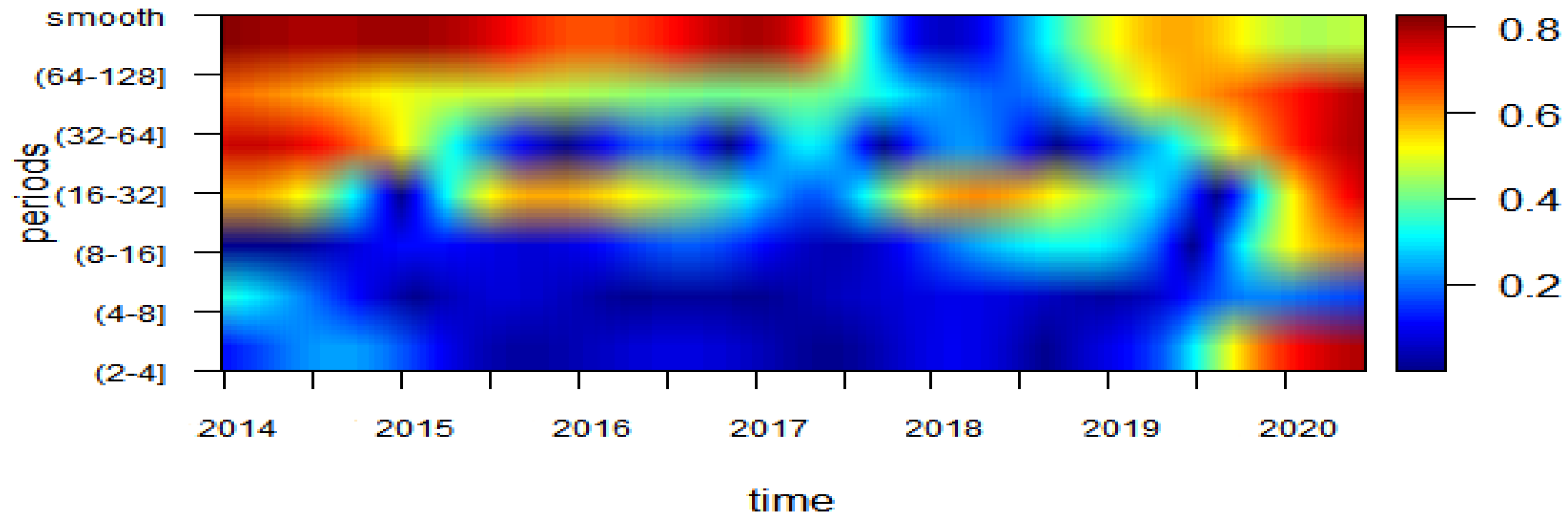
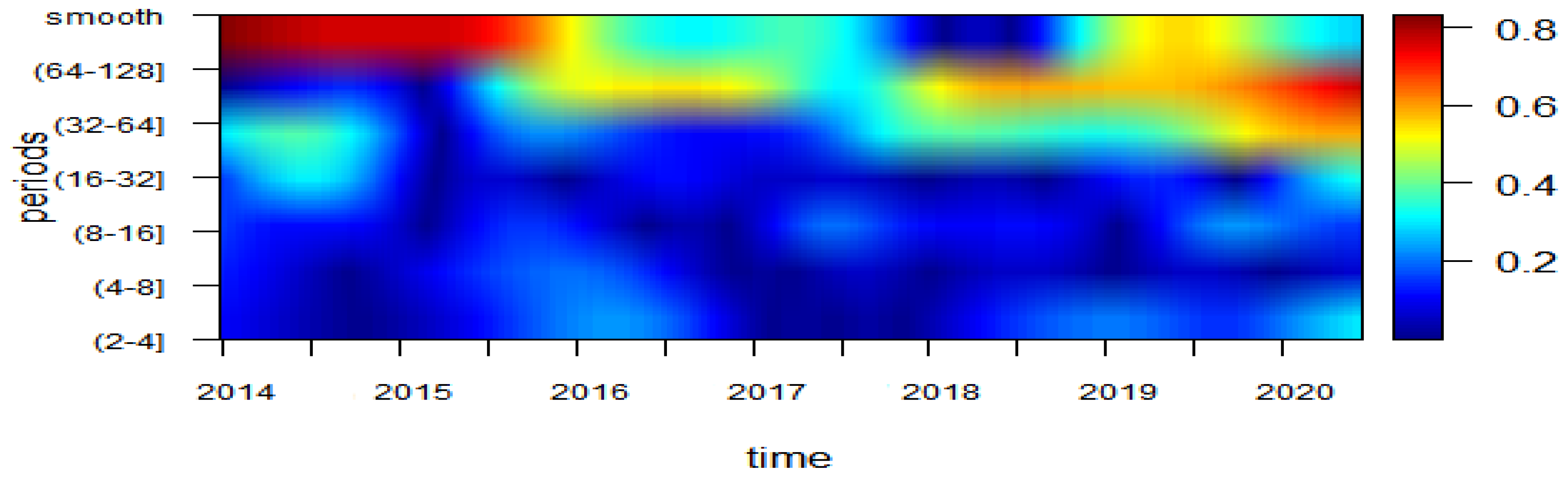
For the multiresolution level j, this study sets j = 6; thus, the highest frequency component D₁ represents short-term variations due to shocks occurring at a timescale of 2² = 4 days, and the next highest component D₂ accounts for variations at a timescale of 2³ = 8 days, near the working days of a week. Similarly, components D₃ and D₄ represent the midterm variations at timescales of 2⁴ = 16 and 2⁵ = 32 days, respectively. Finally, components D₅ and D₆ represent the long-term variations at timescales of 2⁶ = 64 and 2⁷ = 128 days, respectively. S₆ is the residual of the original signal after subtracting D₁, D₂, D₃, D₄, D₅, and D₆.

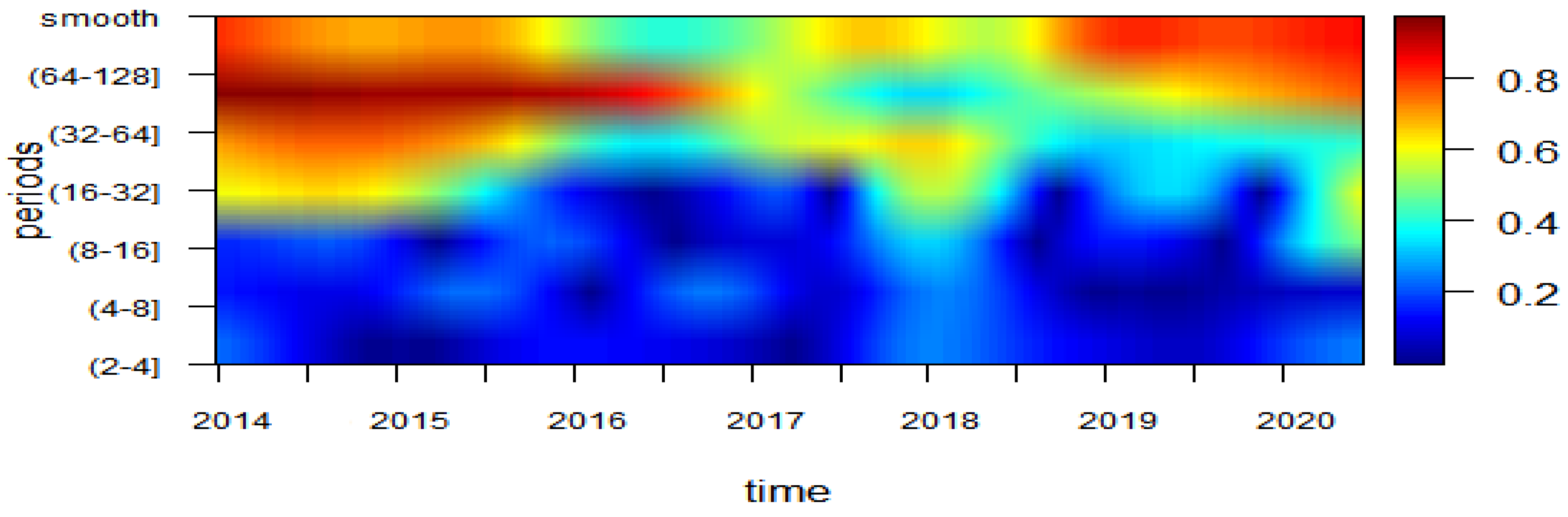
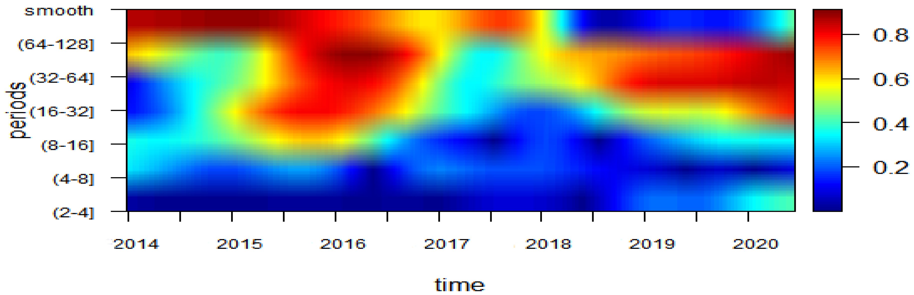
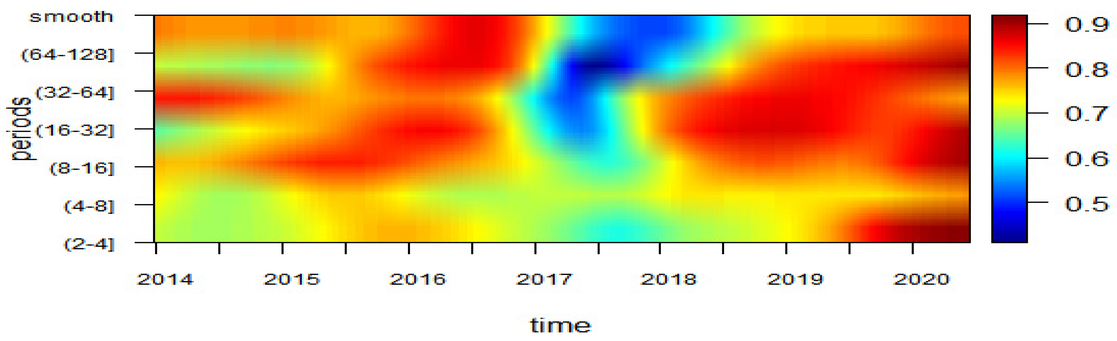
In Figure 1, Figure 2, Figure 3, Figure 4 and Figure 5, the correlation patterns between the S&P 500 and the other stock market indexes are presented in a time–frequency domain on a scale-by-scale basis. For ease of interpretation, the left-hand horizontal axis is transformed to show the number of days in which the scale moves from low to high wavelengths. The heat maps indicate the increasing strength of the correlation among the stock market indices as they move from blue (lowest correlation) to red (highest correlation).

Before interpreting the results of the correlation analysis, one issue that still has to be resolved is the following: for how many days should the increase in correlation between two stock markets last to be classified as “pure” contagion? This, in turn, gives us a definition of “interdependence”. Theoretical literature offers only limited help on this matter. According to the market efficiency hypothesis (EMH), the stock market prices should reflect all of the information made available to market participants at any given time (see Fama 1970). The EMH, therefore, implies that the transmission of shocks due to contagion in international financial markets should not exist in the long run. Based on these considerations, several papers suggest that the transmission of shocks due to contagion in international financial markets should be very fast, and should die out quickly. For example, Gallegati (2012) suggests that to be classified as “pure” contagion, the increase of correlation should generally not exceed one week (see also Dewandaru et al. 2016). However, in this paper, we argue that the COVID-19 pandemic spiked the uncertainty unseen in previous crises. As argued by Baker et al. (2020), the period considered in this study was a time of great uncertainty relating to almost every aspect of everyday life: the infectiousness and lethality of the virus, the availability and deployment of antigen and antibody tests, and the capacity of healthcare systems to meet an extraordinary challenge. In the light of these arguments, we suggest that the definition of “pure” contagion adopted in the related empirical studies should be taken more liberally. Hence, we assume that the first five wavelet scales provide a realistic measure of contagion, as these scales are associated with changes of up to 64 days in correlation shifts. Accordingly, in this paper, “pure” contagion is measured by wavelet coefficients D₁, …, D₅, whereas “interdependence” is measured by the D₆ scale and the trend, S₆.

From Figure 1, Figure 2, Figure 3, Figure 4 and Figure 5, there is clear evidence of long-run interdependence between the U.S. stock market and the other markets before the start of the COVID-19 pandemic in December 2019. Specifically, starting with the correlation between the U.S. and the U.K. markets, Figure 1 shows no sign of co-movements for the first 8–16 days (i.e., dark blue colour indicates a correlation no greater than 0.2), but the correlation increases in the time scale D₆ between January 2014 and June 2017 (i.e., the red colour corresponds to a correlation coefficient of 0.8). Similarly, in Figure 2, it appears that the U.S. and Japanese stock markets have stronger long-term co-movements since, once again, we see the red colour in the 64–128 timescale. As for the correlation between the U.S. and China, weak correlation (dark blue and light blue colour) can be seen for the shortest timescale (i.e., D₁–D₃), as highlighted in Figure 3.

Signs of fundamental-based contagion between the U.S. and Chinese stock markets can also be observed in Figure 4, where the estimated correlation coefficient is very high only for the timescale D₆ before 2016, and lower afterwards. The estimated correlation coefficient during the COVID-19 outbreak is interestingly consistent with our definition of “contagion” only for the timescale D₅, but is a borderline case of “interdependence” since in Figure 4 the red colour appears only for the longest timescales. Finally, the correlation between the stock markets in the U.S. and Canada, shown in Figure 5, indicates persistent co-movements between these financial markets, since Canada has close commercial and financial ties to the U.S. economy.

Overall, the results in Figure 1, Figure 2, Figure 3, Figure 4 and Figure 5 suggest that before the COVID-19 pandemic started, the transmission mechanism of shocks was related to normal dependence between markets, due to trade links and geographical position. Therefore, the type of transmission mechanism of shocks that characterised the period before the health crisis began seems better described as “interdependence” (see Forbes and Rigobon 2002).

Once the impact of the COVID-19 pandemic was felt worldwide, financial assets were immediately repriced. Panic spread throughout all of the major financial markets, as indicated by the wavelet power of pairwise analysis analysed in the lower scale brackets. Put differently, the co-movements (either positive or negative) seem to have been stronger during the COVID-19 pandemic in most of the series under consideration. Specifically, with the notable exception of Japan, the financial markets under consideration showed significant dominant signs of co-movement at periods of high frequency up to 64 days in length. In the case of the UK–Canada correlation, the market contagion appears even stronger, as indicated by the red colour in Figure 1 and Figure 5.

The results of the wavelet analysis in Figure 1, Figure 2, Figure 3, Figure 4 and Figure 5 reveal a degree of co-movement between the U.S. and other financial markets, suggesting that a parametric analysis may reveal more insights into the contagion effects during the COVID-19 outbreak.

4.2. WC-GARCH Procedure Estimation Results

Once the filtered series were extracted in the second step of our analysis, appropriate univariate GARCH models were estimated for the six stochastic processes under consideration. Comparing a number of GARCH-type models, we concluded that a GJR-GARCH model with a GHD distribution for the innovation terms was the specification that best fit the data under consideration. To investigate the effects of the COVID-19 pandemic, the sample under consideration was split into two subperiods: the first with $T=1465$ including data from 2 January 2014 to 29 November 2019; and the second subperiod with a sample of $T=172$ including observations from 2 December 2019 to 8 August 2020.

The WC-GARCH procedure suggested in Section 3 involves estimating a total of $\left(6\times D_j\right)=36$ GARCH-GJR (1,1) models for each subperiod, generating a staggering total of 72 models to be estimated. To save space, the estimation results are not reported here, but they are available upon request. However, to give an idea of the magnitude of the estimated coefficients for the conditional variance equations, the estimation results for the marginal distributions for the six stock markets under consideration in the two subperiods are reported in

Table 1. Estimation results of the single-equation models for the stock market indices under consideration before the COVID-19 outbreak.

	GSPTSE	GSPC	FTSE 100	HIS	SSE	N225
$\alpha$	0.145 **	0.343 **	0.324 *	0.107 *	0.077 *	0.201 *
	(0.044)	(0.167)	(0.002)	(0.049)	(0.003)	(0.011)
$\beta$	0.839 *	0.652 *	0.674 **	0.881 *	0.907 *	0.791 **
	(0.016)	(0.109)	(0.241)	(0.203)	(0.310)	(0.360)
$\gamma$	−0.708 *	−0.325 **	−0.258 **	−0.526 *	0.301 **	−0.685 *
	(0.154)	(0.112)	(0.159)	(0.017)	(0.171)	(0.291)
ARCH Lag (10)	2.624	5.161	4.599	3.233	3.923	3.452
	[0.417]	[0.195]	[0.257]	[0.396]	[0.403]	[0.368]

Note: The table reports the estimation results of the GARCH-GJR (1,1) for the stock markets under consideration. Squared brackets indicate the p-values; standard errors are reported below the estimated coefficients. Note that * and ** indicate significance at 1% and 5%, respectively. The tests for autocorrelation for the estimated models are also reported.

and

Table 2. Estimation results of the single-equation models for the stock market indices under consideration after the COVID-19 outbreak started.

	GSPTSE	GSPC	FTSE 100	HIS	SSE	N225
$\alpha$	0.084 **	0.034 **	0.203 *	0.062 *	0.076 *	0.191 *
	(0.033)	(0.156)	(0.013)	(0.360)	(0.008)	(0.020)
$\beta$	0.902 *	0.905 *	0.705 *	0.917 *	0.920 *	0.814 **
	(0.005)	(0.098)	(0.011)	(0.214)	(0.321)	(0.371)
$\gamma$	0.636 *	−0.397 *	−0.330 **	−0.598 *	0.228 **	−0.757 **
	(0.143)	(0.101)	(0.148)	(0.028)	(0.182)	(0.301)
ARCH Lag (10)	2.364	4.649	4.144	2.913	3.534	3.110
	[0.432]	[0.235]	[0.327]	[0.476]	[0.354]	[0.308]

Note: The table reports the estimation results of the GARCH-GJR (1,1) for the stock markets under consideration. Squared brackets indicate the p-values; standard errors are reported below the estimated coefficients. Note that * and ** indicate significance at 1% and 5%, respectively. The tests for autocorrelation for the estimated models are also reported.

.

Table 1 and Table 2 present the GARCH-GJR (1,1) parameter estimates for models estimated for the period before and during the COVID-19 outbreak, respectively. From Table 2, it appears that stock market indices are highly persistent, since the magnitude of the estimated parameters $\beta$ is relatively high for all of the estimated series. In Table 1 and Table 2, bad news also appears to impact stock market volatility, since all of the estimated $\gamma$ values significantly differ from zero. Furthermore, the diagnostic tests included at the bottom of Table 1 and Table 2 reject the null hypothesis of autocorrelation up to the 10th lag order.

Finally, in Table 2, all of the estimated $\beta$ coefficients appear greater in magnitude than those in Table 1, indicating that the COVID-19 outbreak increased persistence in the stock markets. On the other hand, the estimated coefficients for $\alpha$ and $\gamma$ in Table 2, on average, do not vary much with respect to those in Table 1.

Table 3. WC-GARCH-GJR (1,1) estimation results before the COVID-19 outbreak.

	D1 (2–4 Days)	D2 (4–8 Days)	D3 (8–16 Days)	D4 (16–32 Days)	D5 (32–64 Days)	D6 (64–128 Days)
FTSE 100	0.433	0.476	0.513	0.570	0.818	0.769
N225	0.056	0.114	0.178	0.359	0.456	0.782
SSE	0.062	0.067	0.041	−0.187	0.269	0.414
HIS	0.144	0.186	−0.331	−0.407	0.431	0.584
S&P TSX	0.596	0.674	0.563	0.631	0.762	0.863

Note: The table reports the WC-GARCH results that give the estimated correlations between the S&P 500 and the other stock market indices by frequency. The timescales are 2–4, 4–8, 8–16, 6–32, 32–64, and 64–128 days—defined as D₁, D₂, D₃, D₄, D₅, and D₆, respectively—between the U.S. and the other stock markets under consideration.

and

Table 4. WC-GARCH-GJR (1,1) estimation results during the COVID-19 pandemic.

	D1 (2–4 Days)	D2 (4–8 Days)	D3 (8–16 Days)	D4 (16–32 Days)	D5 (32–64 Days)	D6 (64–128 Days)
FTSE 100	0.582	0.617	0.652	0.768	0.832	0.856
N225	0.172	0.148	0.209	0.226	0.212	0.219
SSE	0.271	0.228	0.370	0.352	0.417	0.433
HIS	0.191	0.216	0.257	0.242	0.245	0.237
S&P TSX	0.645	0.724	0.746	0.758	0.824	0.876

Note: The table reports the WC-GARCH results that give the estimated correlations between the S&P 500 and the other stock market indices by frequency. The timescales are 2–4, 4–8, 8–16, 6–32, 32–64, and 64–128 days—defined as D₁, D₂, D₃, D₄, D₅, and D₆, respectively—between the U.S. and the other stock markets under consideration.

present the results of the pairwise correlation in the time–frequency domain between the S&P 500 and the other stock market returns obtained using the suggested WC-GARCH procedure.

In Table 3, the pairwise dynamic correlations for the pre-COVID-19 period are reported. The results in Table 3 conform to the definition of “interdependence” (or fundamental-based contagion) since, in general, looking at columns two, three, and four, it is clear that during the pre-COVID 19-crisis period the tail dependence was relatively weak in the short-run timescales, but increased with the timescale length (i.e., timescale D₅ and D₆). Particularly, tail correlations are rather low up to 16 days, (timescales D₁, D₂, and D₃), but increase in the 32–128-day timescales (timescales D₅ and D₆). Strangely, for timescale D₄, in column five, the correlations appear higher for all of the markets.

Looking now, the tail dependence between different stock markets, contagion (timescales D1–D3) during the pre-COVID 19 period between the S&P 500 and the other stock markets was relatively low for the N225, SSE, and HIS, and higher for the FTSE 100 and SPTSX. These results again conform to the definition of fundamental-based interdependence, where a shock to the U.S. spreads to a neighbouring market—such as Canada—because of the normal interdependence between these economies. The UK economy is also closely related to the U.S. economy; therefore, shock transmissions are expected to be higher than for those for Asian markets.

The interdependence-type of correlation during the pre-COVID-19 period is even clearer when we examine the tail dependence in the longest timescales (D₅ and D₆). The UK and Canada correlate highly with the U.S. for the longest timescale brackets. Looking now at the remaining stock markets, in this case the correlation also increases with the timescale. For example, the correlation between the U.S. and Japan’s stock markets was approximately 0.5 in D₅, and increased to approximately 0.8 in D₆, whereas Hong Kong’s correlation was approximately between 0.4 and 0.6. China’s correlation varied substantially, and was eventually slightly lower than Japan’s, at approximately 0.4 in D₆.

The picture dramatically changes during the COVID-19 period, since in Table 4 tail dependency increases in the timescales D₁ and D₂ (i.e., 2–8 days) for all of the stock markets under consideration, thus suggesting the existence of “pure” contagion even according to the strict criteria adopted by Gallegati (2012) and Dewandaru et al. (2016). Looking at longer time brackets (i.e., timescales D₃ and D₄), volatility spillovers are still evident between the S&P 500 and the other stock markets after a shock for up to 32 days; this is true for all of the markets except for the HIS. Looking at the long run (i.e., timescales D5 and D6), the picture completely changes, as for most pairwise stock market indices the estimated correlation coefficients are smaller or approximately the same. Taken together, these results confirm our hypothesis that the COVID-19 pandemic was a major source of contagion between markets. The high increase in the market correlations was obviously not linked to observed changes in macroeconomic fundamentals, but was mainly the result of the behaviour of investors or other financial agents.

5. Discussion and Comparison with Previous Results

What do we learn from the WC-GARCH procedure? Stock market contagion has important consequences for financial stability as well as portfolio management, since it affects optimal asset allocation, risk measurement, and asset pricing. However, standard time domain techniques can face problems in identifying contagion from other forms of shock transmission, because of the inability of these methodologies to combine information from both time and frequency domains. The modelling issues related to the analysis of co-movements between financial markets are well documented by the variety of econometric procedures used in empirical studies to investigate financial contagion. They include testing for changes in correlation coefficients (King and Wadhwani 1990; Lee and Kim 1993), ARCH and GARCH models (Billio and Caporin 2010), co-integration- estimating models (e.g., Chiang et al. 2007; Gallo and Otranto 2008; Voronkova 2004; Yang et al. 2003), limited dependent variable models (Eichengreen et al. 1996; Kaminsky and Reinhart 2000), nonlinear models (Gallo and Otranto 2008), and factor models (Corsetti et al. 2005). This paper argues that most of these models can describe only the average behaviour of the correlation patterns, since standard time-series models do not allow for more than two timescales: the short run, and the long run. According to theoretical models, shock transmission due to contagion should be rapid, and should die out quickly due to arbitrage opportunities in different markets, but “how fast is fast?” is a fundamental question in practical applications. In this respect, by applying a wavelet decomposition of the stochastic processes, the suggested procedure provides a complete reconstruction of the signal partitioned into a set of j frequency components. Each component corresponds to a particular range of frequencies. For example, the low-frequency part can be associated with what the literature has defined “interdependence”, and the high-frequency part can reflect “pure” contagion. Available literature confirms the effectiveness of adopting wavelet analysis in accounting for the difference between short- and long-term investors (see, for example, Yazgan and Özkan 2015; Yogo 2008; Gallegati 2012; Ranta 2013; Conlon et al. 2018).

Our main results have several implications: First, by analysing the tail correlation between markets in the pre- and post-COVID-19 subperiods, we can argue that contagion between the U.S. stock markets and the other five largest markets in the world peaked during the pandemic. Similar results were also reported by Okorie and Lin (2021), where fractal contagion effects were detected among major stock markets. Accordingly, portfolio managers and investors can utilise the results of this study to inform their decisions to monitor and manage portfolio risk effectively. Second, the results in Table 3 and Table 4 suggest that portfolio risk evaluation should consider extreme tail dependence between the stock markets during times of global distress, such as the COVID-19 pandemic. Ignoring market risk due to contagion may underestimate the level of systematic risk and, thus, mislead risk management strategies. In this respect, as the largest stock market in the world, the U.S. can be considered to be a major player in transmitting marginal tail risk to other markets during the COVID-19 subperiod, affecting the benefits of stock portfolio diversification during stress periods. Third, although COVID-19 first spread in China, we found that the contagion between the U.S. and the Chinese stock market was relatively low. This was also the case for other major Asian stock markets. Accordingly, portfolio managers seeking to minimise risk should consider these results when building portfolios. Finally, our results may also inform regulators and policymakers, who should consider the increase in dependence during times of market distress as a potential risk to financial stability. Accordingly, supervisory policies should aim to prevent extreme risk shocks from spreading to global stock markets in order to maintain domestic financial stability, especially if future COVID-19 waves emerge.

6. Conclusions

In this study, we proposed a novel procedure to investigate the occurrence of cross-market linkages during the COVID-19 pandemic. The predominant novelty of our model lies in combining wavelet analysis with copula estimation. In other words, the decomposed series obtained from the wavelet spectrum analysis is adopted in order to estimate a copula-GARCH model. An interesting feature of the WC-GARCH procedure is its ability to unveil relationships between stock market returns in the time–frequency domain, facilitating a simultaneous assessment of the relationship between markets at different frequencies and the evolution of these links over time. In this respect, the procedure provides an alternative representation of the correlation structure of stock market returns on a scale-by-scale basis.

To investigate the market linkages, we distinguish between regular “interdependence” and “pure” contagion, and associate changes in correlation between stock market returns at higher frequencies with contagion—which is a form of dependence that does not exist in tranquil periods, but occurs only during periods of turmoil. On the other hand, changes at lower frequencies are associated with interdependence that relates to the impact of shocks resulting from the normal dependence between markets, and refers to the dependence that exists in all states of the world due to trade links and geographical position. The estimation results reveal evidence of long-run “interdependence” between the markets under consideration before the start of the COVID-19 pandemic in December 2019. However, strong evidence of “pure” contagion between stock markets was detected as the health crisis began.

A possible limitation of our study is that we consider only the univariate GARCH model for our procedure. Future work should look at the multivariate GARCH in order to extend the analysis to volatility spillover among stock markets. Nevertheless, our results carry important implications, since they reveal that despite the policy measures instituted after the financial crisis of 2007–2008, measures are still required to mitigate the impact of shocks on financial markets. The COVID-19 pandemic is the first health crisis that has the potential to trigger devastating effects similar to those witnessed during the global financial crisis, which was arguably the first truly major global financial crisis since the Great Depression of 1929–1932. The subprime financial crisis originated in the United States in a relatively small segment of the lending market, but it rapidly spread across virtually all countries in the world. In this respect, if lessons have to be learned from past experience, evidence of long- and short-run cross-market linkages constitutes a wake-up call highlighting the need for policy measures to mitigate contagion.