Price Discovery and Learning during the German 5G Auction

Abstract

The auctioning of frequency has to comply with a multitude of requirements in order to guarantee a transparent and efficient process. The German Federal Network Agency (Bundesnetzagentur) has opted for a design that provides participants with information on the highest bid after each round for every band along with information on the bidder. We evaluate the price formation efficiency in this setup to see how fast prices become informative about the final auction value. We find that prices are partially informative right from the beginning which allows us to conclude that participants were able to learn fast from their competitors’ bidding behavior and validates the choice of the agency to implement the auction in the present format.

1. Introduction

With the introduction of the latest telecommunication standard for broadband cellular networks, 5G, the speed at which data transmission is possible has reached a new peak. Telecommunication companies all over the world are racing to be among the first to provide their clients with the latest technology. First, however, these companies have to acquire a spectrum of frequencies which they are allowed to use for their offered services. While some countries assign these frequencies to their telecommunication firms or hold administrative hearings (often referred to as “beauty contests”) such as China or Japan (Krempl 2019), most governments rely on auctions to achieve an efficient distribution of the spectrum among national providers. These frequency auctions are capable of generating a substantial revenue: In the United Kingdom, the UMTS (Universal Mobile Telecommunications System) auction’s revenue equaled 2.5% of the country’s gross domestic product in 2000 (Felder 2004). Similarly, the German UMTS auction raised 99.37 billion Deutsche Mark (roughly 50 billion Euro).

Germany has a long history of auctioning spectrum rights, having been the first country to do so in Europe in 1996 (Nett 2019). To accommodate the requirements of the new 5G technology, another auction was conducted in 2019 to allocate new frequencies in the n78 band1 used for the new standard. The German spectrum auction design has been used and improved upon multiple times. Several authors refer to it as tested and functional and come to the conclusion that it provides an efficient allocation of the available spectrum (for example Cramton and Ockenfels 2017; Nett 2019). Ultimately, the participating telecommunications companies paid a total of 6.55 billion Euro for their licenses. In this article we set out to analyze the price formation process and the learning of the market participants during the 5G auction. This allows us to evaluate the efficiency of the auction from a market microstructure point of view.

The analysis of price formation processes is at the core of market microstructure analysis. An influential early study is Walras (1954) who describes a tâtonnement process, the tentative, step-by-step procedure where market participants learn about the fundamental value which is revealed at the end. In the context of financial markets, stock market auctions are in the focus following the work of Biais et al. (1999) who analyze the pre-opening auction at the Paris Bourse. They document that orders become increasingly informative as the auction goes on and that the learning rate increases as the pre-opening auction gets closer to its end. Biais et al. (1999) conclude that the informational efficiency of the pre-opening auction is high, suggesting that markets can reach efficient outcomes even if trades are not executed immediately. Similarly, Madhavan and Panchapagesan (2000); Comerton-Forde and Rydge (2006); Abad and Pascual (2010); Reboredo (2012), or Ibikunle (2015) (to name but a few) investigate how auctions help to improve the price discovery process. Bapna et al. (2004) look at bidders and how knowledge of their behavior can help to increase auction design. Of course, auctions are not limited to stock markets. They also play an important role in selling livestock, art, or wine and price formation and efficiency are also analyzed in these contexts (see, for example, Ashenfelter and Graddy 2003; Buccola 1982; Cardebat et al. 2017).

In our analysis, we rely on the methodology proposed by Biais et al. (1999) and estimate so-called unbiasedness regressions for every auction round. While Biais et al. (1999) had to introduce a discrete time grid to accommodate continuous order submission and cancellation during the opening period, rounds are naturally defined in the current application. While traders make their valuations known through bid and ask orders which are crossed to come up with a tentative price, the focus here lies on an English (ascending) simultaneous first-price auction. Using a similar approach as Biais et al. (1999), both a noise hypothesis and a learning hypothesis are tested. Under the noise hypothesis, submitted bids have no informational content about the true value of the spectrum while bids are entirely informative under the learning hypothesis. We find that for the first 86 rounds of bidding, the noise hypothesis cannot be rejected on a 5% significance level. Towards the end of the spectrum auction, the learning hypothesis cannot be rejected. In between, bids are partially informative. The level of informativeness increases the fastest between round 100 and round 187 where the most new bids are submitted. This is in line with theory as the participants learn about the true value of individual frequencies over time with bids becoming increasingly informative as the auction goes on. Furthermore, opening bids could fail to be informative since the four companies would try to buy frequencies as cheaply as possible, not bidding more than absolutely necessary in the opening stages and thus shrouding their true valuations of the frequencies. This conjecture is supported by the development of the Root Mean Square Error (RMSE) of the regressions. At the beginning of the auction, the RMSE is relatively high and almost equal to the variance of the overall returns. After 200 rounds, however, it declines steadily with a sharp drop at the very end, further supporting the learning hypothesis that takes place during the auction.

The remainder of this article is structured as follows. Section 2 discusses the German frequency auction design and its efficiency and introduces the four auction participants as well as the different frequency bands and their importance for the new communication standard 5G. Furthermore, the two alternative hypotheses are presented. Section 3 presents the bidding data obtained from the German Federal Network Agency (Bundesnetzagentur, BNetzA) and some descriptive statistics. Section 4 contains the econometric analysis of the price discovery process as well as robustness checks while Section 5 concludes.

2. Description of the Auction, Market, and Hypotheses

2.1. Auction Design

Spectrum auctions were first proposed by Ronald Coase in 1959 when, facing immense profits by broadcasters as a result of the spectrum just being allocated by the Federal Communications Commission, he argued that the “obvious way out […] is to make those wishing to use frequencies bid for them” (Coase 1959, pp. 23–24). Until 1994, frequencies were assigned following administrative hearings which are also known as beauty contests. This way of allocation has the significant drawback that the valuable spectrum is distributed for free. It also lacks transparency and is usually a slow process (see Cramton 2002; Welin 2006).

The German 5G auction was designed as a simultaneous ascending multi-band auction with a pay-as-you-bid structure. This means that the four participants were able to submit bids for all 41 frequency blocks simultaneously and were free to move between blocks or even frequency bands at will as long as they placed valid bids. The auction would end when no more valid bids were placed in a round. The respective winners then had to pay the price they had previously bid to win the spectrum blocks. The minimum increment equaled 10% of the highest bid in the beginning and was later decreased to 5% and 2% as the auction went on to keep price steps reasonable. The choice of an ascending auction format has several advantages. Comparing sealed-bid and ascending auctions, Cramton (1998, pp. 755–56) concludes that ascending auctions perform better in terms of price discovery. Furthermore, the ascending auction format prevents predatory bidding strategies that were observed in sequential spectrum auctions in the past.

If only specific spectrum blocks were sold, an efficient spectrum allocation might not be realized. In some previous spectrum auctions, the auctioneer sold either a certain amount of spectrum licenses for a frequency band or, if individual blocks were for sale, auctioned concrete blocks of spectrum. Both can give rise to price wars or predatory bidding and a potentially inefficient distribution of the spectrum. Due to technological inefficiencies arising from fragmented spectrum, it is crucial for network operators to own contiguous spectrum. If a network operator suffered from not having been awarded adjacent frequencies in a frequency band, her bandwidth would be severely impaired, which would limit download speeds and network capacities (Kwon et al. 2017). The BNetzA therefore decided to sell most of the 41 individual frequency blocks abstractly to the four participants with the exception of two specific lots in the n78 (3.6 GHz) band. Put differently, the exact location of blocks in the respective frequency band was not decided before the end of the auction. Instead, companies could bid for a certain amount of spectrum. Later, the BNetzA assigned the concrete frequencies to the successful bidders, assuring to award contiguous spectrum to all competitors.

Another policy adopted was the definition of essential minimum quantities that the participants could disclose privately to the BNetzA. In case a company wasn’t able to secure this quantity during the auction, it would not need to pay for its blocks but would also not be awarded any spectrum. Instead, the BNetzA planned to auction these blocks in a second round to the winners of the initial auction (Bundesnetzagentur 2018). This way, only efficient network operators would be able to acquire spectrum and install 5G networks. Furthermore, this acted as a safety net for potential entrants, making it more attractive to compete in the auction.

2.2. Auction Participants

Four companies took part in the 2019 spectrum auction: Vodafone, Deutsche Telekom, Telefónica Deutschland (better known under its brand name $O_2$), and the Drillisch Netz AG, a part of United Internet (and also better known as 1&1 as it will be referred to subsequently). Vodafone, Deutsche Telekom, and Telefónica were the dominating firms in the German telecommunication industry before the auction. They benefit from already operating networks and have decisively greater financial power than the new entrant 1&1.2 In 2018, the market was divided evenly among them with a market share of approximately 33%. Telefónica more than doubled its market share in 2014 by merging with the larger competitor E-Plus Mobilfunk GmbH to then 37.4%. The German mobile communications market, therefore, was an oligopoly with three incumbent firms until 1&1 decided to enter the group of 5G suppliers. So far, the company uses $O_2$’s and Vodafone’s networks to offer their clients mobile contracts and, thus, acts as mobile virtual network operator.

2.3. Frequency Bands and the 5G Technology

The BNetzA decided that the 5G auction should be a multi-band auction with spectrum from two different frequency bands for sale. The first band was the n1 (2 GHz) band which is home to the UMTS frequencies that were first sold in 2000. It ranges from 1920–1980 MHz (uplink) and from 2110–2170 MHz (downlink) and was sold in twelve blocks of 2 × 5 MHz each. This so-called paired spectrum is used to support technologies that use frequency division duplexing (FDD), meaning that devices use different frequencies for the up- and downlink. Therefore, they enable mobile devices to send and receive information at the same time without causing interference. This is important so as to not distort radio signals and to ensure an efficient mobile service. The 2 GHz frequencies have a lower range than the Sub-1 GHz frequencies that are used to supply wider areas but offer faster download speeds in return. Although they are still used to provide 3G services in Germany, this standard will be phased out by network operators in the coming years to make room for applications based on the Long-Term Evolution (LTE) and 5G standards. Telefónica, for example, aims to shut down its 3G network by the end of 2022, according to a recent strategy update (Telefónica Germany 2019b).

The second frequency band that was auctioned was the n78 (3.6 GHz) band which ranges from 3400 MHz to 3800 MHz, even though only 300 MHz were for sale. The frequencies from 3700 to 3800 MHz are reserved for campus networks that are supposed to be deployed in factories, company premises, and universities. It is one of the three pioneer bands for 5G in the European Union and promises even faster speed and higher capacities than the n1 band. It was sold in 28 blocks of 10 MHz and one block of 20 MHz. These frequencies are not paired. Therefore, operators cannot use FDD to provide services. Older standards used time division duplexing (TDD) for unpaired spectrum. This means that an antenna is either sending or receiving information but is alternating between the two modes fast enough so that phone calls are not disrupted. This technology will most likely be used in the 3.6 GHz frequencies at first. However, as they are supposed to be deployed in 5G networks, they will maybe even be able to operate under full duplex, a new technology allowing for data to be sent and received at the same time. This will drastically increase the amount of information that the network can process as frequencies can be used more efficiently under 5G (Mahmood et al. 2017). This frequency band does come with the disadvantage of reduced range, however, which means that significantly more base stations are required to operate these frequencies consistently. A nationwide supply with 3.6 GHz 5G would require new radio masts to be built just one kilometer apart throughout all of Germany, which is not realistic. Therefore, 5G will also have to be supplied not only on 3.6 GHz and 2 GHz but also on Sub-1 GHz frequencies if the entire country is to be supplied with the next generation of telecommunication technology (GSM Association 2019). Before the auction, it was expected that the n78 band would be more lucrative and more interesting to network operators as this band provides a higher capacity and because the three incumbents already own spectrum on lower frequencies to cover larger areas, even if they lack necessary bandwidth to provide fast speed.

It should be noted that while the majority of the n78 band was sold via the auction, the frequencies from 3.7 GHz to 3.8 GHz are allocated to companies upon application. In contrast to the four telecommunications companies who received a license for the whole of Germany as they provide service for the entire country, the right to apply for a local campus license is rooted in the ownership of or the right to use a particular area of land. Therefore, these frequencies are not auctioned. Instead, fees are charged3 according to the formula

$$1000+B·t·5·(6a_1+a_2).$$

There is a basic fee of 1000 EUR and the grand total depends on the needed bandwidth (B, in MHz), the duration of the license (t years), and the covered area a, measured in square kilometers. The index $a_1$ indicates settlement and production areas while $a_2$ is other areas. Using this formula, the total value of the auctioned spectrum would be 0.91 billion Euro per year.4 As of 17 May 2021, the BNetzA has received 126 applications out of which 123 were granted. Among the applicants are large German companies such as Audi or BMW, but also universities or an exhibition operator.

2.4. Hypotheses: Do Participants Learn during the Auction?

As outlined in the previous subsections, bidding in the 2019 5G auction was competitive. The four companies have followed certain bidding strategies to ensure they would get the share of spectrum they require to remain (or become) competitive. Over the course of the auction, they have revealed their true valuation of the respective frequency blocks they were bidding for. However, not all bids are equally informative. Instead, one would expect to discover a visible learning process. In this light, we formulate the following two alternative hypotheses which are adapted from Biais et al. (1999) and describe the two extreme cases of bids being only noisy and bids being completely informative.

2.4.1. The Noise Hypothesis

Under the noise hypothesis, the submitted bids are not informative about the true value of the spectrum. Instead, their explanatory power is not higher than that of the ex-ante expectation in the market:

$$H_0:P_t=𝔼\left[v\right|I_0]+{ϵ}_t,$$

(1)

where $P_t$ represents the highest bid that was submitted for a frequency block while $𝔼\left[v\right|I_0]$ denotes the expectation of the fundamental value v of a spectrum block given only public information I at time $t=0$, i.e., before the auction starts.5 Under the noise hypothesis, bids are nothing more than this ex-ante expectation plus some noise, which is denoted by ${ϵ}_t$ and which is assumed to be independent of the fundamental value v.

The theoretical motivation for the noise hypothesis stems from the possible behavior of auction participants. These would have an incentive to start bidding low and to hide their true valuations at the beginning of the auction to try and achieve a low-price equilibrium as described in Grimm et al. (2003). Since the installment of a new network is a costly undertaking, it would be in the bidders’ interest to agree to an allocation of spectrum early on. This would keep prices low and maximize a company’s gains. Therefore, they could place noisy bids at the beginning of the auction to reduce the information that their competitors might have about their valuations. However, they would have an incentive to signal their targeted bandwidth and their preferences for the allocation of the spectrum to achieve such a low-price equilibrium. They would only start to submit bids that are closer to their valuations if the low-price equilibrium could not be achieved because the firms did not agree on the allocation of spectrum at lower prices. Then, firms would have to agree on the distribution of the spectrum by bidding competitively.

This means that early bids are expected to be noisy only with respect to their explanatory power about the true value of the spectrum as the companies are trying to shroud their information in the beginning. The amount of spectrum that the participants bid for could theoretically be informative right from the first round on.

2.4.2. The Learning Hypothesis

The alternative to the noise hypothesis is the learning hypothesis. Under this hypothesis, the submitted bids of the four companies are fully informative. The bids reflect the expected fundamental value given all public information at an auction round t:

$$H_1:P_t=𝔼\left[v\right|I_t].$$

(2)

This should be the case under competitive bidding when the price converges to the conditional expectation of the asset’s value. In the environment of the 5G auction, bids should become highly informative toward the end of the auction. Naturally, the auction would end when the participants’ true valuations of the spectrum blocks were reached. Therefore, the final rounds should already paint a rather clear picture of the final result and allocation. This equation is used by Biais et al. (1999) in the context of the standard conditional expectations restriction that arises in trading at a stock exchange. It can also be applied to the ascending auction considered here. As discussed before, spectrum auctions lie in between private-value and common-value auction models (McMillan 1994). This implies that there will be a certain level of information asymmetry among the four participants as well as different valuations for spectrum blocks. In a competitive environment, the bidders could learn about the true value of different frequencies by observing the bids that are submitted by their competitors. Over time, their bids should therefore contain more and more information and converge to a common value of the spectrum, in turn implying a learning process for the four participants.

The two hypotheses formulated in Equations (1) and (2) are of course the two extreme cases which might be realized only at the beginning and at the end of the auction, respectively. In between, we expect the price to incrementally reflect the new information which is revealed in every auction round. In this context, the learning hypothesis is to be understood as the hypothesis that learning is about to come to an end as the bid in the respective round would be a good predictor of the final auction outcome. In between, as bids become more and more informative, the pricing error made at each round where no equilibrium had been achieved, should go down.

3. The Data

The bidding data are publicly available from the website of the BNetzA.6 It contains the highest bid for all 41 frequency blocks for each of the 497 rounds as well as the corresponding bidder. This is the same information that was presented to the bidders during the auction. The data are split into two datasets. The first contains all high bids for every frequency in every round as well as the overall sum of bids. It contains 20,576 observations as there are 298 missing values due to bids that were taken back during the auction. The second dataset contains the corresponding bidders with 20,079 observations. Again, there are 298 missing values.

Observing the raw bidding data, we can distinguish between individual demand for the two different frequency bands and overall demand. As shown in Figure 1, the increase in the total amount of money that was bid on the different frequency bands was driven by demand for both frequency bands equally at first. After 187 rounds, however, the four companies settled their disputes over the UMTS frequencies in the n1 band and competition concentrated on the n78 band. This is in line with our expectations due to this band’s importance for the deployment of fast 5G services. In total, competition for the 3.6 GHz frequencies increased the auction’s revenue by more than EUR 1.4 billion. The small dents in the individual frequencies’ total value reflect rounds in which some participants decided to take back their high bid. In this case, the value of the individual frequency bands was reduced. Nevertheless, firms still had to pay their original high bid in case a frequency could not be sold after they took it back, so that the overall result from the auction remained unaffected.

As mentioned before, the minimum increment equaled just 2% of the current highest bid in the later stages of the auction. However, since bidders usually increased their bids for just one single frequency block in later rounds in the auction, topping the current high bid by just roughly EUR 2.6 million at the time, the BNetzA decided to increase the minimum increment to EUR 13 million (Scheuer 2019). This was supposed to increase the speed of the auction as prices would now increase significantly faster to bring the auction to a close. In Figure 1, this decision is depicted by the increase in steepness of the auction revenue curve towards the very end of the auction.

However, one has to keep in mind that even though the n78 band was more expensive overall, the available bandwidth was also much greater than in the n1 band. This led to a higher average price for the former UMTS blocks at EUR 198 million while the n78 blocks were sold at an average price of EUR 144 million. This is also related to the fact that the incumbents already operated networks at 2 GHz and were unwilling to give up their already existing infrastructure in the future (current licenses for these frequencies expire in 2021 and 2026). It is therefore important to stress that even though the n78 band was the bigger source of revenue for the German government, the n1 band was not irrelevant to this auction either. 2 GHz will most likely be used in the future to supply the country with both LTE and 5G as the two technologies are expected to coexist for some years to come.

One interesting fact is that the biggest block of spectrum, the one 20 MHz block in the n78 band, was sold at only EUR 44.3 million to Vodafone, by far the lowest price that was achieved in this auction. This is due to possible interference from radio signals that operate at the lower adjacent frequencies. These frequencies are used for military purposes and therefore have to be shielded from other influences. That means that networks operating at 3400–3420 MHz cannot use full capacities and have to maintain a safety radius of twelve kilometers to military radio installations (Bundesnetzagentur 2018, p. 46). This made the largest block in the auction less valuable than one might expect considering only its size. The respective other block at the upper end of the frequency band also requires coordination with adjacent frequencies that will be used by campus networks in some industries. However, this only affects 10 MHz of spectrum and will most likely not have the same impact as the restrictions that are put on the lower end of the frequency band.

An analysis of the second dataset gives us an insight into how often bidders placed a high bid on certain frequencies. The two above named blocks are the only ones on which not all four participating companies had been bidding. Vodafone never submitted a high bid for the concrete block at 3690–3700 MHz, possibly because it concentrated its efforts on the other concrete block at 3400–3420 MHz and firms could only acquire one of these concrete blocks in the auction. Telekom placed 465 high bids on the high concrete block and won in the end while Vodafone submitted the highest bid for the low block 352 times and secured it. This way, both network operators knew exactly which frequencies would be available to them after the auction since the BNetzA awarded contiguous spectrum.

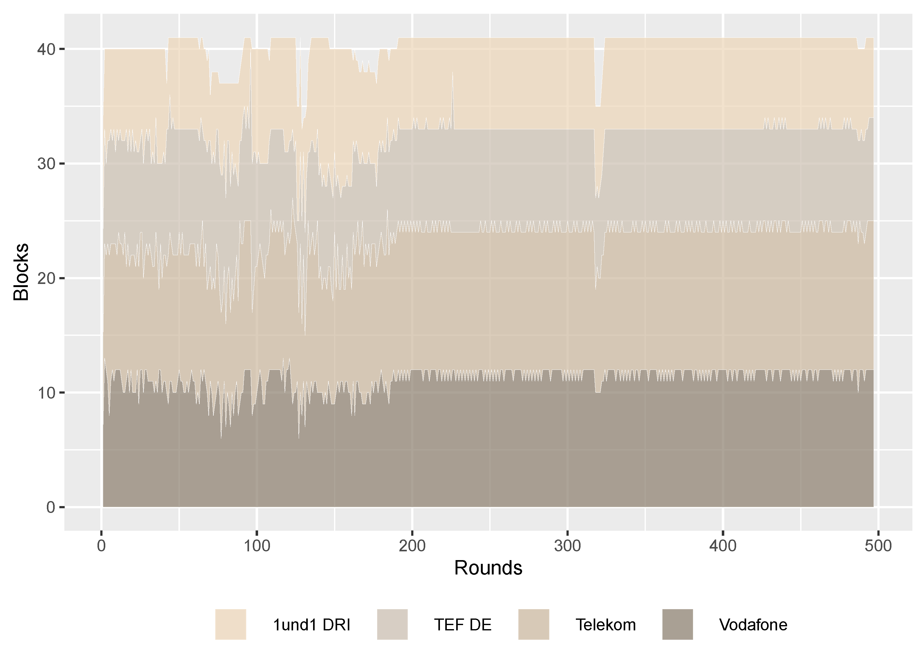
For all other frequencies, there was a serious competition by all four participants as shown in Figure 2. The structure of high bidders started out rather volatile: at first, high bidders changed often for most frequencies as did the number of blocks that an individual firm held high bids on. At the maximum in round 125, 17 blocks out of 41 changed in their current high bidder. However, once the dispute about the n1 band was all but settled in round 187, this volatility also cooled down as competition concentrated on just one block in the n78 band: after round 187, bidders changed for a total of just seven times in the 2 GHz band. In the higher band, the high bidder changed just for one block in almost every round until the very end in round 497. However, there were some rounds with more movement, especially round 318 when Telekom surrendered several blocks before securing them again later. In other instances, Telefónica attacked 1&1 and caused some short-lived changes in the bidding structure in round 325 but could not sustain outbidding its competitor and lost the blocks back to 1&1 in the following rounds. Overall, the respective companies’ amount of blocks matches expectations reasonably well. Telekom and Vodafone were successful bidding for 13 and twelve blocks, respectively. However, the overall amount of spectrum awarded was the same for both companies at 130 MHz since Vodafone won the bidding for the 20 MHz block. Telefónica was able to secure nine blocks for an overall amount of 90 MHz while 1&1 won seven blocks for 70 MHz. The difference between Telefónica and the other incumbents might come as a surprise at first glance. However, this observation can be rationalized when the fact that both Vodafone and Telekom operate more advanced networks and have to meet higher expectations by their clients is taken into account. Telefónica inherited all of E-Plus’s clients after the merger in 2014—clients that often paid less than what one would pay for Vodafone’s or Telekom’s contracts. This is also reflected by the company’s monthly ARPU (Average Return Per User) of just EUR 10.2 compared to Telekom’s EUR 12 and Vodafone’s EUR 13 as of 2019. In return, their service is often not as good and the supply with LTE is far lower than in the other two networks: While Telekom and Vodafone reach 98% and 96% of households, respectively, Telefónica only covers around 90% of the population (Telefónica Germany 2019a). Additionally, Telefónica achieved the lowest revenue among the three incumbents and thus could likely not afford to bid as high as Vodafone and Telekom. In fact, the final individual expenditure of the three incumbents amounted to EUR 2.2 billion for Telekom, EUR 1.88 billion for Vodafone and EUR 1.4 billion for Telefónica.

To be able to compare the results to the market’s anticipations and for further analysis in Section 4, ex-ante expectations are needed. The exact numbers based on a market evaluation are confidential and cannot be disclosed. However, Wirtschaftswoche (2019) refers to an analysis by the private bank Berenberg and report an estimated total revenue of the auction of roughly 3 billion Euro. As a robustness check we will conduct the analysis with an equal distribution of this amount across all bands.

4. Price Discovery

As outlined in the previous section, especially in Figure 1, the prices for the 41 frequency blocks developed slowly over time. When the firms started bidding, prices were not much higher than the required minimum bid, but they ended up being 62 times higher after 497 rounds as the four companies learned about their rivals’ intentions and valuations of the spectrum. This process of price discovery is examined in this section by conducting one unbiasedness regression for every auction round. The comparison of the results of all regressions can then reveal the increase in informativeness over the auction rounds.

4.1. Estimation

To test the noise and learning hypotheses, we conduct the unbiasedness regression as in Biais et al. (1999) (who themselves follow Hodrick (1987)). While learning itself might not be a linear process, the model here presents the best linear approximation to the potentially nonlinear learning behavior. The regression equation in its basic form which is then estimated using OLS reads as follows:

$$v_i-𝔼\left[v_i\right|I_0]={\alpha }_t+{\beta }_t(P_{i,t}-𝔼\left[v_i\right|I_0])+Z_{i,t},$$

(3)

where the index i indicates the cross-section of blocks which is exploited for estimation while the estimation is conducted once per round t. The left-hand side of the equation is the difference between the fundamental value of a frequency block, $v_i$, and its ex-ante expectation $𝔼\left[v_i\right|I_0]$. The fundamental value of each block will be proxied by the final bid in round 497. Due to the design of the auction as a simultaneous ascending auction, any competitor who still owned enough bidding rights could have placed a higher bid if they had valued the block higher. Since this did not happen and the auction ended, the final bids qualify as a proxy for the fundamental value $v_i$. The ex-ante expectation $𝔼\left[v_i\right|I_0]$ reflects the market’s expectation about the value of the prices before the auction began and thus before the bidders or the BNetzA supplied any additional information.

On the r.h.s. of Equation (3), the difference $P_{i,t}-𝔼\left[v_i\right|I_0]$ measures the return from the ex-ante expectation about the fundamental value to round t of the 5G auction. $Z_{i,t}$ is a noise component marked by heteroskedasticity. The parameter ${\beta }_t$ should be equal to zero under the noise hypothesis that was presented in Section 2.4.1. The reason for this is that under the noise hypothesis, the covariance of the two returns is equal to

$$cov\left(v_i-𝔼\left[v_i\right|I_0],P_{i,t}-𝔼\left[v_i\right|I_0]\right)=cov\left(v_i-𝔼\left[v_i\right|I_0],ϵ\right) =0$$

(4)

and thus ${\beta }_t=0$. If the prices were fully informative as stipulated by the learning hypothesis in Section 2.4.2, ${\beta }_t$ should be equal to one since the return from the ex-ante expectation to the price in round t would fully explain the final return $v_i-𝔼\left[v_i\right|I_0]$. As learning can be expected to take place gradually over the course of the auction as participants make their valuations known step by step, we expect ${\beta }_t$ to increase over time, i.e., from one auction round to the next. Since the proxy for the fundamental value is the final price that was paid in the auction, the parameter will be equal to one at the very end by construction. This does make sense, however, since the four participants had fully revealed their intentions and valuations as well as their willingness to pay by the time the auction came to a close.

For the following estimation, all values were divided by the first price. This was done in order to clean the returns from any strategic bidding that occurred in the first round. For example, 1&1 overbid every minimum bid by EUR 20 million, clearly indicating that the company was willing to compete for spectrum from the start. By taking away this signal in the first round, we normalize bids for individual blocks. This is important for the comparison of blocks since they already started out containing different levels of information depending on the participants’ behavior. Dividing by the first price makes the price discovery more comparable across different blocks since differences in the starting bids are accounted for. If the first price does not exist, the first existing price is used for this purpose as it is the first piece of information that is available for the specific frequency block. This is especially true for the single 20 MHz block in the n78 band as the first bid was not submitted until round 43 but also holds true for some other blocks that were most likely left out by chance since the participants had a limited number of bidding rights. This would explain why some blocks did not list a high bid in round one even though they were perfect substitutes for the other blocks in the respective band and the participants would have been able to spread demand more equally across all blocks. This modification of Equation (3) leads to the estimated regression

$${\displaystyle \frac{v_i-𝔼\left[v_i\right|I_0]}{P_{i,1}}={\alpha }_t^{\prime }+{\beta }_t\frac{P_{i,t}-𝔼\left[v_i\right|I_0]}{P_{i,1}}+u_{i,t},}$$

(5)

with the residual $u_{i,t}=Z_{i,t}/P_{i,1}$.

4.2. Learning during the Auction

Since there are 497 different rounds, the regression model presented in Equation (5) is estimated 496 times. The results are shown in Figure 3: As expected, the estimated parameter of the regression increases over time until it is equal to one in the final rounds of bidding. Even though the estimated effect is larger than zero already in the beginning, the noise hypothesis cannot be rejected on the 5% significance level until round 86. This could reflect the fact that the participants would try and set up a low-price equilibrium. If one looks at Figure 1, the slope of the total sum of all bids starts to increase significantly around the same time that the noise hypothesis can be rejected on the 5% significance level. In the following 357 rounds, we can observe a period of partial informativeness as ${\widehat{\beta }}_t$ is increasing but significantly different from both zero and one. The level of informativeness increases most rapidly between round 100 and round 187. This is related to the fact that price discovery is taking place in both frequency bands up until that point. Afterwards, learning almost only stems from the high band at 3.6 GHz and since the bids only increased at a very slow pace at this stage, the slope of the regression also increases more slowly from the moment on that bidders have agreed on the 2 GHz allocation. In round 443, the learning hypothesis cannot be rejected for the first time. The same holds true for most of the following 54 rounds with the exception of rounds 472 and 473. In the remaining 52 rounds, the hypothesis that the submitted bids are entirely informative cannot be rejected anymore.

Biais et al. (1999) provide an additional view on the learning process by comparing the root mean square error (RMSE, standard error of the residual) of each regression to the standard deviation of returns. They claim that if prices were not informative at all, the RMSE should be equal to the standard deviation of returns on the left-hand side of the regression in Equation (5). The reason is that, since the bids had no informational content, the model would not be able to explain the returns’ variance at all. Instead, the regression’s $R^2$ should be equal to zero. The process of learning is therefore indicated by a declining RMSE or an increasing $R^2$ over time. Following the same line of argument, the explanatory power of the regression should be perfect if the learning hypothesis was true. In turn, the RMSE should be zero and the $R^2$ should be one.

This pattern is indeed what we find as can be seen from Figure 4. At first, the standard error of the residuals is approximately equal to the standard deviation of returns, albeit a bit lower during the first 50 rounds. After approximately 100 rounds, the RMSE starts to shrink continuously to less than a third of the standard deviation of returns before decreasing steeply and almost disappearing completely by the end of the auction. The pattern of the $R^2$ is the reverse, starting close o zero, increasing by roughly 60 percentage points up to round 180 and then steadily climbing towards 1 until the end of the auction. This finding/pattern supports the hypothesis that there is a learning process taking place during the spectrum auction. The steady decrease of the residual’s standard error indicates that the amount of information that is contained in the individual bids is growing while the noise component is decreasing as more and more bids are submitted.

It should be noted that finding a perfect fit of the model in the very last round happens by construction as we use the final price of the auction as the fundamental value. The value added of our analysis is that we can illustrate the learning path and the speed of learning during the auction. In particular, we document that the auction seems to have had two parts (for the n1 and then 78 band) rather than being a uniform auction for all available frequency bands. The German 5G auction has been criticized for taking a long time. Our results (in particular the robustness checks presented below) point to a conclusion that the participants settled first on the available frequencies in the n1 band and only subsequently dug into the n78 band. Separating both auctions, thus, might have allowed to come faster to a close of the auction.

4.3. Robustness Checks and Discussion

In order to test the robustness of our findings, several robustness checks are performed. The first one consists of adding control variables such as the market share of the high bidder or whether the holder of the high bid changed in the respective round. We find that the results are not significantly changed by including these controls. The only difference is that the noise hypothesis is rejected in most rounds, even early in the auction. This results from a more volatile estimate for ${\widehat{\beta }}_t$ after the inclusion of the control variables.

Another strategy to check the results is to split the data into four different datasets. Each one only contains the high bids of one of the four participants. For each dataset, the estimation as described by Equation (5) is repeated. The results of this approach are presented in Figure 5. Splitting the data comes at the cost that the number of observations for some rounds is very limited. Since we do not observe all submitted bids unless they were the highest bids, the subsample dataset contains large gaps by construction. For this reason, some rounds have to be excluded during the estimation. This is, for example, the case for the first round of Telefónica’s campaign because the company only submitted bids for the n78 band at the minimum bid. This means that the regressor is constant for the entire round and no estimate for ${\widehat{\beta }}_t^{O_2}$ is produced. In total, two rounds had to be excluded: one for Telefónica and one for 1&1. Another limitation of this approach is that the estimate is likely to suffer from small sample bias. This is especially visible for 1&1, where the estimate ${\widehat{\beta }}_t^{1\&1}$ is extremely volatile (see Figure 5d) and is likely not reliable. To a lesser extent, the same holds true for Telefónica’s estimate for ${\widehat{\beta }}_t^{O_2}$ in early rounds. Roughly around the 187 round mark when the 2 GHz disputes were settled, the estimate becomes more consistent and closer to expectations. The other two incumbents’ estimates ${\widehat{\beta }}_t^{Telekom}$ and ${\widehat{\beta }}_t^{Vodafone}$ are easier to compute due to the relatively larger availability of observations since these two companies bid for more spectrum over the course of most of the auction. It comes as no surprise that these estimates are more precise and follow expectations more closely. In fact, the noise hypothesis cannot be rejected for Vodafone or Telekom in most of the first 187 rounds. In some of these rounds, the hypothesis can be rejected but it is also possible that this stems from the small number of observations that are available. For both cases, the informativeness of prices increases as the auction goes on. The larger volatility of the estimates can be attributed to rounds where the respective companies lost their high bids on one or more blocks. The learning hypothesis for Vodafone cannot be rejected anymore after round 246 after a previous phase of informativeness is interrupted for several rounds. The results for Telekom are more comparable to the overall estimation. However, it holds true for both estimates that the standard errors are much larger, leading to larger periods in which the two individual hypotheses cannot be rejected on the 5% significance level. Overall, the findings of the previous section still seem to be robust to splitting the sample up among the individual participants even though the low number of observations makes this estimation a lot less reliable. It would be interesting to test this with a complete dataset for every bidder in the auction in the future.

In a similar approach to the previous test, the two frequency bands were analyzed independently. The results are presented in Figure 6. As can be seen from Panel (a), the estimate is highly volatile for the n1 band. It starts out significantly negative before overshooting to the opposite extreme, being significantly larger than one. An important takeaway, however, is the fact that the learning hypothesis cannot be rejected from round 178 onward. Competitive bidding in this band stopped 9 rounds later. The estimate for the n78 band shows a more recognizable learning pattern, increasing for most of the auction. However, the estimate is both lower than zero and larger than one at several points during the auction. In this setting, the noise hypothesis cannot be rejected until round 171. The learning hypothesis cannot be rejected from round 182 on, even though competition continued until the end of the auction. This is due to the high standard errors of the estimate which likely result from the lower number of observations that are available for each individual band.

Splitting the data by frequency band reveals that learning in the lower n1 band was substantially faster than in the n78 band. While the auction had been designed to sell both bands together, it seems that the auction participants still regarded the two bands as being different. The fact that the n1 band part of the auction came to an informational close already very early might indicate that the value was more obvious, probably due to the fact that this band is used for 4G standard. Also, learning really only started significantly in the n78 band after the n1 band was more or less settled. This leads us to conclude that the companies focused on the bands sequentially which might have allowed to split the auction in two separate auctions for each band.

As a fourth test, the normalization of returns using the first price was dropped. Instead, log returns were used to compute the estimates. This means that the regression equation changed to:

$$log\left(v\right)-log\left(𝔼\left[v\right|I_0]\right)=a_t+\beta \left(log\left(P_t\right)-log\left(𝔼\left[v\right|I_0]\right)\right)+e_t.$$

(6)

If the previous result of a learning pattern was robust, this more conventional method should yield comparable results. In fact, the learning curve is similar when using log returns. However, the prices start out being partially informative already in round one. The noise hypothesis is rejected in every single round but so is the learning hypothesis apart from the very last rounds. This is due to the comparably small standard errors on the estimate when using log returns causing the confidence intervals to become smaller and smaller such that the learning hypothesis is rejected even when the level of informativeness increases. However, this finding can also be backed by theory: since prices were still increasing in every auction round, the learning hypothesis that prices are fully informative should not be true until the very end of the auction. Also since the first round strategies are not excluded here, the informativeness is higher from the start. However, this test’s results are in line with what has been presented before and support the existence of a learning pattern. Furthermore, information contained in prices also increases much faster in the opening phase when bids for all 41 blocks are increased compared to the phase after the 2 GHz band had already been split among the participants. The results from using log prices are displayed in Figure 7.

5. Conclusions

This article examines the process of price discovery and learning from competitors’ bids in the 2019 German 5G auction. The amount of information that was contained in the submitted bids was very low at first. This means that the noise hypothesis which states that submitted bids are not more informative than ex ante expectations, cannot be rejected until the 86th round of the spectrum auction. Thereafter, the slope of the unbiasedness regression increases, indicating an increase in informativeness, albeit bids are still only partially informative. The speed of learning picked up at the end of the auction when the BNetzA decided to increase the minimum increment to EUR 13 million. This uncovered the companies’ private information at a faster rate, indicated by a steep increase of the estimates from one auction round to the next. Starting in round 443, the hypothesis that submitted bids are entirely informative cannot be rejected anymore. From this moment on (with small interruptions), the estimate is not significantly different from 1.

Our results indeed support the notion of a Walrasian tâtonnement process: Companies places bids tentatively at first, probably observing their competitors bidding behavior. This makes sense as with 1&1, there was a new competitor at the bidding table. The informativeness of bids then starts to increase, but it still took 497 rounds for the auction to come to an end. As bidders gradually made their true valuation of the spectrum know, maximum bids for each block became more informative. A consensus price seems to be reached faster in the established n1 band than in the new n78 band. Indeed, our results allow the conclusion that the companies focused on the n1 band first and then turned to the n78 band. Hence, to save time, conducting separate auctions for the two bands might have been better. Overall, the auction gradually revealed preferences in line with the auction setup. Learning occurred steadily so that we conclude that the auction was an efficient mechanism to allocate the 5G spectrum.