Abstract
This paper studies the relationship between natural disasters and economic growth in the disaster-prone country of Iran, using a spatial Durbin panel model and covering the time period from 2010 to 2016 and including 29 provinces. The results of the empirical investigation suggest that there is a statistically significant positive relationship between the spatially-lagged occurrence of natural disasters and the change of the first difference of the natural logarithm of GDP per capita. Moreover, the estimations support the findings of previous cross-country studies, namely that we cannot find empirical evidence for a statistically significant direct effect of natural disasters on economic growth in the short term. When including time-lags, we can see a statistically significant positive effect of natural disasters on economic growth after two years. When taking into account the disaster type, which is mainly earthquake and flood in the case of Iran, the results suggest that the positive spillover effects are, rather, driven by earthquakes, and that there is a direct positive effect of floods in the short run. These findings extend existing literature and add new insights that are not just relevant for the case of Iran. The novelty of this study is that established and innovative approaches are used to study natural disasters on the provincial level, instead of the country level, and also take into account spatial spillover effects after disaster events that have been rarely discussed in literature.
1. Introduction
Extreme weather phenomena and other natural disasters, which have been attributed to climate change, are dominating the political and public discourse recently again. However, the devastating impact of natural disasters is more likely to afflict people in developing countries, with those in low-income and middle-income countries more vulnerable to the highest disaster risk (World Risk Report 2017). Therefore, we will focus on the case of Iran, as it is an interesting case study in this context. The country is located in the Middle East and North Africa (MENA) region which has experienced many natural disasters over the past thirty years, affecting more than 40 million people and costing their economies about US$20 billion (World Bank 2014). Main disaster events in the region are floods, earthquakes, storms and droughts, with Iran being the most affected country. In April 2019, Iran experienced the most severe flood ever recorded in the MENA region, affecting more than 10 million people and causing damage of more than US$2.5 billion. Furthermore, over the past 30 years two of the most-deadly earthquakes of modern times hit Iran which killed combined more than 65,000 people and caused damage of almost US$9 billion (Emergency Events Database 2020).
This paper’s research question is two-fold, because on the one hand, we want to study the relationship between natural disasters and economic growth in a disaster-prone country using provincial data, and on the other hand, we want to find out if there are post-disaster spillover effects from neighboring provinces. This study uses a balanced panel of 29 Iranian provinces for the time period 1389 to 1395 according to the Iranian calendar years, which is approximately 2010–2016. As an econometric approach, it uses the spatial Durbin panel model with the maximum likelihood estimation. The contribution of this study is three-fold. First, there has not been a case study of Iran that has systematically studied the effect of natural disasters on the economic performance of the country. Second, previous studies on natural disasters and economic growth have mainly focused on the cross-country level, but here we will use a case study of Iran with cross-provincial data. Third, spatial aspects have rarely been included in previous regression models of the literature on natural disasters and economic growth.
Furthermore, this study ties on the first comprehensive study on the political economy of natural disasters (Albala-Bertrand 1993), while using an innovative methodology and latest available data. It covers the fields of macroeconomics, economic growth, development economics, and environmental economics, that are mentioned under the scopes of the Journal of Risk and Financial Management (JRFM). The aims and scopes of this study and the journal show further overlapping, as the interest is to study the economic impact of different types of natural disasters, while also discussing the natural disaster risk as well as challenges and opportunities for decision makers related to disaster prevention and relief. Therefore, it is an important contribution to the special issue on the political economy of natural disasters.
2. Literature Review
In the natural disaster literature, we can find several approaches that try to uncover the link between natural disasters and economic development with inconclusive results. There are different hypotheses and theories on how an economy reacts in the short and long run after the impact of a natural disaster event. On the one hand, when a natural event turns into a disaster, it might cause the loss of human life and destroy infrastructure, which means a loss of human and physical capital. This might affect economic performance in a negative way. On the other hand, several authors find support for the creative destruction argument which means that after the destruction, there is the opportunity to replace old infrastructure and technology with newer versions.
One of the first comprehensive studies on the political economy of natural disasters comes from Albala-Bertrand (1993) who introduces an analytical framework and a macroeconomic model which shows the disaster’s effects on output. Moreover, he empirically analyses the relationship between natural disasters and several macroeconomic variables of 28 developing countries. His results suggest that the average growth rates increased in all cases after the disaster and the effects disappear in the long run. In addition, Skidmore and Toya (2002) show with the help of the Cobb–Douglas production function that GDP does not account for damage to capital and durable goods in the short run, but the addition of new capital in the immediate term may increase GDP. They hypothesize that this growth is due to capital stock accumulation, human capital accumulation, or improvements in technological capacity. Despite the destruction of capital, disasters increase the return to human capital relative to investment capital and increase total factor productivity through the adoption of newer and more productive technologies.
Furthermore, Klomp (2016) summarizes more traditional neo-classical growth models, like the Solow model and Schumpeter’s creative destruction theory. The former predicts that the reduction of the capital–labor ratio drives countries temporarily away from their long-run growth path, while the endogenous growth models provide less clear-cut predictions. The latter may even predict higher growth rates as a result of natural disasters since these shocks can work as an accelerator for upgrading the destroyed capital stock. In contrast, Kellenberg and Mobarak (2008, 2011) argue that the benefits of investing in more technologically advanced capital are offset by the short-run productivity losses of a disaster because extra time is required to train workers and to fully incorporate new technology.
The same authors argue in favor of an inverted u-shape relationship between natural disaster damage (measured by deaths) and the level of economic development, meaning that in the early stages of economic development, countries will not put high priority in disaster prevention, but instead will use production methods that increase the vulnerability to disasters. Therefore, there is a positive relationship between economic growth and disaster deaths until a turning point. After this peak, the awareness for disasters becomes higher and the potential capital loss will be higher, so it becomes more attractive to invest in disaster prevention and disaster-proof infrastructure. This will lower the death rates. However, their empirical results also show that this relationship can only be found for landslides, windstorms, and floods. For earthquakes and heat waves, they find a negative relationship between disaster deaths and per capita GDP. Another study by Schumacher and Strobl (2011) argues that the relationship depends on the risk level of the geographical region. More precisely, they expect that low-risk countries have an inverted u-shaped relationship and high-risk countries have a u-shaped relationship.
Other studies focus on the effect of the disaster impact over time and possible moderating factors: first, Barone and Mocetti (2014) show different effects in the short and long run in different regions, depending on the quality of institutions. Second, Felbermayr and Gröschl (2014) show negative effects of disasters on growth, while trade openness and institutions are moderating factors. Further evidence of negative effects is provided by Klomp (2016) who additionally look into the long-term effects of different kinds of disasters and finds that the significant negative effect of natural disasters disappear after two years for all types, except for geophysical disasters. A study by Noy (2009) focuses on the short-term effects of natural hazards on the macroeconomy. He shows that countries with a higher literacy rate, better institutions, higher per capita income, higher degree of openness to trade, and higher levels of government spending are better able to withstand the initial disaster shock and prevent further spillovers into the macroeconomy.
Overall, previous research shows that positive or negative effects of natural disasters depend on the institutional development, the disaster type, and the geographical region where the disaster event happened (Kellenberg and Mobarak 2008; Loayza et al. 2012; Klomp 2016). However, there is also a path of literature that does not find direct statistically significant effects of natural disasters on economic growth. One of these studies comes from Cavallo et al. (2013) who use the synthetic control method to examine the average causal impact of catastrophic natural disasters on economic growth. They find that only two extremely large disasters have a negative effect on output in both the short and the long runs, but these cases were followed by radical political revolutions. After controlling for these, even extremely large disasters do not display any significant effect on economic growth. One of these examples is the Iranian Islamic Revolution which occurred right after the 1978 Tabas earthquake.
The role of natural disasters in the MENA region or specifically Iran has not been intensively studied from the perspective of social sciences and economics. The majority of studies on the case of Iran are related to health aspects, geography, engineering, and natural disaster management. The first empirical studies on natural disasters and its effects on GDP per capita, savings, and investments in Iran come from Sadeghi and Emamgholipour (2008), Sadeghi et al. (2009), and Yavari and Emamgholipour (2010). Using time-series data over the period 1959–2004, the former found a negative impact of natural disasters on Iran’s GDP in the short and long run. Furthermore, they found evidence for a u-shaped relationship between natural disaster damage and non-oil GDP. In another study, Sadeghi et al. (2009) show similar results for the period 1978–2004, namely negative effects of natural disasters on per capita investment and per capita GDP in the short and long run. Finally, Yavari and Emamgholipour (2010) focus on the impact of natural disasters on total savings in the time period 1973–2006. Their results suggest that natural disasters raise the average propensity to savings in Iran.
A study by Hosseini et al. (2013) investigates the socioeconomic aspects of two major earthquakes in Iran, namely the 1990 Manjil-Rudbar earthquake and the 2003 Bam earthquake. The authors analyze different laws and policies related to disaster management as well as the social situation in the affected areas, the destruction in the affected areas, and the psychological effects of the earthquakes. Overall, they show the huge destruction and the variety of negative effects on the social and regional level. In a case study comparison including Iran, Yuan et al. (2018) show how earthquakes can facilitate civil society engagement in developing countries. Overall, their results suggest that civil society engagement experienced a sharp spike directly after the disaster event, but after several months most of the helpers disappear. The study also discusses the reactions of the governments and challenges in coordination between involved agents.
Ainehvand et al. (2019) also focus on disaster management aspects and study the challenges related to food security using semi-structured interviews of 29 experts. According to these, natural disasters have negative impacts on various dimensions of food security such as food availability, food access, food utilization, and sustainability of each of these components. The authors identified several challenges for food supply in the context of disaster relief such as geographic and weather conditions, climate change, vulnerability of people, structure and inefficiencies of disaster management, passive responses, compensation mechanisms, ineligible distribution of food assistance, organization-based responses, unsolicited donations, as well as nutrition and health considerations.
In the wider sense, there are also a couple of studies on natural and man-made hazards such environmental degradation or climate change. Farzanegan and Markwardt (2018) as well as Gholipour and Farzanegan (2018) focus on the role of institutional quality related to air pollution and environmental protection in the Middle East. The former find evidence that improvements in the democratic development of the MENA countries help to mitigate environmental problems, while the latter show that government expenditures on environmental protection alone do not play a significant role in contributing to better environmental quality. However, improvements in quality of governance are shaping the final environmental effects of government expenditures on environmental protection in the MENA region.
An overview about effects of climate change on Iran and five projections of possible future developments are presented by Ashraf Vaghefi et al. (2019) who found that compared to the period of 1980–2004, in the period of 2025–2049 Iran is likely to experience more extended periods of extreme maximum temperatures in the southern part of the country, more extended periods of extreme weather events, including dry and wet conditions. Overall, their projections show a climate of extended dry periods interrupted by intermittent heavy rainfalls, which is a recipe for increasing the chances of floods. Climate change in Iran has already had social and economic consequences such as inter-province migration (Shiva and Molana 2018) and increasing housing and residential land prices (Farzanegan et al. 2020). The former authors study climate change-induced inter-province migration in Iran from 1996–2011 and found that a rise in temperature and a drop in precipitation act as significant push factors for migration. The latter examined the effect of drought on housing and residential land prices in Iran, using panel data from 2006–2015 on the province level. According to their results, an increase in the balance of water (reducing the severity of drought) within provinces has a positive effect on property prices.
Last but not least, there has been a focus on the spatial spillover effects of natural disasters in recent years. First, Felbermayr et al. (2018) use spatial econometric panel methods and data from 1992–2013 to study the spillover effects after natural disasters that are affecting economic activities. They find, in particular, evidence for weather shocks, and substantial heterogeneity across income groups and regions. Second, Lenzen et al. (2019) analyze the economic damage and spillovers from a tropical cyclone using the case study of Australia. Their results show how industries and regions that were not directly affected by storm and flood damage suffered significant job and income losses throughout upstream supply chains. Third, Barbosa and Lima (2019) study the case of flash floods in Brazil using a difference-in-differences model and show that municipalities directly affected by a flood suffered an 8.47% decrease in GDP per capita on the year of the disaster, and that there are significant spillovers to neighboring regions.
Moreover, a case study from Thailand comes from Noy et al. (2021) who use a difference-in-difference approach with panel data of repeated waves of the Thai Household Socio-Economic Survey and satellite data to analyze the impacts of the 2011 flood across different socioeconomic groups. From the survey, they identified those who experienced the flood and those who did not. Thus, the authors could measure the direct and indirect impacts of the disaster on income, expenditures, assets, debt and savings levels for spillover households. Their results show that business income drove the negative impacts on flooded households relative to the control group. Moreover, they found spillover effects on households that were not directly affected by the flood, but are almost as large as the loss experienced by directly impacted households. Their results suggest that these spillover effects are mainly driven by declines in business income, but also by declines in wage income. This decline in business income is mostly associated with higher-wealth households, while lower-wealth households did experience a significant decline in agricultural income.
3. Data and Methodology
Unlike previous studies, this contribution will focus on natural disasters in Iran using several spatial panel models and data at the provincial level. The main argument for this approach is that the effect on the country level might be small, except for very small countries or island states, as Albala-Bertrand (1993) and other authors show for the effect of natural disasters on GDP. In the case of Iran, we would expect that even large-scale natural disasters that affect only one province or a low densely populated province will hardly be measurable in the national GDP of Iran. Therefore, we need to study the effect of natural disasters on the provincial levels. This gives us also the possibility to keep factors constant that affected all Iranian provinces at the same time and affected the national GDP, for example the Iran-Iraq War, the Islamic Revolution, and the recent economic sanctions. Within the time period of this study, the USA and European Union (EU) introduced extended sanctions against the Iranian oil trade and financial sector in 2011/2012, which affected the Iranian economy heavily in the following years. In a cross-country or time-series comparison, we will not know if the effects on GDP come from a natural disaster or from one of these major events. This problem became visible in the study of Cavallo et al. (2013).
Data for many macro-economic indicators for 31 Iranian provinces are available for the time period from 1379 to 1398 at the Ministry of Economic and Financial Affairs (MEFA). However, not all data series are available for the whole time period. Additionally, there have been several reforms related to provincial borders, for example the province Alborz that was created in 1389 and was previously part of the province of Tehran. Another example is the former province of Khorasan which was split into the three provinces North Khorasan, Razavi Khorasan, and South Khorasan in 1383. With regard to the balanced panel dataset required, the number of years and provinces in the dataset will be reduced. This leaves us with the time period 1389–1395 and 29 provinces with 203 observations. In comparison, using all 31 provinces will only provide us with a balanced panel dataset from 1391–1394 with 124 observations. As the data sources are several Iranian organizations, such as the Central Bank of Iran (CBI), Ministry of Economic and Financial Affairs (MEFA), and Statistical Center of Iran (SCI), this study will use Iranian years. The Iranian calendar has 12 months and starts in the year 622 CE of the Gregorian calendar, with the new year occurring at the beginning of spring, which is around 21 March. That means the used time period in this study is 21 March 2010 to 20 March 2017, or approximately 2010 to 2016.
Natural disaster data comes from the International Disaster Database (EM-DAT) of the Centre for Research on the Epidemiology of Disasters (CRED) at the Université catholique de Louvain. It includes a list of 234 natural disasters that took place in Iran between 1900 and 2019, causing more than 160,000 deaths and an estimated damage of more than US$27 billion. The majority of events were earthquakes and floods. The database counts 126 disastrous earthquakes with more than 150,000 deaths and an estimated damage of US$12.6 billion, and 84 disastrous floods with more than 8000 deaths and an estimated damage of US$11.5 billion. These are not all floods or earthquakes that happened in Iran during the time period, but only those classified as natural disasters by EM-DAT. In a formal definition, the database defines disasters as “a situation or event which overwhelms local capacity, necessitating a request to the national or international level for external assistance, or is recognised as such by a multilateral agency or by at least two sources, such as national, regional or international assistance groups and the media” (Below 2006). An event must fulfill following requirements to be included in the database: 10 or more people reported killed and/or 100 or more people reported affected and/or call for international assistance/declaration of a state of emergency. Figure 1 gives an overview of the spatial distribution of the occurrence of natural disasters in Iran.
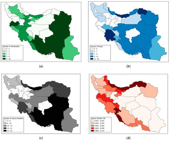
Figure 1.
Spatial distribution of the occurrence of natural disasters in Iran: (a) number of disastrous earthquakes per Iranian province, 1950–2019; (b) number of disastrous floods per Iranian province, 1950–2019; (c) number of natural disasters per Iranian province, 1950–2019; (d) natural disasters per year per 10,000 km2 (based on the years 1950–2019). Source: author’s illustration with data from International Disaster Database (EM-DAT 2020).
Since the database also includes information about the location (coordinates or names of affected cities) and the exact date of each disaster event, it is possible to create a panel for Iranian provinces using Iranian years. Two problems arise in this context. First, it is difficult to calculate the number of deaths, the number of affected people or the amount of damage for each province, if several provinces were affected by the same disasters. This issue is solved by using dummy variables as a measurement of the disasters. Second, there might be no effect of the disaster reflected in the outcome variable, if a disaster happened at the end of a year. To solve this issue, the natural disaster dummy variable is 1 when a disaster happened six months before and 0 if no disaster happened six months ago. The models were also estimated without the six months delayed dummy variables and it did not affect the results in a meaningful way. According to the available data, there were 21 disaster events (13 earthquakes, 7 floods, and a storm) in the time period 1389–1395, affecting 18 of the 29 provinces. The deadliest event was the 1391 earthquake in the province of East Azerbaijan, killing 306 people and affecting more than 60,000 people. The most severe flood during this time period happened in 1393 in the north east of Iran, killing 37 people and affecting approximately 440,000 people in six provinces.
The following Table 1 gives an overview of the variables that are used in the estimations. A detailed list of variable definitions can be found in Table A1 of Appendix A. In addition, all variables have been tested for unit roots, and the results of several tests are also reported in Appendix A, namely in Table A2.

Table 1.
Summary statistics of used variables.
Using the described data, this study applies the spatial Durbin panel model (SDM) which is a further development of the spatial Durbin model using cross-sectional data introduced by Anselin (1988). It has the following structure, as presented by Elhorst (2014, pp. 7–10):
where Y denotes an N × 1 vector consisting of one observation on the dependent variable for every unit in the sample, α is the constant term, X denotes an N × K matrix of exogenous explanatory variables, β is an associated K × 1 vector with unknown parameters to be estimated, and ε is a vector of disturbance terms. Moreover, δ is called the spatial autoregressive coefficient, while θ, just as β, represents a K × 1 vector of fixed but unknown parameters to be estimated. W is a non-negative N × N matrix describing the spatial configuration or arrangement of the units in the sample. This model includes a spatial lag of the dependent variable WY and a spatial lag of the explanatory variable WX, therefore it combines the spatial autoregressive (SAR) model and the spatial lag of X (SLX) model.
LeSage and Pace (2009, pp. 25–31) summarize several motivations for including spatial autoregressive processes in the regression models. First, the authors refer to the time-dependence motivation which means in the case of this study that the development in an Iranian province might depend on the development of neighboring provinces in previous time periods, for example when determining tax rates or other local policies which might be based on the experience of neighboring provinces. Although the tax rates were set over time by the cross-section of provinces representing our sample, the observed cross-sectional tax rates would exhibit a pattern of spatial dependence. This situation would suggest to use a SAR model. Second, the authors argue for an omitted variable motivation which means that our model might not include important explanatory variables related to geographical location that may exert an influence on our dependent variable. They mention examples such as unobservable factors including location amenities, highway accessibility, or neighborhood prestige, and argue that it is unlikely that explanatory variables are readily available to capture these types of latent influence. Here, we should use the SAR, SLX or SDM models, because they capture such influences from neighboring provinces. The third motivation mentioned by the authors is the spatial heterogeneity motivation which assumes that in our panel dataset the intercept for each province can be treated as a spatially structured random effect vector. Making an assumption that observational units in close proximity should exhibit effects levels that are similar to those from neighboring provinces provides one way of modeling spatial heterogeneity. Here, the dependence can be viewed as error dependence, and with this assumption we should use the spatial error model (SEM) or spatial Durbin error model (SDEM).
A fourth argument is the externalities-based motivation which can be both positive and negative in the spatial context. These externalities arise from neighboring provinces and can have sensory impacts, for instance in the case of pollution and environmental degradation. The latter might also cause the loss of habitat for humans and animals, possibly due to lack of water and food availability, and this might affect migration to neighboring provinces. In contrast, a beautiful landscape and availability of jobs might also make neighboring provinces more attractive. Here, we can use the SLX and SDM models, because these can model the spatial average of neighboring province characteristics that might affect our dependent variable. Finally, LeSage and Pace (2009) also highlight the model-uncertainty motivation, meaning uncertainty regarding the type of model to employ as well as the conventional parameter uncertainty and uncertainty regarding specification of the appropriate explanatory variables. The authors compare the SAR and SEM models and argue in favor of the SDM model, which includes spatial lags of dependent and explanatory variables, in the case of uncertainty. In this example, we have uncertainty regarding the presence of spatial dependence in the dependent variable versus the disturbances.
While taking into account the discussed arguments, the most adequate model for this study is the spatial Durbin panel model (SDM), because it will capture the spillover effects of natural disasters from neighboring Iranian provinces that are expected to affect the economic performance. In addition to the theoretical discussion, we have also used likelihood ratio (LR) tests to compare different spatial panel models. The results presented in Table A3 of Appendix A support the selection of SDM, because it shows the better fit compared to other models with fewer explanatory variables. Furthermore, spatial characteristics of the used data series have been tested using Moran’s I and Geary’s C. According to the results reported in Table A4 of Appendix A, several of the used variables show spatial autocorrelation, namely the disaster dummy, the natural logarithm of GDP per capita and its first differences, as well as the variables trade and foreign direct investment inflows. These results provide evidence for spatial patterns in the data series and, therefore, support the argument for the usage of spatial models. For the tests of spatial autocorrelation and the spatial models in this study, we have used a row-standardized spatial weights matrix W based on contiguity which reflects neighboring provinces of first order. It was created based on the political borders of Iran that have existed since the Iranian year 1390 (2011). The spatial contiguity matrix W* is a binary 29 × 29 matrix the entries of which, , are 0 or 1. An entry is equal to one if the provinces i and j are neighbors and 0 otherwise. This can be noted in the following way:
We calculate the row-standardized spatial weights matrix W by dividing each matrix entry by the sum of its row:
A row-standardized matrix has several advantages, for example the coefficient for spatial autocorrelation Moran’s I will range from −1 to 1. Moreover, we can interpret the spatial lag of a variable in a specific time period as the average of neighboring provinces in this time period (Anselin 1988, pp. 17–29; Elhorst 2014, pp. 12–13).
Based on existing literature on the topic and described assumptions related to spatial autocorrelation, this study formulates three hypotheses with the focus on the case of Iran:
Hypothesis 1.
Spatial spillover effects of natural disasters from neighboring provinces are associated with positive economic growth in a province in the short and intermediate term.
Hypothesis 2.
There is a negative statistically significant direct effect of natural disasters on economic growth in the short and intermediate term.
Hypothesis 3.
The direct effects and indirect spillover effects of natural disasters on economic growth depend on the disaster type.
These hypotheses focus on spatial and temporal characteristics of natural disasters and its interaction with economic performance that have been comprehensively or briefly discussed in previous studies. First, spatial spillover effects of natural disasters are mainly associated with negative impacts on neighboring regions, such as significant job and income losses (Lenzen et al. 2019) and negative effects on GDP growth (Barbosa and Lima 2019). However, there is also empirical evidence for heterogeneous effects on economic activities measured by night-time light (Felbermayr et al. 2018). The authors found an increase in economic activities due to spatial spillover effects of natural disasters for precipitation and cold related disasters, and negative spillover effects for droughts, using the global sample. This also applies in the case of low income group countries as well as the sub group Central Asia and MENA. Therefore, we expect a positive association between spillover effects from natural disasters and economic performance in Iranian provinces.
Second, the case studies from Iran that are related to natural disasters and economic growth are limited and the existing studies such as Sadeghi and Emamgholipour (2008), Sadeghi et al. (2009), and Yavari and Emamgholipour (2010) only use time series data on the country level with very few observations and control variables. They provide evidence for negative direct effects of natural disasters on GDP per capita in the short and long runs. Other cross-country studies have shown that the effects are heterogeneous and depend on different country characteristics, such as institutional development, level of economic development and geographical location (Noy 2009; Loayza et al. 2012; Barone and Mocetti 2014; Felbermayr and Gröschl 2014; Felbermayr et al. 2018). After the initial shock of the disaster, there is evidence for many cases that there will be a negative effect on the economy, but this effect disappears after only a few years. However, results are different depending on the type and strength of the disaster. Overall, we can summarize that there will be different reconstruction and development paths after the disaster, as seen in Klomp (2016) and Chhibber and Laajaj (2008), and thus the expected effect is not clear.
Third, previous studies have shown that the disaster type matters (Loayza et al. 2012; Felbermayr and Gröschl 2014; Klomp 2016; Felbermayr et al. 2018), therefore we are interested to study its impact for the case of Iran. As we are dealing only with earthquakes and floods in this study, we can have a look at the possible effects in previous studies. Loayza et al. (2012) found a positive and statistically significant effect of floods on GDP growth, while earthquakes show a negative effect, but in most specifications it is not statistically significant. Moreover, Klomp (2016) shows that there is a statistically significant direct negative effect of geophysical disasters as well as meteorological and hydrological disasters on economic growth in the short term. However, this effect disappears after two years for all types, except for geophysical disasters, even in the case of large-scale disasters. According to Felbermayr and Gröschl (2014) the effects of earthquakes and precipitation are statistically significant and negative. This is also supported by Felbermayr et al. (2018) who study weather-related disasters and found in their full sample and low-income countries sample that precipitation has a statistically significant negative effect on GDP growth, although the effect becomes positive one year later. When focusing on different regions, this result could be confirmed in the case of Latin America, while the effect one year later becomes insignificant for South East Asia. In the case of Central Asia and MENA, the effect will be statistically significant and negative in the same year and the year after. Overall, the expected effect is not clear.
The empirical specification for this study is based on Loayza et al. (2012), Felbermayr and Gröschl (2014), Klomp (2016), and Felbermayr et al. (2018), who use worldwide samples to study similar relationships. With the following spatial Durbin panel model, we want to test our hypotheses, using maximum likelihood estimation (MLE) and panel data from 1389 to 1395 (2010–2016) for 29 Iranian provinces:
Here, the dependent variable is the first difference of the natural logarithm of the gross domestic product (GDP) per capita. Its spatial lag of first order with the coefficient δ is also included in the model, which is calculated with the help of the spatial weights matrix W. It captures the spillover effects from economic growth coming from neighboring provinces. The subscript i represents the Iranian provinces, the subscript t represents the Iranian years, and the subscript j refers to the neighboring Iranian provinces of first order. In addition, the model includes a constant α and an error term ε, and the term Disaster represents the dummy which takes the value 1, if a natural disaster took place six months ago, and 0, if not. This dummy is replaced with dummies for earthquake and flood events in some of the estimations.
Since we are using a spatial Durbin panel model, we will include both the spatial lags of the dependent variable (with coefficient δ) and the independent variables (with coefficients θ) in the model. The latter includes not just the disaster dummy and its spatial lag, but also a set of control variables, labelled Controls, and its spatial lags. These variables are the natural logarithm of population size, the consumer price index (CPI) with base year 1395 (2016), the expenditures of provincial governmental organizations and the province’s acquisition of capital assets as a percent of GDP, the foreign direct investment (FDI) inflows as a percent of GDP, the trade volume as a percent of GDP, and one-year lagged natural logarithm of GDP per capita. These established predictors of economic growth are also used in the aforementioned benchmark models. In addition, some of the specifications will include time lags of the dummies for natural disasters, earthquakes, and floods, as well as its spatial lags. For a first glimpse at relationships between used variables, Appendix A includes Table A5 with a correlation matrix.
Furthermore, the model uses province fixed-effects π and controls for time-specific effects ω using dummy variables for each year. After applying the Hausman test, the fixed-effects model was chosen. Province fixed-effects are used to control for individual factors that affect each province over the whole time period, for example culture or religion. In the case of Iran, the predominant religion is Islam although despite this homogeneity, it is a multi-ethnic country. Beyond the ethnic majority group of Persians, there are several ethnic minorities, including Azeris, Kurds, Lurs, Bakhtiaris, and Beluchis, each with their different local languages and cultural traditions. These ethnic groups are concentrated in different provinces, which are sometimes even named after these groups.
4. Results and Discussion
Post-disaster spillover effects from neighboring provinces show a statistically significant positive association on conventional levels with the first difference of GDP per capita in all nine specifications of Table 2. More precisely, the coefficient of W * Disaster ranges from 0.069 to 0.095, thus suggesting an average increase of GDP per capita between 6.9% to 9.5% due to the appearance of natural disasters in neighboring provinces in the year of the disaster events. Adding temporal lags of one and two years show that the effect disappears after one year, and therefore we can interpret it as short-term positive externalities from neighboring provinces. These results are also supported by other types of spatial panel models that are reported in Table A6 and Table A7 of Appendix A. These positive spillover effects support several findings of Felbermayr et al. (2018) who use a worldwide sample of grid-based night-time light emission data as well as meteorological and geological data. They found similar positive spillovers on growth for precipitation in the global sample, low-income countries, and MENA countries, using different specifications. For wind, their results are mixed. This also applies for spatial spillover effects that are lagged by one year. Earthquake disasters are not included in their study.
Table 2.
Results of spatial Durbin panel model (SDM) using maximum likelihood estimations (MLEs, with natural disaster dummy variable).
The increase in economic growth can be explained by a sudden increase in demand in the construction sector and a boost in employment. In addition, businesses and laborers might leave the disaster-affected provinces temporarily or completely and move to neighboring provinces, which would increase economic activity as a result. Furthermore, the natural disaster events might destroy or interrupt businesses and production sites, which are the competition of neighboring provinces, causing a higher demand for products and services from the neighboring provinces, which might also create new jobs. To support these arguments, we can find evidence in previous studies. First, Hosseini et al. (2013) show that during the reconstruction processes of large earthquakes in Iran, the emphasis was put on reconstruction of residential buildings and not on commercial buildings. Therefore, some non-essential sectors will temporarily be unavailable in the disaster-affected parts of the province.
Second, Shiva and Molana (2018) study climate change induced inter-province migration in Iran from 1996–2011 and found that a rise in temperature and a drop in precipitation act as significant push factors for migration. However, they focus instead on climate change-related disasters and not the disasters discussed in this study, thus giving only little evidence and support for our arguments. Third, Pavel et al. (2018) study internal migration in Bangladesh resulting from floods, cyclones, and riverbank erosion, thus providing more evidence for people’s behavior after natural hazards and related migration dynamics. Their findings suggest that transient shocks (floods and cyclones) induce households to move to nearby cities, sometimes temporarily, while permanent shocks (coastal erosion) push people to big cities with more opportunities. In general, this supports our previous arguments. Overall, the findings of positive spillover effects from natural disasters on economic growth support our Hypothesis 1.
Contrary to existing literature on the case of Iran (Sadeghi and Emamgholipour 2008; Sadeghi et al. 2009; Yavari and Emamgholipour 2010), we cannot find evidence for a statistically significant direct negative effect of natural disasters on the economic performance in the year of the disaster event. However, the two-year lagged disaster dummy shows a positive relationship that is statistically significant on the 5% level. The coefficient suggests that GDP per capita increases on average by 4% two years after the disaster event. These results are also supported by other types of spatial panel models that are reported in Table A6 and Table A7 of the Appendix A, which not only include the commonly used spatial models as presented in Elhorst (2014), but also report the results of different estimation techniques such as maximum likelihood estimation (MLE) and ordinary least squares (OLS). A statistically significant positive or non-significant direct effect of natural disasters on economic growth is not a surprising result, as it has been found in previous studies such as Albala-Bertrand (1993) for 28 developing countries, Cavallo et al. (2013) for 196 countries, Loayza et al. (2012) for 68 developing and 26 Organization for Economic Cooperation and Development (OECD) countries, Felbermayr and Gröschl (2014) for 108 countries, and Felbermayr et al. (2018) for 24,000 grid cells.
Moreover, Felbermayr and Gröschl (2014) found a positive significant effect of their Disaster Index on GDP per capita four years after the disaster event. Klomp (2016) found a significant positive effect of geophysical disasters on economic development two and 10 years after the event. According to Klomp (2016) as well as Chhibber and Laajaj (2008), there are four scenarios of economic recovery after the disaster shock. Two of these scenarios assume an increase of GDP per capita in the intermediate and long run. Scenario B predicts a drop of economic growth directly after the disaster event, followed by a temporary increase, and a return to the pre-disaster development path. The mechanism in the intermediate run is an increase in the return of capital that stimulates overinvestments, and a temporary aid inflow. However in the long run, the replacement investments cannot keep up with the speed of capital depreciation. Therefore, the initial capital-labour ratio is restored and GDP per capita is returning to its original growth path. This mechanism was also discussed by Sadeghi et al. (2009) in the case of Iran.
Scenario D predicts a drop of economic growth directly after the disaster event, followed by a temporary increase, and then a drop to a lower development path that is still higher than the pre-disaster development path. The mechanism in the intermediate run is that the return on capital stimulates investments and increases the production capacities. Moreover, foreign disaster aid inflow supplies additional capital, and the destroyed capital is replaced by new and more productive capital. That means that in the long run there is a higher balanced growth path, as the technology level has increased. For the case of Iran, the results of Table 2 suggest scenario B, because there is a statistically significant positive effect of the disaster dummy variable after two years, but this effect disappears in later years as other specifications show (not reported in this paper).
Overall, our empirical results are supported by theory and other empirical studies, such as Albala-Bertrand (1993) and Skidmore and Toya (2002). One explanation is that resources will be allocated to provinces of the disaster occurrence and the disaster relief and reconstruction efforts stimulate economic growth, including financial aid from the central government and international donors. This argument is also connected to Schumpeter’s theory of creative destruction, which says that the destruction of an old economic structure will provide the opportunity to replace it with a newer and more modern one, which in the end can also be beneficial for economic growth. Another factor is the huge experience with natural disasters that helps the population and government to go back to normal quickly after the disaster event, at least after small and medium-sized disasters. In addition, Yuan et al. (2018) show that the efforts of disaster relief, such as inflow of resources from government and international donors or the help from civil society, will fade over time. Therefore, we can argue that in the year of the disaster event, the disaster relief efforts will offset the negative effects of natural disasters on economic growth. Overall, we have to reject Hypothesis 2, because we do not find a statistically significant negative direct effect of natural disasters on economic growth. The results even suggest a positive effect after two years.
To study the effect of the disaster type, the specifications in Table 3 include dummy variables for earthquakes and floods, instead of all natural disasters. According to the results, the appearance of a flood disaster event is associated with an average increase of GDP per capita by 4.3% to 4.9%. Earthquake disaster events do not show this effect. The time-lagged flood and earthquake dummy variables also do not show statistically significant effects. The positive direct effect follows the mechanism that has been explained related to Hypothesis 2. Here, one of the aforementioned studies shows a positive effect of moderate floods (Loayza et al. 2012). This is also plausible for this study, as the time period of the used data does not include the major earthquakes or floods experienced by Iran in the past decades.
Table 3.
Results of SDM using ML estimations (with earthquake and flood dummy variables).
When separating the spatial spillover effects of floods and earthquakes, we can only find statistically significant effects on conventional levels in model 3.7 to 3.9 of Table 3, namely on the 5%, 1%, and 10% significance levels, respectively. According to these results, there is an average increase of GDP per capita between 9.7% to 11.7% due to the appearance of earthquakes in neighboring provinces in the year of the disaster events. In the case of floods, we only find weak evidence of a statistically significant positive association between the spatially lagged dummy for floods and the first difference of the natural logarithm of GDP per capita on the 10% significance level in models 3.8 and 3.9 of Table 3. The results suggest an average increase of GDP per capita by approximately 5% due to the appearance of floods in neighboring provinces in the year of the disaster events. However, there is a problem here in separating the effect of earthquakes and floods, because in some years there was an earthquake disaster and a flood disaster in the same province. Additionally, the temporal lags of one and two years are statistically insignificant for both disaster types. Overall, this supports Hypothesis 3, because there are differences related to direct and indirect spillover effects depending on the type of natural disaster.
Last but not least, the empirical models include several control variables and their spatial lags as well as the spatial lag of the dependent variable. The latter is statistically significant and positive on the 1% significance level in all estimation results of Table 2 and Table 3, suggesting a positive relationship between economic growth in a province and the economic growth of neighboring provinces. These results are as expected, because economically active units that are closer to each other behave in a more similar manner. This stylized fact is also supported by theory (Easterly and Levine 2001) and empirical results for the case of Iran (Akbari and Movayyedfar 2004) as well as the MENA region (Seif et al. 2017). A similar control variable is the natural logarithm of GDP per capita from the previous year (t − 1), which is highly significant and negative in all models it was included, as seen in several studies before (Felbermayr and Gröschl 2014; Klomp 2016; Felbermayr et al. 2018). However, the spatially lagged form of this variable is positive and highly significant in all models in which it was included, suggesting positive spillover effects of GDP per capita from neighboring provinces from the year before. This supports the argument from the inclusion of the spatial lag the dependent variable which contains similar information, and LeSage and Pace’s (2009) time-dependence motivation.
Other control variables show either a direct relationship or indirect spillover effects, or both. First, the natural logarithm of population shows a statistically significant negative relationship with the dependent variable in 4 out of 14 models it was included and supports the findings of Felbermayr and Gröschl (2014), but the results are not very robust. We do not find evidence for spatial spillover effects of population on economic growth in our estimations. Second, the coefficient of the expenditures of provincial governmental organizations and province’s acquisition of capital assets as percent of GDP is highly statistically significant and negative in all models in which it was included, supporting the findings of Loayza et al. (2012). We do not find evidence for spatial spillover effects of expenditures on economic growth in our estimations. Third, the consumer price index (CPI) does not show a statistically significant direct relationship with the dependent variable in our models, but it is still included due to possible omitted variable bias and the experience of other authors (Loayza et al. 2012; Felbermayr and Gröschl 2014; Klomp 2016). The expected negative statistically significant effect can be seen in the spatially lagged CPI which shows significance on conventional levels in 9 out of 14 models. This is possibly due to the very high correlation of CPI and its spatial lag (see Table A5 in the Appendix A), but we will keep it in the model, because of the structure of the spatial Durbin model.
Moreover, the trade volume (as percent of GDP) is statistically significant and negative mostly on the 10% significance level in 5 out 8 models in which it was included This is contrary to the results of previous studies (for example Loayza et al. 2012; Felbermayr and Gröschl 2014; Klomp 2016) who found positive statistically significant effects. The spatially lagged trade volume is also statistically significant and negative on the 10% significance level in 2 out of 8 models in which it was included, thus providing weak evidence for this relationship. There are also two possible explanations, because on the one hand, there might be an endogeneity problem, meaning that the relationship does not go from trade to growth, but vice versa. This would suggest that an increase in economic growth decreases the trade volume which would be the case in an isolated or inward-oriented economy. Due to extended sanctions by the USA and EU against Iran, the country was basically forced into such a situation. On the other hand, the overall situation of economic sanctions distorted the whole macroeconomy in the time period of this study and affected the trade flows in Iran which both might dampen the expected positive effect of trade on economic growth.
Finally, the foreign direct investment (FDI) inflows (as percent of GDP) show a statistically significant negative relationship with economic growth on conventional significance levels in 6 out of 10 models it was included. This seems to be counter intuitive, but other studies have found similar results, for example Borensztein et al. (1998) who show for 69 developing countries that a positive effect depends on the stock of knowledge and efficiency and not the mere presence of new capital, and the effect might even become negative. Other factors such as the level of economic development, the development of the financial system (Sghaier and Abida 2013), and the level of corruption (Freckleton et al. 2012) might also play a role in this context. Another possible explanation is related to the double causality situation of the variables economic growth and FDI inflows that has been shown by Choe (2003) using the Granger causality test with his sample of 80 countries over the period 1971 to 1995. The effect going from GDP growth to FDI is also plausible in our case given the overall macroeconomic situation in Iran due to sanctions and the direct effect of sanctions on FDI.
In contrast to the direct relationship, the spatially lagged FDI inflows, representing the average spillover effects of FDI inflows coming from neighboring provinces, show a positive and highly significant relationship in all models in which it was included. There is a large body of literature discussing technology spillovers due to foreign direct investment inflows which usually refers to a different mechanism, but here we can also see that a province might benefit from investments in neighboring provinces. This follows the same line of argumentation as in the case of positive spillover effects of natural disasters.
5. Conclusions
Overall, this study provides new empirical evidence for the relationship between natural disasters and economic growth using the case of Iranian provinces. Therefore, we find results for an upper middle income country from the Middle East and North Africa (MENA) region that is also considered a disaster-prone country and additionally under different economic sanctions. Despite these characteristics and the specific case, the empirical findings based on cross-province results support the findings of previous cross-country studies, such as Cavallo et al. (2013), Loayza et al. (2012), Felbermayr and Gröschl (2014), Klomp (2016) and Felbermayr et al. (2018).
First, post-disaster spillover effects from neighboring provinces show a statistically significant positive association on conventional levels with the first difference of GDP per capita, but this effect disappears after one year. This increase in economic growth can be explained by a sudden increase in demand in the construction sector and a boost in employment, due to the destruction in neighboring provinces’ infrastructure and businesses. In addition, businesses and laborers might leave the disaster-affected provinces temporarily or completely and move to neighboring provinces and, therefore, also increase economic activity. Furthermore, the natural disaster events might destroy or interrupt businesses and production sites, which are the competition of neighboring provinces, causing a higher demand for products and services from the neighboring provinces, which might also create new jobs. The results also find weak evidence that post-disaster spillover effects are, rather, driven by earthquakes.
Second, we cannot find evidence for a statistically significant direct negative effect of natural disasters on the economic performance in the year of the disaster event, but the two-year lagged disaster dummy shows a positive relationship. Additionally, the appearance of a flood disaster event is associated with an increase of GDP per capita, while earthquake disaster events do not show this effect. The time-lagged flood and earthquake dummy variables also do not show statistically significant effects. Therefore, we find evidence for a development path that has been presented in literature before (Chhibber and Laajaj 2008; Sadeghi et al. 2009; Klomp 2016), namely a drop of economic growth directly after the disaster event, followed by a temporary increase, and a return to the pre-disaster development path. One explanation is that resources will be allocated to provinces of the disaster occurrence, and thus the disaster relief and reconstruction efforts stimulate economic growth, including financial aid from the central government and international donors. Another factor is the huge experience with natural disasters that helps the population and government to go back to normal quickly after the disaster event, at least after small and medium-sized disasters.
From the results, we obtain new insights on the impact of natural disasters on neighboring regions that are not directly affected by the disaster events. We have learned that in the case of Iran both the affected provinces as well as the neighboring provinces experience an increase in economic performance in the short or intermediate term, as expected from the theory and previous empirical studies. However, this effect will not last very long, even for the case of neighboring provinces, which have better preconditions to benefit from the situation, as they do not experience direct disaster damage or rent-seeking related to the sudden money inflow. It is more difficult for neighboring provinces to benefit from the situation in the long run, because we argue that the boost in economic activity is related to the reconstruction and replacement of needed services and industries of the directly affected provinces. Once the reconstruction is done, neighboring provinces will very likely return to their pre-disaster development path, if these provinces cannot keep the new human capital or market shares. These finding provide evidence for policy makers of both the affected and neighboring provinces that there is a window of opportunities directly after the disaster event.
Despite the tragedies connected to the impact of natural disasters, the reconstruction period offers the opportunity for the directly affected province to update existing capital and infrastructure, and thus replace old technologies with new ones. From the empirical results of this study, we cannot find more than an increase of GDP per capita in the short or intermediate term after a disaster event, therefore is seems that Iranian provinces cannot use the disaster situations for improvements of their economies in the long term. Not only under the current situation of economic sanctions, there are several challenges for policy makers in Iran to use the opportunity after the natural disasters, for example institutional development, efficiency of reconstruction, corruption and rent-seeking, as well as access to investments, construction materials, and technology. According to Seddighi and Seddighi (2020), the Iranian government has mainly focused on response and recovery in the past 100 years, and not on mitigation and preparedness. Enhancing disaster preparedness for effective response, and to ‘Build Back Better’ (in recovery, rehabilitation and reconstruction), is one of the pillars of the Sendai framework for disaster risk reduction, but the Iranian policies have not taken this into account yet. Overall, it needs long-term policies and strategies for all aspects of disaster prevention and relief.
This study also has some limitations due to the short time period of the sample used. On the one hand, we cannot make statements about the long-term direct and indirect spillover effects of natural disasters on economic growth, and on the other hand the time period 2010–2016 does not include the very large natural disasters such as the 1990 Manjil-Rudbar earthquake, 2003 Bam earthquake, or 2019 flood. The empirical results help to understand the effects of natural disasters on economic growth in the country of Iran in the short or intermediate term for small and medium-sized natural hazards. Additionally, there are also other disaster types that have not been included in this study, because it did not occur in the time period according to data from EM-DAT. Last but not least, the findings suggest direct and indirect positive effects of natural disaster on economic growth, but this should not lead to the conclusion that natural disasters are something positive for the development of society. Natural hazards are associated with losses of life, psychological damage (Hosseini et al. 2013), drug addiction, displacement, poverty, inequality, and many other long-term negative consequences.
Funding
This research received no external funding.
Data Availability Statement
Table A1 of the Appendix A reports used data and its sources.
Conflicts of Interest
The author declares no conflict of interest.
Appendix A
Table A1.
Description and data sources of used variables.
Table A1.
Description and data sources of used variables.
| Variable | Definition | Sources |
|---|---|---|
| Disaster | Dummy variable that takes the value 1, if a natural disaster happened 6 months before. | EM-DAT (2020). |
| Earthquake | Dummy variable that takes the value 1, if a disastrous earthquake happened 6 months before. | EM-DAT (2020). |
| Flood | Dummy variable that takes the value 1, if a disastrous flood happened 6 months before. | EM-DAT (2020). |
| Ln(GDP per capita) | Natural logarithm of GDP per capita in IRR. | MEFA (2020). |
| ΔLn(GDP per capita) | First difference of the natural logarithm of the Gross Domestic Product (GDP) per capita in Iranian Rial (IRR). | MEFA (2020). |
| Ln(Population) | Natural logarithm of the population size. | MEFA (2020). |
| CPI | Consumer Price Index (CPI), base year 1395. | MEFA (2020) and SCI (2020). |
| Expenditures | The sum of current expenditures of provincial governmental organizations and province’s acquisition of capital assets as percent of GDP. | MEFA (2020). |
| Trade | Trade (Imports + Exports) as percent of GDP. | MEFA (2020) and CBI (2020). |
| FDI inflows | Foreign direct investment (FDI) inflows as percent of GDP. | MEFA (2020) and CBI (2020). |
Table A2.
Unit root tests of used variables.
Table A2.
Unit root tests of used variables.
| Variable | LLC | LLC (Intercept) | LLC (Trend) | IPS (Intercept) | IPS (Trend) | HAD (Intercept) | HAD (Trend) |
|---|---|---|---|---|---|---|---|
| Disasters | −4.0293 *** | −13.5646 *** | −16.0372 *** | −12.8014 *** | −13.453 *** | 0.2742 | −0.1653 |
| Ln(GDP per capita) | −0.0006 | −5.1009 *** | −5.9324 *** | −5.556 *** | −5.4484 *** | 2.9546 *** | 4.3091 *** |
| ΔLn(GDP per capita) | −1.5275 * | −6.7229 *** | −7.4795 *** | −11.1844 *** | −11.6937 *** | −0.7421 | −0.834 |
| Ln(Population) | −0.2223 | −3.8015 *** | −4.4569 *** | −5.2724 *** | −5.2505 *** | 3.308 *** | 3.6951 *** |
| CPI | −0.4715 | −53.1493 *** | −61.6659 *** | −63.2394 *** | −69.2038 *** | −0.9417 | −1.377 |
| Expenditures | −1.8297 ** | −0.2271 | 0.1346 | −3.5492 *** | −3.3827 *** | 1.7411 ** | 1.4677 * |
| Trade | −4.916 *** | −3.7431 *** | −4.2794 *** | −4.8067 *** | −4.7924 *** | 4.0187 *** | 4.1673 *** |
| FDI inflows | −6.9575 *** | −6.8853 *** | −6.3354 *** | −6.8068 *** | −6.4235 *** | 5.1481 *** | 3.1753 *** |
Significance levels: *** p < 0.01, ** p < 0.05, * p < 0.1.
The above table reports the test statistics of the Levin–Lin–Chu unit-root test (LLC), Im–Pesaran–Shin unit-root test (IPS), and Hadri test for stationarity (HAD). Lag length is determined by Akaike information criterion (AIC) with maximum length of 5, except for the case of the HAD test. The null hypothesis for the LLC and IPS tests is that a unit root exists, and for the HAD test the null hypothesis assumes the existence of stationarity. Overall, we can reject the null hypothesis in most LLC and IPS tests, while the HAD test provides mixed results (Hadri 2000; Im et al. 2003; Levin et al. 2002).
Table A3.
Likelihood-ratio (LR) tests for different used spatial panel models.
Table A3.
Likelihood-ratio (LR) tests for different used spatial panel models.
| Likelihood-Ratio Test | LR χ2 | p-Value | Better Fit |
|---|---|---|---|
| SDM nested in GNS | 1.14 | 0.2858 | SDM |
| SDEM nested in GNS | 5.02 ** | 0.0251 | GNS |
| SAC nested in GNS | 28.94 *** | 0.0007 | GNS |
| SAR nested in GNS | 39.10 *** | 0.0000 | GNS |
| SEM nested in GNS | 31.21 *** | 0.0005 | GNS |
| SAC nested in SDM | 27.80 *** | 0.0005 | SDM |
| SAR nested in SDM | 37.96 *** | 0.0000 | SDM |
| SEM nested in SDM | 30.07 *** | 0.0004 | SDM |
| SAC nested in SDEM | 23.92 *** | 0.0024 | SDEM |
| SAR nested in SDEM | 34.08 *** | 0.0001 | SDEM |
| SEM nested in SDEM | 26.19 *** | 0.0019 | SDEM |
| SAR nested in SAC | 10.16 *** | 0.0014 | SAC |
| SEM nested in SAC | 2.27 | 0.1315 | SEM |
Note: The abbreviations refer to different spatial panel models using the ML estimator that are reported in Table A6 and Table A7 of the Appendix A. GNS refers to the general nesting spatial model, SDM refers to the spatial Durbin model, SDEM refers to the spatial Durbin error model, SAC refers to the Cliff-Ord type spatial model, SAR refers to the spatial autoregressive model, and SEM refers to the spatial error model, as presented in Elhorst (2014). Significance levels: *** p < 0.01, ** p < 0.05.
Table A4.
Moran’s I and Geary’s C of used variables.
Table A4.
Moran’s I and Geary’s C of used variables.
| Variable | Year | Moran’s I | Geary’s C | Variable | Year | Moran’s I | Geary’s C |
|---|---|---|---|---|---|---|---|
| Disasters | 1389 | −0.0297 | 1.0623 | CPI | 1389 | −0.2079 | 1.1343 |
| Disasters | 1390 | −0.0992 | 1.2128 | CPI | 1390 | −0.2187 | 1.1555 |
| Disasters | 1391 | −0.0538 | 0.8951 | CPI | 1391 | −0.2218 | 1.1459 |
| Disasters | 1392 | 0.0136 | 0.9518 | CPI | 1392 | −0.2334 | 1.167 |
| Disasters | 1393 | 0.3784 *** | 0.5912 ** | CPI | 1393 | −0.2412 | 1.1978 |
| Disasters | 1394 | 0.3109 *** | 0.6752 *** | CPI | 1394 | −0.2513 | 1.2494 |
| Disasters | 1395 | 0.2294 *** | 0.7463 ** | CPI | 1395 | −0.2495 | 1.2255 |
| Ln(GDP p.c.) | 1389 | 0.2546 *** | 0.6901 *** | Expenditures | 1389 | 0.0454 | 0.9644 |
| Ln(GDP p.c.) | 1390 | 0.3401 *** | 0.6057 *** | Expenditures | 1390 | 0.0915 | 0.9046 |
| Ln(GDP p.c.) | 1391 | 0.3202 *** | 0.6291 *** | Expenditures | 1391 | 0.0617 | 0.9419 |
| Ln(GDP p.c.) | 1392 | 0.3309 *** | 0.6056 *** | Expenditures | 1392 | 0.063 | 0.9415 |
| Ln(GDP p.c.) | 1393 | 0.3054 *** | 0.6259 *** | Expenditures | 1393 | 0.0934 | 0.9197 |
| Ln(GDP p.c.) | 1394 | 0.266 *** | 0.6593 *** | Expenditures | 1394 | 0.0601 | 0.9327 |
| Ln(GDP p.c.) | 1395 | 0.2668 *** | 0.661 *** | Expenditures | 1395 | 0.0576 | 0.9461 |
| ΔLn(GDP p.c.) | 1389 | 0.178 ** | 0.7434 ** | Trade | 1389 | 0.0407 ** | 0.9046 |
| ΔLn(GDP p.c.) | 1390 | 0.4648 *** | 0.5188 *** | Trade | 1390 | 0.0405 ** | 0.9046 |
| ΔLn(GDP p.c.) | 1391 | 0.188 ** | 0.6942 ** | Trade | 1391 | 0.0346 ** | 0.9112 |
| ΔLn(GDP p.c.) | 1392 | −0.178 | 1.0968 | Trade | 1392 | 0.0356 ** | 0.9105 |
| ΔLn(GDP p.c.) | 1393 | 0.1295 * | 0.8103 * | Trade | 1393 | 0.043 *** | 0.9034 |
| ΔLn(GDP p.c.) | 1394 | 0.3524 *** | 0.6088 *** | Trade | 1394 | 0.0847 ** | 0.8615 |
| ΔLn(GDP p.c.) | 1395 | 0.1544 ** | 0.7482 ** | Trade | 1395 | 0.0752 *** | 0.8716 |
| Ln(Population) | 1389 | −0.3578 | 1.3449 | FDI inflows | 1389 | 0.1801 *** | 0.7184 ** |
| Ln(Population) | 1390 | −0.3574 | 1.3446 | FDI inflows | 1390 | 0.0034 | 0.9147 |
| Ln(Population) | 1391 | −0.3557 | 1.3424 | FDI inflows | 1391 | 0.0563 ** | 0.8313 |
| Ln(Population) | 1392 | −0.3539 | 1.34 | FDI inflows | 1392 | 0.0029 | 1.0635 |
| Ln(Population) | 1393 | −0.3519 | 1.3376 | FDI inflows | 1393 | 0.1498 ** | 0.9517 |
| Ln(Population) | 1394 | −0.3497 | 1.3348 | FDI inflows | 1394 | −0.0581 | 1.1936 |
| Ln(Population) | 1395 | −0.3474 | 1.3319 | FDI inflows | 1395 | 0.1089 ** | 0.8959 |
Significance levels: *** p < 0.01, ** p < 0.05, * p < 0.1.
The above table reports the spatial autocorrelation coefficients Moran’s I and Geary’s C which are calculated using a spatial weights matrix that is a row-standardized contiguity matrix. Therefore, Moran’s I ranges from −1 to 1, where –1 is a strong negative spatial autocorrelation and 1 a strong positive spatial autocorrelation. In the case of Geary’s C, the range 0 ≤ C < 1 means positive spatial autocorrelation and the range 1 < C ≤ 2 means negative spatial autocorrelation (Anselin 1988, pp. 101–5; Moran 1948; Geary 1954).
Table A5.
Correlation matrix of used variables (including spatial lags).
Table A5.
Correlation matrix of used variables (including spatial lags).
| Variables | (1) | (2) | (3) | (4) | (5) | (6) | (7) | (8) | (9) | (10) | (11) | (12) | (13) | (14) | (15) | (16) |
|---|---|---|---|---|---|---|---|---|---|---|---|---|---|---|---|---|
| (1) Disaster | 1.000 | |||||||||||||||
| (2) Ln(GDP p.c.) | 0.068 | 1.000 | ||||||||||||||
| (3) ΔLn(GDP p.c.) | −0.091 | −0.039 | 1.000 | |||||||||||||
| (4) Ln(Population) | 0.116 * | −0.108 | −0.027 | 1.000 | ||||||||||||
| (5) CPI | 0.188 * | 0.542 * | −0.354 * | 0.034 | 1.000 | |||||||||||
| (6) Expenditures | −0.087 | −0.734 * | 0.098 | −0.225 * | −0.679 * | 1.000 | ||||||||||
| (7) Trade | 0.193 * | 0.099 | 0.001 | 0.008 | 0.009 | −0.057 | 1.000 | |||||||||
| (8) FDI inflows | −0.030 | 0.143 * | 0.275 * | −0.031 | −0.197 * | 0.020 | 0.168 * | 1.000 | ||||||||
| (9) W * Disaster | 0.399 * | 0.104 | −0.130 * | 0.046 | 0.275 * | −0.076 | 0.129 * | −0.014 | 1.000 | |||||||
| (10) W * Ln(GDP p.c.) | 0.125 * | 0.740 * | −0.161 * | −0.026 | 0.771 * | −0.666 * | 0.079 | 0.011 | 0.159 * | 1.000 | ||||||
| (11) W * ΔLn(GDP p.c.) | −0.117 * | −0.146 * | 0.760 * | −0.007 | −0.459 * | 0.210 * | 0.059 | 0.243 * | −0.208 * | −0.226 * | 1.000 | |||||
| (12) W * Ln(Population) | −0.054 | 0.167 * | 0.003 | −0.776 * | 0.070 | 0.080 | 0.222 * | 0.028 | −0.021 | 0.155 * | −0.010 | 1.000 | ||||
| (13) W * CPI | 0.183 * | 0.545 * | −0.358 * | 0.036 | 0.999 * | −0.685 * | 0.007 | −0.205 * | 0.274 * | 0.771 * | −0.458 * | 0.074 | 1.000 | |||
| (14) W * Expenditures | −0.067 | −0.607 * | 0.212 * | 0.120 * | −0.844 * | 0.705 * | −0.008 | 0.078 | −0.098 | −0.860 * | 0.263 * | −0.254 * | −0.845 * | 1.000 | ||
| (15) W * Trade | 0.151 * | 0.088 | 0.104 | 0.178 * | 0.012 | 0.040 | 0.113 | 0.276 * | 0.239 * | 0.158 * | −0.010 | 0.079 | 0.009 | 0.005 | 1.000 | |
| (16) W * FDI inflows | −0.050 | −0.007 | 0.381 * | 0.005 | −0.417 * | 0.161 * | 0.284 * | 0.319 * | −0.147 * | −0.168 * | 0.409 * | 0.099 | −0.414 * | 0.295 * | 0.159 * | 1.000 |
Significance levels: *** p < 0.01, ** p < 0.05, * p < 0.1.
Table A6.
Comparison of different spatial panel models (OLS, SLX, and SAR).
Table A6.
Comparison of different spatial panel models (OLS, SLX, and SAR).
| Dependent Variable: | (A6.1) | (A6.2) | (A6.3) | (A6.4) | (A6.5) | (A6.6) |
|---|---|---|---|---|---|---|
| ΔLn(GDP per Capita) | Pooled | FE | SLX | SLX | SAR | SAR |
| Disaster | 0.002 | 0.029 | 0.01 | 0.012 | 0.007 | 0.014 |
| (0.023) | (0.019) | (0.018) | (0.019) | (0.018) | (0.018) | |
| Disaster t−1 | 0.021 | 0.034 | 0.031 | 0.021 | 0.038 | 0.037 |
| (0.031) | (0.03) | (0.027) | (0.02) | (0.024) | (0.025) | |
| Disaster t−2 | −0.012 | 0.033 * | 0.039 ** | 0.004 | 0.029 | 0.03 * |
| (0.023) | (0.017) | (0.018) | (0.019) | (0.02) | (0.018) | |
| Ln(Population) | −0.038 ** | −0.701 | −0.419 | −0.05 ** | −0.489 | −0.553 |
| (0.019) | (0.511) | (0.443) | (0.021) | (0.36) | (0.376) | |
| CPI | −0.003 *** | −0.008 | −0.006 | 0.008 | −0.002 | −0.004 |
| (0.001) | (0.01) | (0.008) | (0.007) | (0.008) | (0.008) | |
| Expenditures | −0.061 *** | −0.044 ** | −0.041 ** | −0.053 *** | −0.038 ** | −0.04 ** |
| (0.016) | (0.021) | (0.016) | (0.011) | (0.015) | (0.016) | |
| FDI inflows | 0.03 *** | −0.017 * | −0.024 *** | 0.015 ** | −0.023 *** | −0.021 *** |
| (0.01) | (0.01) | (0.009) | (0.007) | (0.008) | (0.008) | |
| Trade | 0 | −0.002 | −0.002 | 0 | −0.001 * | −0.001 * |
| (0) | (0.001) | (0.001) | (0) | (0.001) | (0.001) | |
| Ln(GDP p.c.)t−1 | −0.091 ** | −0.693 *** | −0.733 *** | −0.077 *** | −0.585 *** | −0.617 *** |
| (0.036) | (0.066) | (0.084) | (0.02) | (0.083) | (0.07) | |
| W * Disaster | 0.129 *** | 0.107 *** | ||||
| (0.044) | (0.035) | |||||
| W * Disastert−1 | 0.048 | −0.055 | ||||
| (0.048) | (0.037) | |||||
| W * Disastert−2 | −0.005 | −0.058 | ||||
| (0.038) | (0.039) | |||||
| W * Ln(Population) | −1.905 * | −0.036 | ||||
| (1.004) | (0.047) | |||||
| W * CPI | −0.053 * | −0.013 | ||||
| (0.027) | (0.017) | |||||
| W * Expenditures | 0.008 | −0.012 | ||||
| (0.032) | (0.024) | |||||
| W * FDI inflows | 0.028 * | 0.055 *** | ||||
| (0.015) | (0.016) | |||||
| W * Trade | −0.004 ** | 0.001 * | ||||
| (0.002) | (0) | |||||
| W * Ln(GDP p.c.)t−1 | −0.081 | −0.005 | ||||
| (0.096) | (0.043) | |||||
| W * ΔLn(GDP p.c.) | 0.667 *** | 0.466 *** | ||||
| (0.168) | (0.082) | |||||
| Observations | 203 | 203 | 203 | 203 | 203 | 203 |
| R2 | 0.274 | 0.725 | 0.783 | 0.79 | 0.09 | |
| Hausman test | NO | FE | FE | FE | FE | FE |
| Year dummy | NO | YES | YES | YES | YES | YES |
| Estimator | OLS | OLS | OLS | ML | OLS | ML |
Note: Robust standard errors are in parentheses. Constant included in estimations but not reported. Coefficient estimates are obtained using the ‘xsmle’ Stata syntax outlined in Belotti et al. (2017). SLX refers to the the spatial lag of X model and SAR refers to the spatial autoregressive model, as presented in Elhorst (2014). Significance levels: *** p < 0.01, ** p < 0.05, * p < 0.1.
Table A7.
Comparison of different spatial panel models (SDM, SEM, SDEM, SAC, and GNS).
Table A7.
Comparison of different spatial panel models (SDM, SEM, SDEM, SAC, and GNS).
| Dependent Variable: | (A7.1) | (A7.2) | (A7.3) | (A7.4) | (A7.5) | (A7.6) |
|---|---|---|---|---|---|---|
| ΔLn(GDP per Capita) | SDM | SDM | SEM | SDEM | SAC | GNS |
| Disaster | −0.015 | −0.003 | −0.012 | 0.009 | −0.008 | 0.000 |
| (0.015) | (0.014) | (0.014) | (0.015) | (0.015) | (0.015) | |
| Disastert−1 | 0.024 | −0.027 | −0.02 | −0.035 * | 0.025 | 0.029 |
| (0.022) | (0.022) | (0.027) | (0.021) | (0.028) | (0.022) | |
| Disastert−2 | 0.039 * | 0.039 ** | 0.037 ** | 0.037 ** | 0.037 ** | 0.039 ** |
| (0.019) | (0.017) | (0.015) | (0.016) | (0.016) | (0.017) | |
| Ln(Population) | 0.036 | −0.18 | −0.122 | −0.368 | −0.218 | −0.223 |
| (0.335) | (0.323) | (0.349) | (0.306) | (0.360) | (0.309) | |
| CPI | 0.003 | −0.001 | 0.004 | −0.003 | 0.003 | −0.002 |
| (0.006) | (0.006) | (0.006) | (0.007) | (0.007) | (0.006) | |
| Expenditures | −0.043 *** | −0.042 *** | −0.047 *** | −0.037 ** | −0.046 *** | −0.041 *** |
| (0.014) | (0.014) | (0.016) | (0.015) | (0.016) | (0.014) | |
| FDI inflows | −0.028 *** | −0.026 *** | −0.027 *** | −0.023 *** | −0.027 *** | −0.026 *** |
| (0.009) | (0.008) | (0.008) | (0.008) | (0.009) | (0.008) | |
| Trade | −0.001 | −0.001 | −0.001 | −0.002 * | -0.001 | -0.001 |
| (0.001) | (0.001) | (0.001) | (0.001) | (0.001) | (0.001) | |
| Ln(GDP p.c.)t−1 | −0.718 *** | −0.725 *** | −0.704 *** | −0.727 *** | −0.703 *** | −0.725 *** |
| (0.092) | (0.082) | (0.084) | (0.083) | (0.086) | (0.083) | |
| W * Disaster | 0.055 * | 0.09 *** | 0.104 *** | 0.094 *** | ||
| (0.028) | (0.035) | (0.04) | (0.034) | |||
| W * Disastert−1 | 0 | 0.022 | 0.052 | 0.030 | ||
| (0.039) | (0.038) | (0.045) | (0.040) | |||
| W * Disastert−2 | −0.046 | −0.027 | −0.018 | −0.026 | ||
| (0.041) | (0.036) | (0.037) | (0.037) | |||
| W * Ln(Population) | −0.499 | −1.165 | −1.486 | −1.272 | ||
| (0.841) | (0.821) | (1.026) | (0.874) | |||
| W * CPI | −0.025 | −0.038 * | −0.037 | −0.038 * | ||
| (0.017) | (0.021) | (0.024) | (0.022) | |||
| W * Expenditures | 0.051 * | 0.031 | 0.025 | 0.030 | ||
| (0.026) | (0.025) | (0.031) | (0.027) | |||
| W * FDI inflows | 0.043 *** | 0.036 *** | 0.032 ** | 0.036 *** | ||
| (0.014) | (0.012) | (0.016) | (0.013) | |||
| W * Trade | −0.001 | −0.002 | −0.003 ** | −0.003 * | ||
| (0.002) | (0.001) | (0.002) | (0.002) | |||
| W * Ln(GDP p.c.)t−1 | 0.575 *** | 0.264 *** | −0.093 | 0.181 | ||
| (0.18) | (0.101) | (0.08) | (0.128) | |||
| W * ΔLn(GDP p.c.) | 0.921 *** | 0.484 *** | 0.193 ** | 0.375 *** | ||
| (0.246) | (0.096) | (0.088) | (0.126) | |||
| λ | 0.637 *** | 0.493 *** | 0.517 *** | 0.188 * | ||
| (0.086) | (0.092) | (0.115) | (0.109) | |||
| σ2e | 0.004 *** | 0.004 *** | 0.004 *** | 0.005 *** | 0.004 *** | |
| (0.001) | (0.001) | (0.001) | (0.001) | (0.001) | ||
| Observations | 203 | 203 | 203 | 203 | 203 | 203 |
| R2 | 0.833 | 0.119 | 0.035 | 0.109 | 0.044 | 0.116 |
| Hausman test | FE | FE | FE | FE | FE | FE |
| Year dummy | YES | YES | YES | YES | YES | YES |
| Estimator | OLS | ML | ML | ML | ML | ML |
Note: Robust standard errors are in parentheses. Constant included in estimations but not reported. Coefficient estimates are obtained using the “xsmle” Stata syntax outlined in Belotti et al. (2017). SDM refers to the spatial Durbin model, SEM refers to the spatial error model, SDEM refers to the spatial Durbin error model, SAC refers to the Cliff-Ord type spatial model, and GNS refers to the general nesting spatial model, as presented in Elhorst (2014). Significance levels: *** p < 0.01, ** p < 0.05, * p < 0.1.
References
- Ainehvand, Soheyla, Pouran Raeissi, Hamid Ravaghi, and Mohammadreza Maleki. 2019. Natural disasters and challenges toward achieving food security response in Iran. Journal of Education and Health Promotion 8: 51. [Google Scholar] [CrossRef] [PubMed]
- Akbari, Nemat, and Rosita Movayyedfar. 2004. Convergence investigation of per capita income between country’s provinces: A spatial econometrics approach. Faslname-ye Pajouhesh-ha-ye Eghtesadi (Quarterly Journal of Economic Research) 13: 1–13. Available online: https://www.sid.ir/fa/journal/ViewPaper.aspx?id=18973 (accessed on 28 December 2020). (In Farsi).
- Albala-Bertrand, Jose Miguel. 1993. The Political Economy of Large Natural Disasters: With Special Reference to Developing Countries. Oxford: Clarendon Press. [Google Scholar]
- Anselin, Luc. 1988. Spatial Econometrics: Methods and Models. Dordrecht: Kluwer Academic Publishers. [Google Scholar]
- Ashraf Vaghefi, Saeid, Malihe Keykhai, Farshid Jahanbakhshi, Jaleh Sheikholeslami, Azadeh Ahmadi, Hong Yang, and Karim C. Abbaspour. 2019. The future of extreme climate in Iran. Nature Scientific Reports 9: 1464. [Google Scholar] [CrossRef] [PubMed]
- Barbosa, Antonio V. B., and Ricardo C. d. A. Lima. 2019. Natural disasters, economic growth and spatial spillovers: Evidence from a flash flood in Brazil. Papers in Regional Science 98: 905–24. [Google Scholar] [CrossRef]
- Barone, Guglielmo, and Sauro Mocetti. 2014. Natural disasters, growth and institutions: A tale of two earthquakes. Journal of Urban Economics 84: 52–66. [Google Scholar] [CrossRef]
- Belotti, Federico, Gordon Hughes, and Andrea Piano Mortari. 2017. Spatial Panel-data Models Using Stata. The Stata Journal 17: 139–80. [Google Scholar] [CrossRef]
- Below, Regina. 2006. EM-DAT International Disaster Database. Presented at UNDP in Bangkok, April; Available online: https://www.emdat.be/sites/default/files/Emdat.pdf (accessed on 15 December 2019).
- Borensztein, Eduardo, Jose De Gregorio, and Jong-Wha Lee. 1998. How does foreign direct investment affect economic growth? Journal of International Economics 45: 115–35. [Google Scholar] [CrossRef]
- Cavallo, Eduardo, Sebastian Galiani, Ilan Noy, and Juan Pantano. 2013. Catastrophic natural disasters and economic growth. The Review of Economics and Statistics 95: 1549–61. [Google Scholar] [CrossRef]
- Central Bank of Iran (CBI). 2020. Foreign Exchange Rates. Available online: https://www.cbi.ir/ExRates/rates_en.aspx (accessed on 16 October 2020).
- Chhibber, Ajay, and Rachid Laajaj. 2008. Disasters, Climate Change and Economic Development in Sub-Saharan Africa: Lessons and Directions. Journal of African Economies 17: 7–49. [Google Scholar] [CrossRef]
- Choe, Jong Il. 2003. Do Foreign Direct Investment and Gross Domestic Investment Promote Economic Growth? Review of Development Economics 7: 44–57. [Google Scholar] [CrossRef]
- Easterly, William, and Ross Levine. 2001. It’s Not Factor Accumulation: Stylized Facts and Growth Models. The World Bank Economic Review 15: 177–219. Available online: https://www.jstor.org/stable/3990260 (accessed on 28 December 2020). [CrossRef]
- Elhorst, J. Paul. 2014. Spatial Econometrics: From Cross-Sectional Data to Spatial Panels. New York: Springer. [Google Scholar] [CrossRef]
- EM-DAT. 2020. The International Disaster Database, Centre for Research on the Epidemiology of Disasters (CRED), Université catholique de Louvain. Available online: www.emdat.be (accessed on 16 October 2020).
- Farzanegan, Mohammad Reza, and Gunther Markwardt. 2018. Development and pollution in the Middle East and North Africa: Democracy matters. Journal of Policy Modeling 40: 350–74. [Google Scholar] [CrossRef]
- Farzanegan, Mohammad Reza, Mehdi Feizi, and Hassan F. Gholipour. 2020. Drought and Property Prices: Empirical Evidence from Provinces of Iran. Economics of Disasters and Climate Change. [Google Scholar] [CrossRef]
- Felbermayr, Gabriel, and Jasmin Gröschl. 2014. Naturally negative: The growth effects of natural disasters. Journal of Development Economics 111: 92–106. [Google Scholar] [CrossRef]
- Felbermayr, Gabriel, Jasmin Gröschl, Mark Sanders, Vincent Schippers, and Thomas Steinwachs. 2018. Shedding Light on the Spatial Diffusion of Disasters. CESifo Working Papers. p. 7146. Available online: https://www.cesifo.org/DocDL/cesifo1_wp7146.pdf (accessed on 15 December 2019).
- Freckleton, Marie, Allan S. Wright, and Roland Craigwell. 2012. Economic growth, foreign direct investment and corruption in developed and developing countries. Journal of Economic Studies 39: 639–52. [Google Scholar] [CrossRef]
- Geary, Roberty Charles. 1954. The Contiguity Ratio and Statistical Mapping. The Incorporated Statistician 5: 115–46. [Google Scholar] [CrossRef]
- Gholipour, Hassan F., and Mohammad Reza Farzanegan. 2018. Institutions and the effectiveness of expenditures on environmental protection: Evidence from Middle Eastern countries. Constitutional Political Economy 29: 20–39. [Google Scholar] [CrossRef]
- Hadri, Kaddour. 2000. Testing for stationarity in heterogeneous panel data. The Econometrics Journal 3: 148–61. [Google Scholar] [CrossRef]
- Hosseini, Kambod Amini, Solmaz Hosseinioon, and Zhila Pooyan. 2013. An investigation into the socioeconomic aspects of two major earthquakes in Iran. Disasters 37: 516–35. [Google Scholar] [CrossRef] [PubMed]
- Im, Kyong So, M. Hashem Pesaran, and Yongcheol Shin. 2003. Testing for unit roots in heterogenous panels. Journal of Econometrics 115: 53–74. [Google Scholar] [CrossRef]
- Kellenberg, Derek, and Ahmed Mushfiq Mobarak. 2008. Does rising income increase or decrease damage risk from natural disasters? Journal of Urban Economics 63: 788–802. [Google Scholar] [CrossRef]
- Kellenberg, Derek, and Ahmed Mushfiq Mobarak. 2011. The Economics of Natural Disasters. Annual Review of Resource Economics 3: 297–312. [Google Scholar] [CrossRef]
- Klomp, Jeroen. 2016. Economic development and natural disasters: A satellite data analysis. Global Environmental Change 36: 67–88. [Google Scholar] [CrossRef]
- Lenzen, Manfred, Arunima Malik, Steven Kenway, Peter Daniels, Ka Leung Lam, and Arne Geschke. 2019. Economic damage and spillovers from a tropical cyclone. Natural Hazards and Earth System Sciences 19: 137–51. [Google Scholar] [CrossRef]
- LeSage, James, and R. Kelley Pace. 2009. Introduction to Spatial Econometrics. London: Taylor & Francis Group. [Google Scholar]
- Levin, Andrew, Chien-Fu Lin, and Chia-Shang James Chu. 2002. Unit root test in panel data: Asymptotic and finite sample properties. Journal of Econometrics 108: 1–24. [Google Scholar] [CrossRef]
- Loayza, Norman V., Eduardo Olaberria, Jamele Rigolini, and Luc Christiaensen. 2012. Natural Disasters and Growth: Going beyond the Averages. World Development 40: 1317–36. [Google Scholar] [CrossRef]
- Ministry of Economic and Financial Affairs (MEFA). 2020. Economic and Financial Databank of Iran. Available online: https://databank.mefa.ir/data?lang=en (accessed on 16 October 2020).
- Moran, Patrick A. P. 1948. The Interpretation of Statistical Maps. Journal of the Royal Statistical Society Series B (Methodological) 10: 243–51. Available online: https://www.jstor.org/stable/2983777 (accessed on 15 December 2019). [CrossRef]
- Noy, Ilan. 2009. The macroeconomic consequences of disasters. Journal of Development Economics 88: 221–31. [Google Scholar] [CrossRef]
- Noy, Ilan, Cuong Nguyen, and Pooja Patel. 2021. Floods and Spillovers: Households after the 2011 Great Flood in Thailand. Economic Development and Cultural Change 69: 2. [Google Scholar] [CrossRef]
- Pavel, Tanvir, Syed Hasan, Nafisa Halim, and Pallab Mozumder. 2018. Natural Hazards and Internal Migration: The Role of Transient Versus Permanent Shocks. Working Papers 1806. Florida International University, Department of Economics. Available online: http://economics.fiu.edu/research/working-papers/2018/1806/1806.pdf (accessed on 28 December 2020).
- Sadeghi, Hossein, and Sara Emamgholipour. 2008. The natural disasters effect on non-oil GDP in Iran. Tahghighat-e Eghtesadi (Journal of Economic Research) 43: 115–36. Available online: https://www.sid.ir/en/journal/ViewPaper.aspx?id=135296 (accessed on 28 December 2020). (In Farsi).
- Sadeghi, Hossein, Sara Emamgholi Sefiddasht, and Mansour Zarra Nezhad. 2009. Study of the Effects of Natural Disasters on Gross Domestic Product in Iran. Journal of Applied Sciences 9: 341–47. [Google Scholar] [CrossRef][Green Version]
- Schumacher, Ingmar, and Eric Strobl. 2011. Economic development and losses due to natural disasters: The role of hazard exposure. Ecological Economics 72: 97–105. [Google Scholar] [CrossRef]
- Seddighi, Hamed, and Sadegh Seddighi. 2020. How much the Iranian government spent on disasters in the last 100 years? A critical policy analysis. Cost Effectiveness and Resource Allocation 18: 1–11. [Google Scholar] [CrossRef]
- Seif, Allah Morad, Hossein Panahi, and Davoud Hamidi Razi. 2017. Regional Economic Growth and Spatial Spillover Effects in MENA Area. Iranian Economic Review 21: 765–87. [Google Scholar] [CrossRef]
- Sghaier, Imen Mohamed, and Zouheir Abida. 2013. Foreign Direct Investment, Financial Development and Economic Growth: Empirical Evidence from North African Countries. Journal of International and Global Economic Studies 6: 1–13. [Google Scholar]
- Shiva, Mehdi, and Hassan Molana. 2018. Climate Change Induced Inter-Province Migration in Iran. Discussion Paper in Economics No 18-2. University of Aberdeen Business School. Available online: https://abdn.pure.elsevier.com/files/125767832/DP_2018_2.pdf (accessed on 28 December 2020).
- Skidmore, Mark, and Hideki Toya. 2002. Do natural disasters promote long-run growth? Economic Inquiry 40: 664–87. [Google Scholar] [CrossRef]
- Statistical Center of Iran (SCI). 2020. Iran Statistical Yearbooks (1388–1397). Available online: https://www.amar.org.ir/english/Iran-Statistical-Yearbook (accessed on 16 October 2020).
- World Bank (WB). 2014. Natural Disasters in the Middle East and North Africa: A Regional Overview. Report No. 81658, Urban, Social Development and Disaster Risk Unit. Available online: http://hdl.handle.net/10986/17829 (accessed on 15 December 2019).
- World Risk Report (WRR). 2017. WorldRiskReport: Analysis and Prospects 2017. Bündnis Entwicklung Hilft, Bonn. Available online: http://weltrisikobericht.de/wp-content/uploads/2017/11/WRR_2017_E2.pdf (accessed on 15 December 2019).
- Yavari, Kazem, and Sara Emamgholipour. 2010. Impact of Natural Disasters on Savings in Iran. Faslname-ye Pajouhesh-ha-ye Eghtesadi (Quarterly Journal of Economic Research) 10: 30–42. Available online: https://ecor.modares.ac.ir/article-18-11121-en.pdf (accessed on 28 December 2020). (In Farsi).
- Yuan, Yuan, Sima Zomorodian, Muhammad Hashim, and Yi Lu. 2018. Devastating earthquakes facilitating civil societies in developing countries: Across-national analysis. Environmental Hazards 17: 352–70. [Google Scholar] [CrossRef]
Publisher’s Note: MDPI stays neutral with regard to jurisdictional claims in published maps and institutional affiliations. |
© 2021 by the author. Licensee MDPI, Basel, Switzerland. This article is an open access article distributed under the terms and conditions of the Creative Commons Attribution (CC BY) license (https://creativecommons.org/licenses/by/4.0/).