Article

Economic Policy Uncertainty and Stock Return Momentum

by
Garima Goel
1,
Saumya Ranjan Dash
1,
Mário Nuno Mata
2,3,*,
António Bento Caleiro
4,
João Xavier Rita
2 and
José António Filipe
5
1
Finance and Accounting Area, Indian Institute of Management Indore (IIM Indore), Indore 453556, India
2
ISCAL-Instituto Superior de Contabilidade e Administração de Lisboa, Instituto Politécnico de Lisboa, Avenida Miguel Bombarda 20, 1069-035 Lisboa, Portugal
3
Polytechnic Institute of Santarém, School of Management and Technology (ESGTS-IPS), 2001-904 Santarém, Portugal
4
Departamento de Economia, Universidade de Evora, Largo Dos Colegiais, 2, 7002-554 Evora, Portugal
5
Departamento de Matemática, Iscte-Instituto Universitário de Lisboa, ISTAR-Iscte, BRU-Iscte, 1649-026 Lisboa, Portugal
*
Author to whom correspondence should be addressed.
J. Risk Financial Manag. 2021, 14(4), 141; https://doi.org/10.3390/jrfm14040141
Submission received: 3 March 2021 / Revised: 16 March 2021 / Accepted: 19 March 2021 / Published: 24 March 2021
(This article belongs to the Special Issue Frontiers in Quantitative Finance)

Abstract

:
This paper investigates the relationship between economic policy uncertainty (EPU), an index capturing newspaper coverage of policy-related issues, and momentum profits. Momentum remains an unexplained anomaly. Our findings reveal a statistically negative association between EPU and hedge momentum portfolios. The short side portfolio dominates this effect as compared to the long side. EPU is statistically significant after controlling for macroeconomic variables. Furthermore, the paper conducts a battery of time series analysis, which highlights that EPU has a causal relationship with the hedge portfolio in the short run. On the other hand, the hedge portfolio has a long-term relationship with EPU, not the other way around.

1. Introduction

This paper investigates the relationship between economic policy uncertainty (EPU), an index capturing newspaper coverage of policy-related issues, and momentum profits. Economic Policy Uncertainty (EPU) is an index, first constructed by Baker et al. (2016). The EPU index is the summation of three components, namely, newspaper coverage, federal tax code expiration, and disagreement among economic forecasters.1 Since its inception, the EPU index has been a widely applied measure in academic research to understand the implication of EPU on financial market behavior. In recent years, there has been increasing focus on the implications of EPU on financial market behavior. A growing body of recent literature suggests that Baker et al. (2016) EPU indices are particularly useful to assess the impact of policy uncertainty on expected return, asset-pricing, corporate investment, and risk spill overs across different markets (see Adjei and Adjei 2017; Antonakakis et al. 2014; Bahmani-Oskooee and Maki-Nayeri 2019; Bernal et al. 2016; Brogaard and Detzel 2015; Kumar et al. 2020; Liow et al. 2018; Phan et al. 2018; Tsai 2017). However, limited attention has been given to examining the relationship between the EPU and short-term return continuation and stock return momentum.
This paper aims to enrich the understanding of EPU and stock market relationships by answering whether EPU matters for one of the most widely observed stock market anomaly, i.e., the momentum effect. The seminal paper of Jegadeesh and Titman (1993) highlights a profitable trading strategy based on the momentum effect, i.e., stocks with high returns in the recent past (3–12 months horizon) have higher future returns (winner stocks) than stocks with low past returns (loser stocks) during the same horizon. Hence, over a short or medium-term horizon, a trading strategy based on a long position (buy) on recent winner stocks and a short position (sell) on loser stocks realizes positive returns.
Over the past two decades, a considerable amount of literature has documented the cross-sectional momentum effect across different markets and sample periods (e.g., Chan et al. 1999; Griffin et al. 2003; Fama and French 2012; Jegadeesh and Titman 2001, 2011; Rouwenhorst 1999; Zaremba 2019). Since the observed abnormal return through the momentum effect is inconsistent with the central paradigm of the efficient market hypothesis, in the empirical finance literature, the momentum effect is popularly known as the momentum anomaly. Our paper aims to shed more insight into the implications of policy uncertainty on the momentum anomaly.
The reasons for the inclusion of EPU to explain momentum profits are manifold in the academic literature. Baker et al. (2014) depict that policy uncertainty in the United States increased after 1960. Policy uncertainty led to an upsurge in “government spending, taxes, and regulation.” In another paper by Baker et al. (2016), they first propose a measure of EPU and found that it has effects at the firm level and macro level. At the firm level, it exacerbates stock price volatility and results in reduced investment spending in sectors such as defense, health care, and infrastructure, among others. At the macro level, it has a domino effect where a diminution in income, output, and employment is registered. The stock price is sensitive to political uncertainty, which led to the existence of equity premiums in countries with weak economic circumstances (Pástor and Veronesi 2013). The asset pricing implication of EPU is explored by Brogaard and Detzel (2015). They prove the positive relation between EPU and three-month abnormal returns and earn a negative risk premium in a Fama–French twenty-five portfolio constructed based on size and momentum returns.
The motivation to study the nexus between EPU and momentum comes from Gu et al. (2021), who study time-series variations in momentum from the lens of EPU. Most importantly, momentum is an anomaly that has not been entirely explained by extant literature2. It is first discovered by Jegadeesh and Titman (1993), where relative strength portfolios ranging from 3 to 12 months are constructed to elucidate the existence of momentum returns. Secondly, the interaction between macroeconomic variables and EPU and the need to examine the predictive power of EPU for momentum during high and low EPU periods also intrigue us to expand the contours for applicability of EPU in momentum literature.
The findings of the paper are as follows. First, EPU and hedge portfolios are negatively correlated, which implies that momentum returns are high during the low EPU period and vice versa. EPU is also negatively related to WML (winners minus losers), which corroborates our findings for the hedge portfolio. Second, variability in momentum profits is linked to the business cycle. Hedge portfolio returns have been positive in all three phases of the expansionary period but are only statistically significant during December 1982 and July 1990. Third, alpha coefficients are significant for short and hedge portfolio during periods of high EPU. Fourth, EPU is positively (negatively) associated with a short (long) portfolio return to the tune of 1.037 (−0.878) percent of excess returns. However, EPU becomes insignificant in the presence of four Fama–French factors. Fifth, half of the variables, namely, inflation, default spread, term spread, and EPU, turn out to be statistically significant. Sixth, the VAR model is tested, and EPU is found to have a unidimensional relation with the hedge portfolio in the short run. In simpler words, hedge portfolio returns are influencing EPU but not the other way around in the short run. Last, the hedge portfolio has a long term relationship with EPU.
This study contributes to the academic literature in the following ways. First, to the best of our knowledge, this is one of the preliminary research articles to link momentum and EPU after Gu et al. (2021) and Xavier and Vasconcelos (2019). The former elaborates the negative relation between EPU and winners minus the loser’s portfolio after controlling for macroeconomic variables. The latter article explains the time-series variation in momentum returns in the Brazilian market. There exists an association between foreign EPU and momentum profits. In this regard, our findings help to extend the findings of Gu et al. (2021). Secondly, EPU can maintain its predictive power even in the face of macroeconomic variables such as term spread, dividend yield, and default spread, among others. Lastly, the time-series evidence between EPU and momentum through the application of statistical tools, i.e., Vector Error Correction Model and Impulse response, is also produced.
The remainder of the paper is structured as follows: Section 2 lists out a literature review on the association between macroeconomic variables and stock price momentum. Methodology is described in Section 3. Data and variables are spelled out in Section 4. The analysis and interpretation of empirical findings are presented in Section 5. Section 6 concludes.

2. Literature Review

In this section, we look deeper into the role of macroeconomic variables on stock price momentum. Momentum is first popularized by Jegadeesh and Titman (1993) and later developed by Carhart (1997), who lend credence to the WML portfolio as a fourth factor to explain excess stock returns in addition to the Fama–French three factors. We explore here how macroeconomic factors such as the business cycle, state of the market, EPU, and macroeconomic risk play a significant role in describing momentum profits.

2.1. Business Cycle

One of the highly cited papers in this area is written by Chordia and Shivakumar (2002), where momentum profits are explained by macroeconomic variables, namely, dividend yield, default spread, term spread, and the yield on three-month treasury bills. These momentum profits vanish once they are adjusted for macroeconomic variability. Jegadeesh and Titman’s (1993) momentum portfolio formation strategy followed by time series regression analysis have been employed and prove that the predicted portion of expected returns, which are obtained from a standard set of macroeconomic variables, are driving momentum profits.
Another landmark paper in this aspect is authored by Griffin et al. (2003), who investigate the relationship between macroeconomic risk and momentum returns on a global level. They further find support for macroeconomic risks, which is the main driving force behind momentum profits. They also compute momentum profits during good and bad times, where the positive profits are earned for momentum being a “priced business cycle risk”. Business cycle variables are clubbed with behavioral biases to elucidate the profitability of momentum strategies by Antoniou et al. (2007). Two-stage cross-sectional regression is chosen in the paper by Avramov and Chordia (2006) instead of standard models to examine the momentum profits in the presence of business cycle variables, i.e., dividend yield, term spread, default spread, and the yield on three-month treasury bills. There are business cycle patterns within momentum profits, and idiosyncratic factors do not offer any explanation for this.

2.2. Market State

The state of the market in finance literature is defined as the up state and down state, and it is entirely distinguishable from the business cycle. Momentum strategies are put into two silos—short term and long term. The short term is popularly known as winners and losers and is known as the WML factor. On the other hand, the long term is referred to as the UMD (Up minus down) factor.
The paper by Cooper et al. (2004) examines the “overreaction theories of short-run momentum and long-term reversal in cross-sectional returns.” A conditional factor model incorporating macroeconomic variables is employed and find that there is a long-term reversal on momentum profits in the up and down state as mispricing is corrected, but there is the absence of down state momentum in the short run.
Du et al. (2009) cite the state of the market as the reason for the lack of momentum in emerging markets such as Taiwan and wholly refrain from cultural differences as one of the reasons for momentum popularized by other authors. They find that momentum profits are more negative during the down state in Taiwan as compared to the United States, and high momentum in the up state cannot be attributed to less “overconfidence and cognitive bias”. Momentum does not exist in a market like Taiwan due to a more rapid occurrence of the down state than the up state.

2.3. Macroeconomic Risk

Liu and Zhang (2008) concentrate on the growth of industrial production as an underlying risk to explain momentum strategies. The macroeconomic risk, along with the market risk premium, is able to explain more than half of the momentum profits. Avramov et al. (2016) examine the nexus between changes in liquidity and momentum as a direct test for arbitrage. Aretz et al. (2010) develop a macroeconomic factor, which includes “innovations in economic growth expectations, inflation, the aggregate survival probability, the term structure of interest rates, and the exchange rate.” They prove that the macroeconomic factor is a priced risk and offers an incremental explanation for excess returns as compared to the Fama–French factors. Antoniou et al. (2013) investigate the influence of investor sentiment on the profitability of momentum strategies. Under-pricing of losers (winners) is observed during optimism (pessimism). As a matter of fact, politically sensitive firms experience strong momentum profits, especially during US presidential elections (Addoum et al. 2019). Kelly et al. (2016) find that political uncertainty is priced into equity options, and these options tend to be expensive when their contract life traces political events.

2.4. Economic Policy Uncertainty

In this paper, economic policy uncertainty is used in a very particular sense, which is relatively recent. Still, it is interesting to remember that the uncertainty of economic policy is a matter of importance in Friedman’s (1953) pioneering approach, according to which policies designed with the (genuine) objective of stabilizing the economy end up, themselves, being an (extra) source of destabilization. As is well known, this approach turns out to also be crucial for the so-called debate of rules versus discretion (in economic policy), as is considered by Kydland and Prescott (1977). A few years later, Van der Ploeg (1989) return to the question of the uncertainty of economic policy, which, due to the novelty of electoral results, would be essential to explain the volatility of the exchange rate.
In addition, it is also important to recognize that a very traditional approach to Economic Policy is one in which it is admitted that monetary authorities, eventually being benevolent dictators, use a reaction function for determining their decisions, which they genuinely use in order to (try to) resolve the (main) problems in the economy. From this point of view, if economic policy is uncertain, this may be or is the result of the economy itself being uncertain.
The pioneering paper in the area of EPU is written by Baker et al. (2016). EPU is the summation of three components—newspaper coverage, expiration of federal tax legislation, and disagreements among economic forecasters. They find that there exists a strong relation between EPU and stock market volatility. Policy uncertainty puts a strain on macroeconomic performance. They further conclude that “policy uncertainty is related to firm-level stock price volatility, investment rates, and employment growth and aggregate investment, output, and employment.”
The most recent article that associates EPU with momentum is developed by Gu et al. (2021) employed a news-based measure of EPU. They conclude that a negative association exists between EPU and stock price momentum. Short side portfolio is the leading factor to describe momentum profits. This uncertainty leads to a risk premium during bad states of the market, which has positive links with market volatility.
Xavier and Vasconcelos (2019) investigate the impact of local EPU and foreign EPU on momentum profits. Firstly, they examine the impact of EPU on a long-short momentum portfolio in Brazil and 12 other countries. They find consistent results for them. Furthermore, they establish that foreign EPU plays a more pivotal role in momentum profits than Brazilian EPU. Galariotis and Karagiannis (2020) club Hofstede’s cultural dimensions with EPU and find a strong impact on momentum investing across the international markets. They highlight that there are factors beyond macroeconomic variables that direct their influence on momentum.
On the basis of the review of extant literature, we find that there does not exist a single comprehensive article that combines the cross-sectional and time-series evidence on the association between EPU and momentum profits. Our findings complement the findings of Gu et al. (2021) and Xavier and Vasconcelos (2019) and cement the prominence of EPU in exploring the stock return momentum. Secondly, we use an umbrella of macroeconomic variables to explore the nexus between EPU and momentum. We include the business cycle and market state along with the standard macroeconomic variables to test the predictive power of EPU on hedge portfolio returns.

3. Methodology

This section elaborates the methodology employed to investigate the nexus between EPU and stock return momentum. First, we follow the multifactor asset pricing model-based time series regressions to investigate the impact of EPU on momentum profits. We consider the Carhart (1997) four factor model for the time series regression. Before running time-series regressions on EPU and four factors, the alpha coefficient should be tested for its significance. We run the following regression model:
Rt = α + β1MKTRFt + β2SMBt + β3HMLt + β4WMLt + εt
where α is the alpha coefficient. If the alpha coefficient turns out to be insignificant, it implies that all the excess returns are explained by four factors. If it is significant, it implies that there is still room left for further explanation of excess returns. Rt is the excess return on either a long, short or hedge portfolio at the end of the month t, MKTRFt is the “value-weighted market excess return” at the end of the month t, while SMBt is the return “spread between small and big size stocks” at month t. HMLt is the return differential between “high and low book to market value stocks” at month t, and WMLt is the return differential between the “winner and loser stock” for month t. εt is the error term at month t.
Next, we examine the connection between momentum hedge portfolio returns and EPU during low and high EPU periods. The momentum portfolio is sorted into a high EPU period when the value of the EPU index is greater than the median EPU index value for the sample period and a low EPU period when it is lower than the median EPU index value. Alphas during low and high EPU period are obtained by running the following regression:
Rt = αh,tβh + αl,tβl + β1MKTRFt + β2SMBt + β3HMLt + β4WMLt + εt
where αh,t and αl,t are the dummy variables to classify high and low EPU periods, respectively, while Rt, MKTRFt, SMBt, HMLt, and WMLt are the same as described in Equation (1).
Two regressions are further performed. The first one incorporate the impact of EPU on momentum profits and later use EPU as a control variable with four factors. The regression model for the same is as follows:
Rt = α + β1EPUt−1 + εt
Rt = α + β1EPUt−1 + β2MKTRFt + β3SMBt + β4HMLt + β5WMLt + εt
where α is the alpha coefficient, EPUt−1 is the standardized value of EPU index at the end of month t − 1, and Rt, MKTRFt, SMBt, HMLt, and WMLt are the same as described in Equation (1).
To investigate the relationship between the hedge portfolio and eight macroeconomic variables, the following regression equation is utilized:
Rt = α + β1DIVt−1 + β2 INFLATIONt−1 + β3 M3t−1 + β4YIELDt−1 + β5DEFAULTt−1 +
β6TERMt−1 + β7IIPt−1 + β8 EPUt−1 + εt
where all the variables are lagged by one year. DIVt−1 is the dividend yield at the end of month t − 1, INFLATIONt−1 is the rate of consumer price index at the end of month t − 1, M3t−1 is the money supply for month t − 1, YIELDt−1 is the yield on three month treasury bill for month t − 1, DEFAULTt−1 is the default spread at the month t − 1, TERMt−1 is the term spread for month t − 1, I IPt−1 is the level of industrial production for month t − 1, EPUt−1 is the EPU index value at the end of month t − 1, and εt is the error term.
For time-series analysis, we use two statistical tools: Vector Error Correction Model and Impulse response analysis.

4. Data and Variables

Our sample size starts from the date of publication of the EPU index, i.e., from January 1985 to December 2018 in the United States. This data is available every month and downloaded from the official website3 maintained by Scott Baker, Nick Bloom, and Steven Davis.
The source for gathering data for Fama–French factors (SMB, HML, MKTRF, and WML) is the official database maintained by Kenneth French data library4. Decile momentum portfolios are also downloaded from the Kenneth French, which is constructed monthly using NYSE prior (2–12) return decile breakpoints. The hedge portfolio is the difference between decile 10 and decile 1. Decile 10 denotes winners, and decile 1 represents losers. Based on the momentum strategy, we go long on winners and short on losers. Monthly data related to macroeconomic variables are collected from the Federal Reserve Bank of St. Louis5. Figure 1a,b present the time series movement of our main variables.
Since factor data is used without making any transformation, the macroeconomic variables and EPU data in the context of the US are computed in the following manner. Term spread, default spread, dividend yield, and the yield on three months treasury bills are computed according to the formula given in the paper by Chordia and Shivakumar (2002). The term spread is the difference between the average yield on treasury bonds that have more than 10 years to maturity and the average yield on treasury bills with three months maturity (Chordia and Shivakumar 2002, p. 989).
Fama and French relate term spread with the short term business cycle. The difference between the average yield of BAA bonds rated by Moody’s and the average yield of AAA bonds rated by Moodys is referred to as the default spread. This trail long term business cycle risk. The yield on three months treasury bills is employed as the third macroeconomic variable, and the dividend yield is the “total dividend payments accruing to the CRSP value-weighted index over the previous 12 months and divided by current level of the index (Chordia and Shivakumar 2002, p. 988).” Index of Industrial Production (IIP) is the logarithmic difference between IIP at t − 1 and IIP at t. The money supply is measured by the M3 component, and the measure for inflation is taken as the Consumer Price Index for All Urban Consumers from the official website of the Federal Reserve Bank of St. Louis. EPU is the logarithmic difference between EPU at t − 1 and EPU at t. All the macroeconomic variables are logarithmically transformed because of the different units of measurement. For instance, money supply figures range in millions, whereas dividend yield is captured in percentage terms. To make sure all the variables are at parity, they are transformed, and the lagged values are regressed on the contemporaneous hedge momentum portfolio returns. Robust standard errors are used in all the regression results to eliminate the problem of autocorrelation and heteroskedasticity.

5. Empirical Findings and Interpretation

5.1. Descriptive Statistics

Table 1 depicts the descriptive statistics where hedge portfolio average raw returns are 1.102 percent, and EPU hovers at an average of 108.117. The other four factors are positive with a range of less than one percent. From this point onwards, Fama–French factors and Carhart’s fourth factor will be denoted as four factors for the sake of brevity.
The pairwise correlation between six variables is shown in Table 2. Hedge portfolio returns are statistically significant and negatively correlated with MKTRF, HML, and EPU at a five percent level. A hedge is positively correlated with WML at a five percent level of significance, which is pretty intuitive due to the similarity in the nature of the factor and the portfolio. The good news is that EPU and hedge portfolios are negatively correlated to the tune of 0.115, with a significance level of five percent. This means that momentum returns are high during the low EPU period and vice versa. EPU is also negatively related to WML, which corroborates our findings for the hedge portfolio.

5.2. Business Cycle and Momentum

Table 3 highlights the association between hedge portfolio returns and the business cycle. Borrowing from the method employed by Chordia and Shivakumar (2002), the business cycle is bifurcated into the expansionary and contractionary period by using the definition given on the NBER6 for business cycles. There have been three expansionary periods where hedge portfolio returns have been positive in all three phases but are only statistically significant during 12/1982 and 07/1990 (t-statistic = 3.84). In contrast, momentum returns have been negatively related during the expansionary period but are insignificant. This could stem from the shorter duration of the contractionary period in comparison to the expansionary period. This table shows that variability in momentum profits is linked to the business cycle.

5.3. Four Factors Alpha and GRS Test

We estimate three regressions (Equation (1)), one each for long portfolio, short portfolio, and hedge portfolio, as reported in Model 1, Model 2, and Model 3 of Table 4. Fama–French alpha turns out to be significant for short and hedge portfolios, which yields returns of 0.290 percent and 0.322 percent, respectively. The long portfolio is 0.0314 percent but statistically insignificant. This posits that there is an existence of excess return, meaning the four factors being unable to capture these results provide clear further impediments for our empirical analysis.
Another measure that is popularized by Fama and French (2012) to test for the significance of alpha coefficients in the factor model regression Equation (1) is conducting a GRS test. As depicted in Table 5, the t-statistic is equal to 4.82, which is greater than the critical value of 2.25 at 99.9 percent. This means that the alpha reported in the regression model is significant and leaves scope for further explanation of excess return. A GRS test is conducted as a robustness check to verify our previous regression results in Table 4.

5.4. Portfolio Sorting of EPU and Momentum

For this section, we examine the connection between momentum hedge portfolio returns and EPU during low and high EPU periods. The results for the high EPU period are shown in Table 6 (Equation (2)). Alpha coefficients are significant for a short and hedge portfolio. Average short portfolio returns are −0.458 percent and are significant at 10 percent. In contrast, hedge portfolio returns are statistically significant at 5 percent, with an excess return of 0.497 percent.
The results for low EPU periods are not encouraging. None of the long, short, and hedge portfolios are statistically significant in Table 7. These results clearly reveal that the EPU that momentum profits only hold significance during high EPU periods.

5.5. Time Series Regression of Momentum and EPU

In Table 8, six regression models are displayed. Model 1, Model 3, and Model 5 are run for long, short, and hedge portfolios from Equation (3), respectively. We do not detect the statistical significance of the long portfolio (Model 1). EPU is significantly positive to the tune of 1.037 percent excess returns for the short portfolio in Model 3. This means that when the overall level of EPU shoots up, investors start selling the loser stocks. The hedge portfolio is negative and significantly related to EPU, with excess returns amounting to −0.878 percent (Model 5), implying that a unit standard deviation decrease in EPU leads to a 0.878% hike in the monthly excess returns for a hedge portfolio. This implies that the adverse reaction of a surge in EPU on loser stocks supersedes that of winners. Moreover, the relationship of EPU with long, short, and hedge portfolios in Model 1, 3, and 5 aligns with the results obtained by Gu et al. (2021). Model 2, Model 4, and Model 6 from Equation (4) are run for long, short, and hedge portfolios along with four factors, respectively. EPU turns out to be insignificant in all three cases, which means that EPU is not priced in the presence of four-factors, which is a cause of concern. The reversal in the sign of EPU across Model 2, 4, and 6 pinpoints the strong predictive power of Carhart four factors for winners, losers, and hedge portfolio returns.

5.6. Macroeconomic Variables

Moving to the last leg of the cross-sectional evidence on EPU and momentum, this section gives evidence on the relationship between the hedge portfolio and eight macroeconomic variables.
Table 9 reports the regression coefficients for macroeconomic variables on the hedge portfolio. Half of the variables, namely, inflation, default spread, term spread, and EPU, turn out to be statistically significant at 10, 5, 5, and 10 percent, respectively7. The excellent part is that EPU is significantly loading on the hedge portfolio in the presence of seven other macroeconomic variables, implying that a 1-standard deviation rise in EPU culminates into an increase by 0.029% in hedge portfolio returns. This further lends credence to the fact that EPU is an important macroeconomic variable, which warrants our attention more than it deserves. Furthermore, the positive relation between EPU and hedge portfolio aligns with results from Model 6 in Table 8.

5.7. Time Series Evidence

In this section, time series evidence for the negative relationship between EPU and momentum is provided.

5.7.1. Selection Order Criteria for Lags

The Augmented Dickey fuller test is performed to ensure that time-series variables are stationary, and test results reveal that data have no unit-roots. The prerequisite for running VAR and VECM is the determination of the number of lags. The criteria for deciding the number of lags is to examine the parameters for optimal lags, which are Final Prediction Error (FPE), Akaike Information criterion (AIC), Hannan Quinn Information Criteria (HQIC), and Schwartz Information criteria (SBIC). Three out of four parameters imply significance at 4 lags. Therefore, the number of lags is four for VAR and VECM.

5.7.2. VAR Model

Table 10 displays the results for the Vector Autoregressive Model to examine the reverse causation between EPU and momentum portfolios up to four lags. It is revealed that the hedge portfolio is unaffected by the lags of EPU and the hedge itself. However, EPU is a function of its own past at the first and fourth lag. Hedge influences EPU at a second and fourth lag. In simpler words, the hedge portfolio has a unidirectional association with EPU in the short run and EPU causes the hedge portfolio, not the other way around.

5.7.3. Vector Error Correction Model

VECM estimates the long term causal relationship between two or more variables. In our case, there are only two variables, i.e., EPU and the momentum portfolio. Therefore, there is one co-integrating equation. The eligibility condition for long term causality is the presence of a negatively significant relationship. This condition is fulfilled when momentum is the dependent variable and fails in the case of EPU in Table 11. The hedge portfolio show a long-term relationship with EPU, and the fourth lag for EPU turns out to be significant.

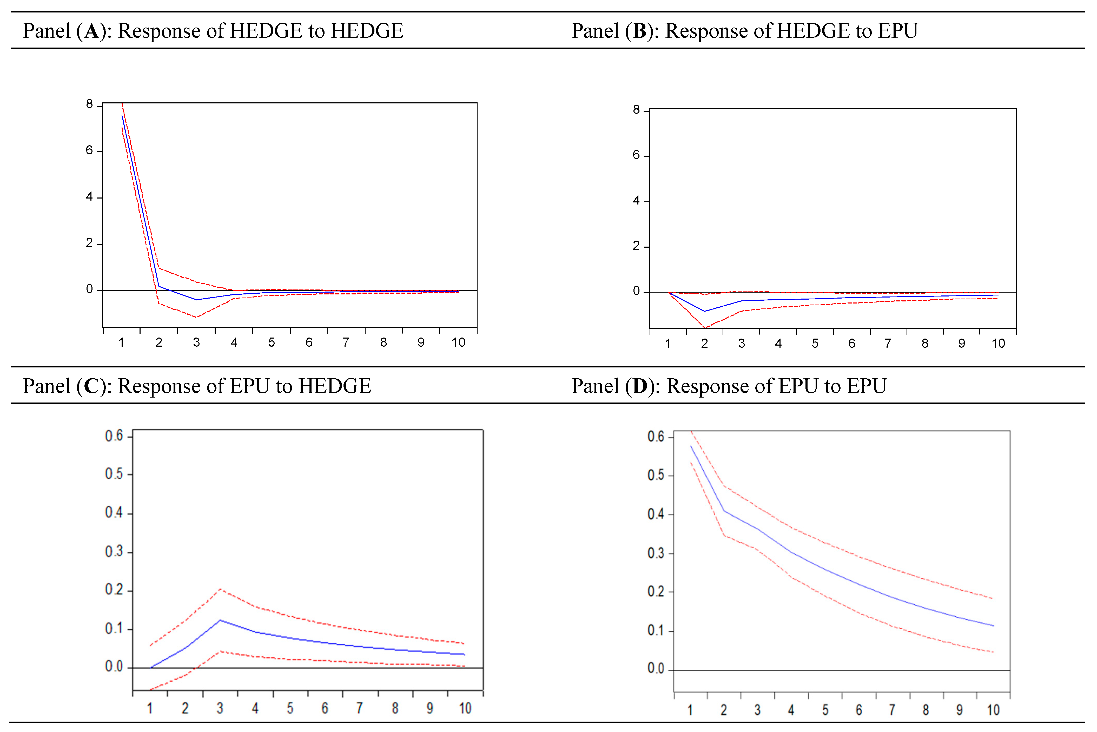
5.7.4. Impulse Response

The impulse response function studies how the variables respond when some external shock hits the system. Table 12 examines the response of EPU (hedge) on EPU (hedge) and hedge (EPU). Panel (A) shows that the response of EPU on EPU is positive but decreases up to period four and increases until period seven before falling afterward. EPU makes a U-shaped curve for 10 periods, and the reverse is valid for the response of EPU on the hedge, which makes an inverse U-shaped curve. In Panel (B) of Table 12, the response of hedge on EPU and hedge is put under a scanner, which follows a wave pattern. As shown in the table, the values change from positive to negative from the first to the third period, become positive until the fifth lag, and decrease afterward. The response of the hedge on the hedge also follows a similar pattern. Figure 2 complements our findings reported in Table 12.

6. Conclusions

We begin this article with the penultimate aim to shed light on the implication of policy uncertainty on the momentum anomaly. Our results demonstrate the negative association between the news-based measure developed by Baker, Bloom, and Davis and a momentum hedge portfolio. EPU is also negatively related to WML, which corroborates our findings for the hedge portfolio. Second, variability in momentum profits is linked to the business cycle. Third, alpha coefficients are significant for short and hedge portfolio during the period of high EPU but insignificant during the low EPU period. Fourth, EPU is positively associated with short portfolio return to the tune of 1.037 percent excess returns. The hedge portfolio is negatively related to EPU. Nevertheless, EPU becomes insignificant in the presence of four factors. Further, we demonstrate that half of the macroeconomic variables, along with EPU, turns out to be statistically significant. Fifth, hedge portfolio returns are influencing EPU but not the other way around in the short run. Last, the hedge portfolio is found to have a significant relationship with EPU.
The findings of this article contribute to the existing strand of literature on the growing nexus between EPU and the hedge portfolio. Our findings complement the findings of Gu et al. (2021) and Xavier and Vasconcelos (2019) and cement the prominence of EPU in exploring the stock return momentum. We use an umbrella of macroeconomic variables to substantiate the relation between EPU and momentum. Our findings open avenues for momentum and contrarian investors. This warrants the attention of style investors to consider the prevailing state of policy uncertainty while formulating and executing their trading strategy.
As with any study of a scientific nature, our work also has limitations, which may be reduced in future analysis. In fact, although the literature on the subject is very vast (Al-Thaqeb and Algharabali 2019), there are still gaps in knowledge about the importance of uncertainty in economic policy. Our article intends to cover some of those gaps, but it could be extended, for example, in the construction of a theoretical model based on others of a seminal nature in economic policy, where the relations between the influence of society are established and vice versa.
Results have shown that EPU is a crucial determinant to explain cross-sectional and time-series variation in momentum profits in the short run and long run. This requires the further interest of academics to explore the existence of a momentum anomaly by using EPU as a significant factor. There is a possibility that the EPU of different countries might behave differently for momentum profits. We leave this as a direction for future research.

Author Contributions

All the authors have contributed equally. All authors have read and agreed to the published version of the manuscript.

Funding

This research received no external funding.

Data Availability Statement

Data sharing not applicable.

Conflicts of Interest

The authors declare no conflict of interest.

References

  1. Addoum, Jawad M., Stefanos Delikouras, Da Ke, and Alok Kumar. 2019. Underreaction to political information and price momentum. Financial Management 48: 773–804. [Google Scholar] [CrossRef]
  2. Adjei, Frederick A., and Mavis Adjei. 2017. Economic policy uncertainty, market returns and expected return predictability. Journal of Financial Economic Policy 9: 242–59. [Google Scholar] [CrossRef]
  3. Al-Thaqeb, Saud Asaad, and Barrak Ghanim Algharabali. 2019. Economic policy uncertainty: A literature review. The Journal of Economic Asymmetries 20: e00133. [Google Scholar] [CrossRef]
  4. Antonakakis, Nikolaos, Ioannis Chatziantoniou, and George Filis. 2014. Dynamic spillovers of oil price shocks and economic policy uncertainty. Energy Economics 44: 433–47. [Google Scholar] [CrossRef] [Green Version]
  5. Antoniou, Antonios, Herbert Y. T. Lam, and Krishna Paudyal. 2007. Profitability of momentum strategies in international markets: The role of business cycle variables and behavioural biases. Journal of Banking & Finance 31: 955–72. [Google Scholar]
  6. Antoniou, Constantinos, John A. Doukas, and Avanidhar Subrahmanyam. 2013. Cognitive dissonance, sentiment, and momentum. Journal of Financial and Quantitative Analysis 48: 245–75. [Google Scholar] [CrossRef] [Green Version]
  7. Aretz, Kevin, Söhnke M. Bartram, and Peter F. Pope. 2010. Macroeconomic risks and characteristic-based factor models. Journal of Banking and Finance 34: 1383–99. [Google Scholar] [CrossRef] [Green Version]
  8. Avramov, Doron, and Tarun Chordia. 2006. Asset pricing models and financial market anomalies. The Review of Financial Studies 19: 1001–40. [Google Scholar] [CrossRef]
  9. Avramov, Doron, Si Cheng, and Allaudeen Hameed. 2016. Time-varying liquidity and momentum profits. Journal of Financial and Quantitative Analysis 51: 1897–923. [Google Scholar]
  10. Bahmani-Oskooee, Mohsen, and Majid Maki-Nayeri. 2019. Asymmetric effects of policy uncertainty on the demand for money in the United States. Journal of Risk and Financial Management 12: 1. [Google Scholar] [CrossRef] [Green Version]
  11. Baker, Scott R., Nicholas Bloom, Brandice Canes-Wrone, Steven J. Davis, and Jonathan Rodden. 2014. Why has US policy uncertainty risen since 1960? American Economic Review 104: 56–60. [Google Scholar] [CrossRef] [Green Version]
  12. Baker, Scott R., Nicholas Bloom, and Steven J. Davis. 2016. Measuring economic policy uncertainty. The Quarterly Journal of Economics 131: 1593–636. [Google Scholar] [CrossRef]
  13. Bernal, Oscar, Jean-Yves Gnabo, and Grégory Guilmin. 2016. Economic policy uncertainty and risk spillovers in the Eurozone. Journal of International Money and Finance 65: 24–45. [Google Scholar] [CrossRef]
  14. Brogaard, Jonathan, and Andrew Detzel. 2015. The asset-pricing implications of government economic policy uncertainty. Management Science 61: 3–18. [Google Scholar] [CrossRef] [Green Version]
  15. Carhart, Mark. M. 1997. On persistence in mutual fund performance. The Journal of Finance 52: 57–82. [Google Scholar] [CrossRef]
  16. Chan, Louis K. C., Narasimhan Jegadeesh, and Josef Lakonishok. 1999. The profitability of momentum strategies. Financial Analysts Journal 55: 80–90. [Google Scholar] [CrossRef]
  17. Chordia, Tarun, and Lakshmanan Shivakumar. 2002. Momentum, business cycle, and time-varying expected returns. The Journal of Finance 57: 985–1019. [Google Scholar] [CrossRef]
  18. Cooper, Michael J., Roberto C. Gutierrez Jr., and Allaudeen Hameed. 2004. Market states and momentum. The Journal of Finance 59: 1345–65. [Google Scholar] [CrossRef] [Green Version]
  19. Du, Ding, Zhaodan Huang, and Bih-Shuang Liao. 2009. Why is there no momentum in the Taiwan stock market? Journal of Economics and Business 61: 140–52. [Google Scholar] [CrossRef]
  20. Fama, Eugene F., and Kenneth R. Frence. 2012. Size, value, and momentum in international stock returns. Journal of Financial Economics 105: 457–72. [Google Scholar] [CrossRef]
  21. Friedman, Milton. 1953. Effects of Full Employment Policy on Economic Stability: A Formal Analysis. In Essays in Positive Economics. Chicago: University of Chicago Press, pp. 117–32. [Google Scholar]
  22. Galariotis, Emilios, and Konstantinos Karagiannis. 2020. Cultural dimensions, economic policy uncertainty, and momentum investing: International evidence. The European Journal of Finance, 1–18. [Google Scholar] [CrossRef]
  23. Griffin, John M., Xiuqing Ji, and J. Spencer Martin. 2003. Momentum investing and business cycle risk: Evidence from pole to pole. The Journal of Finance 58: 2515–47. [Google Scholar] [CrossRef]
  24. Gu, Ming, Minxing Sun, Yangru Wu, and Weike Xu. 2021. Economic policy uncertainty and momentum. Financial Management, 1–23. [Google Scholar] [CrossRef]
  25. Jegadeesh, Narasimhan, and Sheridan Titman. 1993. Returns to buying winners and selling losers: Implications for stock market efficiency. The Journal of Finance 48: 65–91. [Google Scholar] [CrossRef]
  26. Jegadeesh, Narasimhan, and Sheridan Titman. 2001. Profitability of momentum strategies: An evaluation of alternative explanations. The Journal of Finance 56: 699–720. [Google Scholar] [CrossRef] [Green Version]
  27. Jegadeesh, Narasimhan, and Sheridan Titman. 2011. Momentum. Annual Review of Financial Economics 3: 493–509. [Google Scholar] [CrossRef]
  28. Kelly, Bryan, Ľuboš Pástor, and Pietro Veronesi. 2016. The price of political uncertainty: Theory and evidence from the option market. The Journal of Finance 71: 2417–80. [Google Scholar] [CrossRef]
  29. Korajczyk, Robert A., and Ronnie Sadka. 2004. Are momentum profits robust to trading costs? The Journal of Finance 59: 1039–82. [Google Scholar] [CrossRef]
  30. Kumar, Ameet, Muhammad Ramzan Kalhoro, Rakesh Kumar, Niaz Hussain Ghumro, Sarfraz Ahmed Dakhan, and Vikesh Kumar. 2020. Decomposing the Effect of Domestic and Foreign Economic Policy Uncertainty Shocks on Real and Financial Sectors: Evidence from BRIC Countries. Journal of Risk and Financial Management 13: 315. [Google Scholar] [CrossRef]
  31. Kydland, Finn E., and Edward C. Prescott. 1977. Rules rather than discretion: The inconsistency of optimal plans. Journal of Political Economy 85: 473–91. [Google Scholar] [CrossRef] [Green Version]
  32. Lesmond, David A., Michael J. Schill, and Chunsheng Zhou. 2004. The illusory nature of momentum profits. Journal of Financial Economics 71: 349–80. [Google Scholar] [CrossRef]
  33. Liow, Kim Hiang, Wen-Chi Liao, and Yuting Huang. 2018. Dynamics of international spill overs and interaction: Evidence from financial market stress and economic policy uncertainty. Economic Modelling 68: 96–116. [Google Scholar] [CrossRef]
  34. Liu, Laura Xiaolei, and Lu Zhang. 2008. Momentum profits, factor pricing, and macroeconomic risk. The Review of Financial Studies 21: 2417–48. [Google Scholar] [CrossRef]
  35. Pástor, Ľuboš, and Pietro Veronesi. 2013. Political uncertainty and risk premia. Journal of Financial Economics 110: 520–45. [Google Scholar] [CrossRef] [Green Version]
  36. Phan, Dinh Hoang Bach, Susan Sunila Sharma, and Vuong Thao Tran. 2018. Can economic policy uncertainty predict stock returns? Global evidence. Journal of International Financial Markets, Institutions and Money 55: 134–50. [Google Scholar] [CrossRef]
  37. Rouwenhorst, K. Geert. 1999. Local return factors and turnover in emerging stock markets. The Journal of Finance 54: 1439–64. [Google Scholar] [CrossRef]
  38. Swinkels, Laurens. 2004. Momentum investing: A survey. Journal of Asset Management 5: 120–43. [Google Scholar] [CrossRef]
  39. Tsai, I-Chun. 2017. The source of global stock market risk: A viewpoint of economic policy uncertainty. Economic Modelling 60: 122–31. [Google Scholar] [CrossRef]
  40. Van der Ploeg, Frederick. 1989. The political economy of overvaluation. Economic Journal 99: 850–55. [Google Scholar] [CrossRef]
  41. Xavier, Gustavo, and Lucas N. C. Vasconcelos. 2019. The Impact of Foreign and Country-Specific Economic Policy Uncertainty on the Local Momentum Effect. Available online: https://papers.ssrn.com/sol3/papers.cfm?abstract_id=3187600 (accessed on 1 December 2020).
  42. Zaremba, Adam. 2019. The cross section of country equity returns: A review of empirical literature. Journal of Risk and Financial Management 12: 165. [Google Scholar] [CrossRef] [Green Version]
1
The first component comprises search results gathered from 10 leading newspapers daily in the United States, where newspaper articles deliberating over economic policy are incorporated. An article is associated with economic uncertainty when words such as ‘uncertain,’ ‘economic,’ ‘legislation,’ and ‘federal reserve’ have be used at least once in the newspaper article. The second component is created by the inclusion of “tax code provisions” that are slated to elapse over the coming 10 years. The last component collects data from “Federal Reserve Bank of Philadelphia’s Survey of Professional Forecasters” to compute the level of dispersion among individual forecasters relating to macroeconomic policy variables. The weights assigned to the first, second, and third components are 0.5, 0.17, and 0.33, respectively.
2
For example, Jegadeesh and Titman (2001) using a sample of NASDAQ, NYSE, and AMEX listed stocks from 1990–1998, documented that past winners outperform past losers by approximately 1.39% per month. This is consistent with the results reported in Jegadeesh and Titman (1993), i.e., 1.31% per month. Later, Rouwenhorst (1999) using a sample of 20 emerging markets, found that the average return from the long-short momentum strategy is 0.39% per month. Griffin et al. (2003) reported that the average monthly momentum profit from a winner-minus-loser strategy is 0.59%, 0.77%, 1.63%, and 0.32% for the U.S, Europe, Africa, and Asia, respectively. It is worthwhile to note that the higher returns observed by Jegadeesh and Titman (1993, 2001), Rouwenhorst (1999), and Griffin et al. (2003) do not necessarily imply investor profits due to higher transactions costs (Swinkels 2004; Lesmond et al. 2004). Korajczyk and Sadka (2004) found that when price impact is ignored and transaction costs are proportional costs equal to the effective and quoted spreads, the momentum strategy earns significant profits. Similarly, Lesmond et al. (2004) failed to reject profitability in all momentum strategies, even after considering transaction cost aspects.
3
See www.policyuncertainty.com/index.html, accessed on 20 December 2020.
4
5
See fred.stlouisfed.org/, accessed on 24 December 2020.
6
See www.nber.org/cycles/cyclesmain.html, accessed on 22 December 2020.
7
M3 is utilized by the central bank to direct monetary policy to control inflation. This implies that M3 has an indirect impact on inflation via monetary policy. We examined the multicollinearity among macroeconomic variables in Table 9. VIF for the regression model in Table 9 turned out to be 1.24, 1.19, and 1.16 for inflation and money supply, respectively. To further clear our suspicion towards the relationship between inflation and money supply, we checked the correlation between the two variables, which turned out to −0.1261.
Figure 1. (a) Co-movement between EPU and momentum portfolios. (b) Co-movement between EPU and WML (hedge portfolio).
Jrfm 14 00141 g001
Figure 2. Impulse response function graphs. The figure displays the impulse response of EPU (hedge) on EPU (hedge) and hedge (EPU) across the four panels. Cholesky Ordering is utilized to obtain the results.
Jrfm 14 00141 g002
Table 1. Descriptive statistics.
VariableObs.MeanStd. Dev.MinMax
HEDGE4071.1027.623−45.5826.15
MKTRF4070.6634.361−23.2412.47
SMB4070.0433.078−16.8721.71
HML4070.1922.867−11.1012.90
WML4070.5624.496−34.3918.36
EPU407108.11731.3457.203245.127
Notes: The table reports the descriptive statistics for the hedge portfolio (HEDGE), market risk premium (MKTRF), small minus big size factor (SMB), the high minus low book to market factor (HML), winner minus loser factor (WML), and economic policy uncertainty (EPU).
Table 2. Pairwise correlation.
Variables(1)(2)(3)(4)(5)(6)
(1) HEDGE1.000
(2) MKTRF−0.208 *1.000
(3) SMB0.0030.210 *1.000
(4) HML−0.190 *−0.217 *−0.266 *1.000
(5) WML0.919 *−0.171 *0.048−0.199 *1.000
(6) EPU−0.115 *0.0750.073−0.103 *−0.140 *1.000
Notes: The table reports the pairwise correlation among the hedge portfolio (HEDGE), market risk premium (MKTRF), small minus big size factor (SMB), the high minus low book to market factor (HML), winner minus loser factor (WML), and economic policy uncertainty (EPU). * shows significance at the 5 percent level.
Table 3. Business cycle and momentum.
Expansionary PeriodContractionary Period
December1982–July 19900.0149 (3.84)August 1990–March 1991−0.0172 (−0.54)
April 1991–March 20010.0034 (0.53)April 2001–November 2001−0.0216 (−0.52)
December 2001–December 20070.0032 (0.73)January 2008–June 2009−0.0432 (−1.27)
Notes: The table presents the hedge portfolio returns (HEDGE) during two phases of the business cycle—expansionary and contractionary period as per definition by NBER. T-statistics are reported in parenthesis.
Table 4. Four factors alpha and momentum portfolio.
(1)
Long
(2)
Short
(3)
Hedge
MKTRF1.176 *** (0.0364)1.269 *** (0.0457)−0.092 * (0.0509)
SMB0.355 *** (0.0421)0.450 *** (0.0492)−0.095 * (0.0530)
HML−0.121 ** (0.0521)−0.035 (0.0847)−0.086 (0.0824)
WML0.498 *** (0.0317)−1.036 *** (0.0476)1.534 *** (0.0582)
CONS0.031 (0.108)−0.290 * (0.157)0.322 * (0.167)
N407407407
Adj. R20.8980.8800.847
F276.4305.8175.3
Notes: The table presents the time-series regression results for long, short, and hedge portfolios across three models from Equation (1), respectively. Four factors, namely, market risk premium (MKTRF), small minus big size factor (SMB), high minus low book to market factor (HML), and winner minus loser factor (WML), were employed. Standard errors are reported in parentheses. *, **, and *** denote the significance at 10%, 5%, and 1% percent.
Table 5. GRS test.
Table 5. GRS test.
Mean Alphat-Statp ValueMean Adj. R2Mean SEMean |a|SR
J00.3224.480.0340.84690.15270.32180
J10.3214.420.0350.84690.15270.32180.1084
Notes: The table reports the results of the GRS test. Mean alpha denotes the average standard error of the intercepts, and SR represents the Sharpe ratio for the intercepts. The critical values of the GRS statistic for all models are: 90%: 1.41; 95%: 1.56; 97.5%: 1.69; 99%: 1.86; and 99.9%: 2.25.
Table 6. High EPU and the four factor asset pricing model.
(1)(2)(3)
LongShortHedge
MKTRF1.176 *** (0.0345)1.248 *** (0.0580)−0.0723 (0.0616)
SMB0.494 *** (0.0541)0.343 *** (0.0973)0.151 (0.0968)
HML−0.0287 (0.0467)0.222 ** (0.110)−0.251 ** (0.118)
WML0.497 *** (0.0298)−1.104 *** (0.0767)1.601 *** (0.0892)
CONS0.0391 (0.134)−0.458 * (0.240)0.497 ** (0.246)
N204204204
Adj. R20.9100.8950.867
F365.9232.487.74
Notes: The table presents the time-series regression results for long, short, and hedge portfolios across three models from Equation (2) for a high EPU period, respectively. Four factors, namely, market risk premium (MKTRF), small minus big size factor (SMB), high minus low book to market factor (HML), and winner minus loser factor (WML), were employed. Standard errors are reported in parentheses. *, **, and *** denote the significance at 10%, 5%, and 1% percent.
Table 7. Low EPU and four factor asset pricing model.
(1)
Long
(2)
Short
(3)
Hedge
MKTRF1.133 *** (0.0637)1.222 *** (0.0551)−0.0892 (0.0769)
SMB0.239 *** (0.0598)0.399 *** (0.0615)−0.160 ** (0.0693)
HML−0.286 *** (0.106)−0.373 *** (0.112)0.0872 (0.123)
WML0.518 *** (0.0601)−1.057 *** (0.0547)1.575 *** (0.0665)
CONS−0.0176 (0.157)0.0535 (0.173)−0.0710 (0.194)
N203203203
Adj. R20.8960.8700.826
F114.3223.0159.9
Notes: The table presents the time-series regression results for long, short, and hedge portfolios across three models from Equation (2) for a low EPU period, respectively. Four factors, namely, market risk premium (MKTRF), small minus big size factor (SMB), high minus low book to market factor (HML) and winner minus loser factor (WML), are employed. Standard errors are reported in parentheses. **, and *** denote the significance at 5%, and 1%, respectively.
Table 8. Time series regression and EPU.
(1)(2)(3)(4)(5)(6)
LongLongShortShortHedgeHedge
EPU0.160 (0.354)−0.0314 (0.103)1.037 + (0.599)−0.150 (0.180)−0.878 + (0.464)0.119 (0.186)
MKTRF 1.176 *** (0.0364) 1.269 *** (0.0458) −0.0928 + (0.0511)
SMB 0.355 *** (0.0421) 0.453 *** (0.0488) −0.0972 + (0.0527)
HML −0.122 * (0.0516) −0.0413 (0.0863) −0.0809 (0.0835)
WML 0.497 *** (0.0321) −1.042 *** (0.0455) 1.539 *** (0.0563)
CONS1.083 *** (0.299)0.0322 (0.108)−0.0194 (0.426)−0.286 + (0.156)1.102 ** (0.376)0.319 + (0.165)
N407407407407407407
adj. R2−0.0020.8970.0120.8800.0110.847
F0.203221.33.003270.23.572159.9
Notes: The table presents the time-series regression results for long, short, and hedge momentum portfolios across different model specification from Equations (3) and (4), respectively. Four factors, namely, market risk premium (MKTRF), small minus big size factor (SMB), high minus low book to market factor (HML), and winner minus loser factor (WML), were employed. Standard errors are reported in parentheses. +, *, **, and *** denote the significance at 10%, 5%, 1%, and 0.1%.
Table 9. Macroeconomic factors and EPU.
Hedge
DIV11.43 (8.033)
INFLATION1.436 * (0.812)
M3−55.07 (287.9)
YIELD−2.970 (2.313)
DEFAULT−15.56 ** (7.059)
TERM−4.938 ** (2.136)
IIP0.461 (0.713)
EPU0.0299 * (0.0171)
CONS0.600 (0.711)
N406
Adj. R20.091
F3.662
Notes: The table reports the regression results for EPU and macroeconomic variables, which includes dividend yield (DIV), consumer price index (INFLATION), money supply (M3), the yield on 3-month treasury bills (YIELD), default spread (DEFAULT), term spread (TERM), and the index of industrial production (IIP). Standard errors are reported in parentheses. *, and ** denote the significance at 10%, and 5%.
Table 10. Vector autoregression results.
Coef.Std. Err.p > z95% Conf.Interval
Panel (A): EPU as the dependent variable
EPU
L1.0.7260.0620.0000.6040.848
L2.−0.0930.0780.233−0.2450.060
L3.0.0050.0780.953−0.1490.158
L4.0.2730.0700.0000.1370.410
HEDGE
L1.0.1550.1590.328−0.1560.467
L2.0.4210.1580.0080.1120.730
L3.−0.0900.1520.555−0.3880.208
L4.0.3260.1400.0200.0510.600
Constant9.4774.5740.0380.51318.441
Panel (B): HEDGE as the dependent variable
EPU
L1.−0.0180.0220.411−0.0600.025
L2.−0.0070.0270.807−0.0600.046
L3.0.0160.0270.548−0.0370.070
L4.−0.0130.0240.581−0.0610.034
HEDGE
L1.0.0880.0550.112−0.0210.196
L2.−0.0190.0550.725−0.1270.088
L3.0.0130.0530.813−0.0910.116
L4.0.1610.0490.0010.0660.257
Constant3.8371.5920.0160.7176.956
Notes: The table exhibits the VAR results between EPU and HEDGE portfolio returns up to four lags in two panels.
Table 11. Vector error correction model.
Cointegrating equation:Cointegrating Equation (1)
EPU (−1)1.000000
HEDGE (−1)51.09338 ***
(5.35805)
C−162.5485
Error Correction:D(EPU)D(HEDGE)
Cointegrating Equation (1)0.018317 ***−0.018495 ***
(0.00508)(0.00215)
D (EPU (−1))−0.328359 ***−0.009266
(0.05121)(0.02168)
D (EPU (−2))−0.306039 ***−0.014115
(0.05164)(0.02186)
D (EPU (−3))−0.271631 ***0.036195
(0.05208)(0.02205)
D (EPU (−4))−0.128718 ***0.054237 ***
(0.05032)(0.02130)
D (HEDGE (−1))−0.753648 ***−0.031366
(0.23890)(0.10113)
D (HEDGE (−2))−0.374986 *−0.056872
(0.20939)(0.08864)
D (HEDGE (−3))−0.386537 **−0.011666
(0.16870)(0.07142)
D (HEDGE (−4))−0.0935850.066331
(0.12028)(0.05092)
C−0.035858−0.008797
(0.88857)(0.37616)
Adj. R20.1521580.499365
F8.97625145.33162
Notes: The table reports the vector error correction model results for EPU and HEDGE portfolios up to four lags. Standard errors are reported in parentheses. *, **, and *** denote the significance at 10%, 5%, and 1%.
Table 12. Impulse response function results.
Panel (A): Response of EPUPanel (B): Response of HEDGE
PeriodEPUHEDGEPeriodEPUHEDGE
117.792620.00000010.1872227.529812
212.310281.3721272−0.4894990.178284
38.8723943.8304543−0.444385−0.225921
46.7400642.61284140.5995740.217503
57.8162504.09335450.7282190.584200
610.137124.1587926−0.614950−0.396321
710.233873.8716797−0.496040−0.053057
89.4638143.6475088−0.186526−0.015110
99.1461903.8406839−0.0294230.035556
109.1464033.92571310−0.140596−0.147335
Notes: The table presents the impulse response of EPU (hedge) on EPU (hedge) and hedge (EPU) in Panel (A) and (B), respectively. Cholesky ordering was utilized to obtain the results.
Publisher’s Note: MDPI stays neutral with regard to jurisdictional claims in published maps and institutional affiliations.

