Creating Unbiased Machine Learning Models by Design

Abstract

Unintended bias against protected groups has become a key obstacle to the widespread adoption of machine learning methods. This work presents a modeling procedure that carefully builds models around protected class information in order to make sure that the final machine learning model is independent of protected class status, even in a nonlinear sense. This procedure works for any machine learning method. The procedure was tested on subprime credit card data combined with demographic data by zip code from the US Census. The census data serves as an imperfect proxy for borrower demographics but serves to illustrate the procedure.

1. Introduction

The greatest challenge to the widespread adoption of machine learning methods in credit underwriting is the risk of violating the Fair Credit Reporting Act (FCRA) (2012) by providing recommendations that are adversely correlated with protected class status such as race, gender, religion, zipcode, etc. The challenge arises from the ability of machine learning methods to leverage superficially unrelated data to infer structure that is highly correlated with protected class status, even though the input data did not explicitly include any such factors. Past FCRA rulings indicate that a model’s forecasts cannot be adjusted after development to remove bias. Rather, the model must be developed initially to lack any prohibited correlations.

Our work creates a two-step modeling process to prevent the final model from having any structures, linear correlation, or nonlinear dependence related to protected class status. This is accomplished by first creating a model that predicts loan output using only prohibited information. This is used as a fixed input to a second model that only uses seemingly appropriate information but that could otherwise exhibit correlations to protected class status. When the model is used for loan underwriting, the first model on restricted information is replaced with a single average loss rate, which serves as what would have been the intercept term of the model using appropriate inputs.

This seemingly simple procedure has some subtle consequences and benefits and is ideally suited to unconstrained or uncontrollable machine learning models. Other groups have developed bias measurement toolkits intended to help researchers measure potential bias and adjust their models appropriately (Bellamy et al. 2019; Saleiro et al. 2018). Our goal is to develop a modeling procedure that cannot be biased as a consequence of its construction, guaranteeing that it would pass such tests.

The article begins with a discussion of bias in machine learning and unique challenges in lending. Section 3 describes the test data, including census data and performance of subprime credit cards. Section 4 describes the modeling methods used for this test. Section 5 and Section 6 provide the model estimation details and test results.

2. Definitions of Bias

Concerns about bias in machine learning are widespread. Examples of failures in the criminal justice system (Završnik 2019), hiring at Amazon (Dastin 2018), suggestions of problems with the Apple Card (Knight 2019), and facial recognition (Herlitz and Lovén 2013) are just a few (O’neil 2016). Notably, the defense of Apple Card against gender bias in the assignment of credit lines was that none of the inputs included gender. However, gender blindness does not guarantee gender neutrality, which is the essence of the problem in applying machine learning to credit risk modeling.

Mehrabi et al. (2021) put all the potential sources of bias into two broad categories: bias in the data or bias in the algorithm. Within these they define 23 kinds of bias. Among the problems that can occur in machine learning, overfitting is the most pervasive and probably the most studied (Gençay and Qi 2001). Furthermore, neural networks can be susceptible to a “recency” bias, wherein the model’s parameters are more heavily tuned to the most recent training data (Gradojevic et al. 2009). Furthermore, data snooping bias (Sermpinis et al. 2016) occurs when models are trained multiple times on the same data set, eventually making the test data part of the training data or simply causing researchers to misjudge the significance of their results.

However, the bias problem in lending is actually different from all 23 identified by Mahrabi. Our data may faithfully represent what is in society and have no knowledge of protected class status, and yet correlate to such status in violation of FCRA. This is an unintended ethical bias (Shadowen 2019). So how do we remove an ethical bias with no knowledge of the ethical conflict? The truth is that we cannot. Judging a model on ethical bias after it was created without knowledge of protected class status is a doomed approach, and yet is how regulators appear to be approaching the problem. To prevent ethical bias, we must know that we are biased or at least where we have risk of bias. Having color-blind data does not protect us from creating models that are color-biased.

With linear methods, we generally feel safe in saying that no information on protected class status was given to the model, so the results are unbiased. The same cannot be said of machine learning (Feldman et al. 2015; Prince and Schwarcz 2019), especially when given alternate inputs. Big data and sophisticated modeling approaches create significant risks of unfair treatment (O’neil 2016). Unfortunately, a linear mindset underlies US regulations.

One such example showed that the digital footprint of an online borrower was as predictive as FICO score, yet all of those digital footprint data elements probably correlate to protected class status (Berg et al. 2018). Excluding protected data is insufficient to assert that the final model’s forecasts do not correlate to protected status. Simple linear correlation is the standard for finding discrimination.

We refer to this as an unintended bias, because the model developer may take no actions specifically intended to create such bias and may themselves be unaware of the presence of bias. The unawareness of bias can easily occur, because except for mortgage reporting requirements, lenders are actually prohibited from collecting data on protected class status in a way that would allow a credit risk model developer to conclusively test the models. The best that can be done today is to guess ethnicity from last names, as regulators have been attempting, and yet that process is prone to being unfair as well.

The task then becomes creating a model that is ethically unbiased, even though the data set provides no information against which to test for bias. To be blunt, that is practically impossible for the most well-meaning human agent. For an automated algorithm, failure is assured, eventually. The solutions will be legal as much as statistical (Lehr and Ohm 2017).

For the present research, we imagine a world where protected class status is included in the data set, so that we can intentionally prevent bias and test for success. This is often true in applications outside lending, such as Amazon’s hiring data or criminal justice data, on which we hope this approach might be tested. In order to test the approach on lending data, we will use US Census data by 5-digit zip code as a proxy for who the borrowers might have been.

3. Data

Data were obtained from a Near Prime to Subprime credit card portfolio, defined as less than 700 FICO. The data sample contained 146,500 accounts originated between 2005 and 2019, which were split half for testing and half for training. Averaged across the observed period from 2007 through 2019, the default rate was 6.2%. We specifically avoided data from the SARS-CoV-2 (COVID-19) pandemic. Performance data during this period was strongly affected by job losses but also government support programs and lender forbearance programs that are not well-captured in the data. In addition, these programs are not yet closed at the time of this research, so the ultimate default outcomes are not yet known (Breeden et al. 2021).

The later analysis will create models using only that information available at origination to predict later defaults. The portfolio data included the following metrics:

• Original score
• Original interest rate
• Subcategory
• Credit limit
• Balance transfer
• Total loan balance
• Total deposits
• 5-digit Zipcode

Total loan balance and total deposits refer to the complete relationship of the borrower with the lender across all products.

The US Census data was obtained from the 2010 census, which had the best overlap to the available loan data. The following fields were extracted, specifically because they would not be FCRA compliant.

• Median age
• Male to female ratio
• Persons per household
• Asian fraction
• Black fraction
• Native American fraction
• Native Hawaiian fraction
• Hispanic fraction

The origination data from the loan portfolio was matched by 5-digit zipcode to incorporate the census data. We cannot know the actual age, gender, or ethnicity of the borrower, but simply assigned the probability or average of these values from the census data for the area where they reside.

Table 1. Correlation coefficients were computed between census measures and loan data in the corresponding zipcodes. 95% confidence intervals are shown.

	Bureau Score	Interest Rate	Credit Limit
Median Age	0.0435 (0.0418, 0.0451)	$-0.0573(-0.0596,-0.0551)$	0.0691  (0.0675, 0.0708)
Male-Female Ratio	$-0.0068(-0.0084,-0.0051)$	$0.0007(-0.0016,0.0029)$	$-0.0096(-0.0112,-0.0079)$
Persons per Household	$-0.0033(-0.0050,-0.0017)$	0.0675 (0.0653, 0.0697)	$-0.0417(-0.0433,-0.0401)$
Asian Fraction	$-0.0012(-0.0029,0.00045)$	0.0279 (0.0256, 0.0301)	0.0020 (0.00042, 0.0037)
Black Fraction	$-0.0117(-0.0133,-0.0100)$	0.0518 (0.0495, 0.0540)	$-0.0476(-0.0492,-0.0459)$
Native American Fraction	$-0.0034(-0.0050,-0.0017)$	$0.0011(-0.0012,0.0033)$	$-0.0145(-0.0161,-0.0129)$
Native Hawaiian Fraction	$-0.0059(-0.0076,-0.0042)$	0.0116 (0.0094, 0.0139)	$-0.0107(-0.0123,-0.0091)$
Hispanic Fraction	$-0.0074(-0.0091,-0.0057)$	0.0806 (0.0783, 0.0828)	$-0.0387(-0.0403,-0.0371)$

shows the correlations between the assigned census values and the loan data. In almost all cases, statistically significant correlations are found, even though those correlations are slight. Correlations to interest rate and credit limit are excusable when the same data correlates to the original credit bureau score used for underwriting.

This table is not evidence of bias. At most, it is evidence of a cultural problem that non-white ethnic groups in the US are poorer than corresponding white borrowers. Notably, in almost every case, when the percentage of an ethnic group rises and bureau scores decline, interest rates rise and credit limits decline. The movement of interest rates and credit limits relative to bureau scores is financially reasonable. The correlation between ethnicity and bureau score is where the cultural problem lies.

The challenge faced by lenders is proving a lack of bias. The portfolio analyzed here used underwriting methods that passed regulatory review on the basis that they did not have any protected class status inputs; the models were linear, and the sensitive factors in the model were to the borrowers’ past financial performance, as measured at the credit bureaus. In a world of alternate data and machine learning, even when everything is undertaken properly, residual correlations to protected class are almost certain unless explicit preventative measures can be taken.

4. Model Development

A significant amount of research is being conducted on how to identify and mitigate disparate impacts from machine learning. Current methods can largely be grouped into two approaches. The first is to modify the input data to prevent models from finding biases (Feldman et al. 2015; Kamiran and Calders 2010; Zemel et al. 2013; Zliobaite et al. 2011). The second approach modifies the learning algorithm to add constraints that would enforce fairness conditions (Fish et al. 2015; Kamishima et al. 2012; Kozodoi et al. 2021; Luo et al. 2015; Zafar et al. 2015).

Among the research into how to modify the input data, Feldman et al. (2015) identify the specific input factors causing the problem and adjust them the least amount possible so as to prevent an assessment of bias. Kamiran and Calders (2010) create a preferential sampling of the input data to eliminate the risk of creating biased models. Zliobaite et al. (2011) seek to modify the dependent variable in the input training data to remove historic bias prior to model training. Zemel et al. (2013) formulate fairness as a problem of finding an optimal representation of the data file, simultaneously obfuscating information about protected class status.

For research into how to modify the model training or use, Luo et al. (2015) create a discrimination-aware association rule classifier incorporating a discrimination adjustment during classifier training. Fish et al. (2015) modified the hypothesis output of the AdaBoost classification algorithm by shifting the decision boundary for the protected class. Kozodoi et al. (2021) review methods in credit scoring for incorporating fairness criteria into the machine learning development process. Kamishima et al. (2012) create a regularization approach applicable to any model that removes prediction bias. Zafar et al. (2015) explain a mechanism to design fair classifiers via tunable decision boundaries to apply varying degrees of fairness.

Correlation is a simple linear measure. A simple, even-ordered polynomial relationship between the default outcome and a restricted input could discriminate against borrowers and yet slip past a linear correlation test. To comply with the spirit of the law and the ethics behind the law, our approach seeks to make sure that nonlinear methods such as the many machine learning approaches do not find pockets of predictability relative to restricted inputs.

To achieve nonlinear independence between credit risk modeling and restricted inputs, we propose the following analysis steps:

• Perform age–period–cohort analysis to quantify lifecycle and environment.
• Create a scoring model via regression or machine learning using only restricted inputs and APC functions as a fixed offset.
• Create a second scoring model via regression or machine learning using only apparently acceptable inputs with the restricted scoring model and APC functions as a fixed offset.
• Create the forecasts from the second scoring model with the restricted scoring model inputs set to zero.

The first step, using age–period–cohort analysis, allows us to normalize the default performance for changing macroeconomic environments, seasonality, and the lifecycle versus age of the account. This is optional as part of creating a score, but it serves both to stabilize the score estimation through different phases of the economic environment and to allow the model to predict calibrated probability of default using macroeconomic scenarios (Breeden and Thomas 2008).

The second step of building an APC Score using only restricted inputs and with the APC lifecycle and environment as fixed inputs is designed to provide a worst-case model. What is the most structure that can be explained statistically due to restricted inputs, even though we know that these inputs are correlated with financially reasonable inputs such as bureau scores, as seen in Table 1? To be clear, this model will never be used in underwriting. It is created only so that the next model can be unbiased.

The third step creates another APC Score, this time with the restricted model and APC lifecycle and environment all as fixed inputs. The traditional credit risk factors considered in this step will therefore be explaining only that structure not previously captured by product lifecycle, economic environment, seasonality, and protected class status.

Forecasts from this model would be unacceptable, because the model includes the restricted model. However, the restricted model is a separable component of the model that will be mean-zero from the estimation process. Simply setting the restricted model input to 0 at the time the model is run would eliminate any influence in the forecast from those restricted inputs. The model will be age-, gender-, and ethnicity-blind to the extent that the restricted model captured those sensitivities. The better the restricted model, the more unbiased will be the final forecasts in step 4.

For comparison, in the results section, we also created a credit risk model without the restricted model inputs in order to represent how models are created today. We will compare the traditional approach to the use of a restricted model to see how much forecasting accuracy degrades from this process.

4.1. Age–Period–Cohort Analysis

Age–period–cohort models (Breeden 2014; Glenn 2005; Mason and Fienberg 1985; Ryder 1965) are a kind of vintage analysis and are closely related to panel survival models. The advantage of APC in modeling lending data comes from the ability to explicitly set constraints on the linear trend ambiguity between age, vintage, and time functions. We know from the work by Holford (1983) that, once the constant and linear terms are appropriately incorporated, the nonlinear structure for F, G, and H is uniquely estimable.

The target variable for this study is the probability of default (PD), where default is measured as being ≥90 days past due. PD is measured relative to the previous months’ active accounts. Attrition is not explicitly modeled, because consumer credit cards are more likely to go dormant than be closed by request of the cardholder. Account closure is most often initiated by the lender in moments when they seek to reduce their risk from those dormant credit cards becoming unexpectedly active or stolen.

$$PD\left(t\right)=\frac{DefaultAccounts\left(t\right)}{ActiveAccounts(t-1)}$$

(1)

Loan performance can be described in an APC model as

$$log\left(\frac{PD(a,v,t)}{1-PD(a,v,t}\right)=F\left(a\right)+G\left(v\right)+H\left(t\right)+ϵ(a,v,t)$$

(2)

$F\left(a\right)$, referred to as the lifecycle, measures the loan’s default risk as a function of age of the loan, a. $G\left(v\right)$ captures the unique credit risk of each vintage as a function of origination date, v. $H\left(t\right)$ measures variation in default rates by calendar date t to capture environmental risks such as macroeconomic impacts and seasonality.

In the present context, these functions were estimated nonparametrically via Bayesian APC (Schmid and Held 2007). Nonparametric estimation is appealing for capturing details in the vintage and environmental functions. Because the lifecycle, credit risk, and environment functions are summed, only one overall intercept term may be estimated. By convention, the estimates are constrained so that the mean of the vintage function $G\left(v\right)$ and mean of the environment function $H\left(t\right)$ both equal 0. The relationship $t=vs.+a$ also requires that an assumption be made about how to remove the linear specification error. Consistent with earlier work (Breeden and Canals-Cerdá 2018), this is accomplished using an orthogonal projection onto the space of functions that are orthogonal to all linear functions. The coefficients obtained are then transformed back to the original specification.

4.2. APC Scoring

Previous work (Breeden 2016) has shown that the vintage function $G\left(v\right)$ may be replaced with an account level credit score. A panel logistic regression model may be created with $F\left(a\right)+H\left(t\right)$ as fixed inputs. “Fixed” means that the coefficient for those inputs is unchanged during the model estimation. This has the effect of letting $F\left(a\right)+H\left(t\right)$ specify the mean of the distribution at each forecast month, and the logistic regression model estimates the distribution of account risk centered about that mean.

$$log\left(\frac{PD(a,v,t,i)}{1-PD(a,v,t,i}\right)=F\left(a\right)+H\left(t\right)+\sum _j{c}_j{s}_{ij}+\sum _v{\beta }_v\delta \left(v\right)+ϵ(a,v,t,i),$$

(3)

where $s_{ij}$ are the available attributes $s_j$ at origination for account i. The $c_j$ are the coefficients to be estimated. Vintage dummies are included with coefficients ${\beta }_v$. To avoid colinearity problems between the APC and scoring components, the lifecycle and environment functions from the APC analysis, $F\left(a\right)+H\left(t\right)$ are taken as fixed inputs when creating the logistic regression model in Equation (3).

4.3. Stochastic Gradient Boosted Trees

For the present study, any machine learning method might be employed. Neural networks of various forms have many proponents within credit risk modeling, partly because they can be structured to improve credit decision explainability (Yang et al. 2020). For this demonstration project, we have chosen to use stochastic gradient boosting due to its popularity among credit risk modelers and broad success in data science.

The credit score is built as a decision tree with each split optimized according to fitness function that is controlled by the stochastic gradient boosting algorithm. Conceptually, one could describe boosting as a process of building subsequent models on the residuals of previous models, though for model types that have no explicit measure of residuals (Schapire 2003; Schapire and Freund 2013). Gradient boosting (Friedman 2001) computes the gradient of a fitness function in order to provide weights to each model trained. Stochastic gradient boosting (Friedman 2002) combines bagging with gradient boosting, building an ensemble of ensembles of trees, where different gradient boosted ensembles are built for each data sample.

4.4. APC + SGB Trees

To maintain parity with the APC scoring approach, the stochastic gradient-boosted trees were also created with a fixed input using the lifecycle and environment from APC (Breeden and Leonova 2019). This approach combines the discrimination power of SGB trees with the adaptation through time of vintage analysis and is proving highly effective as a method to combine scoring and long-range forecasting.

In the study of unintended bias, the APC + SGB trees also provides a natural approach to include the structure of the restricted model as a separable component to be dropped out later.

5. Model Estimation

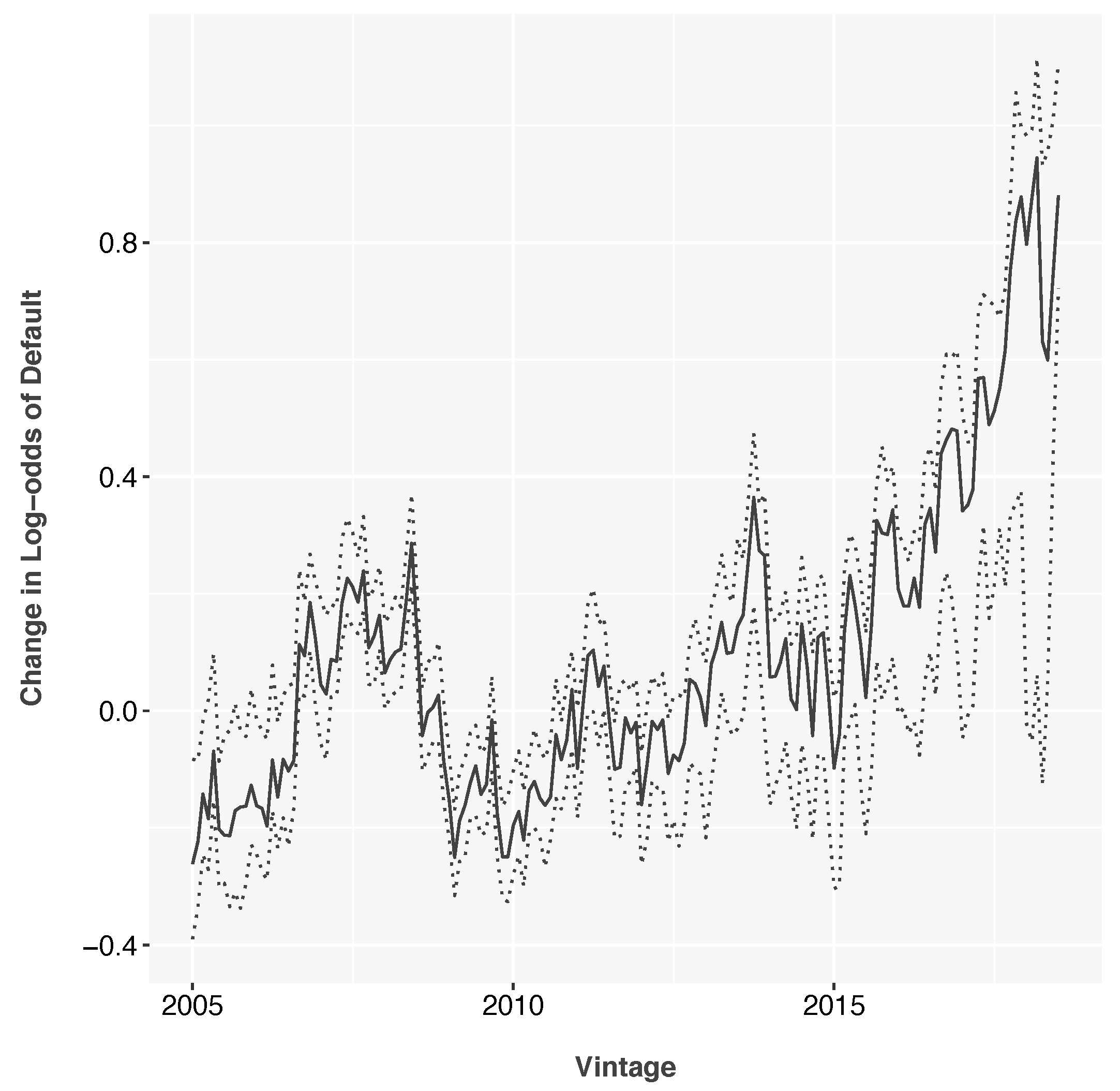
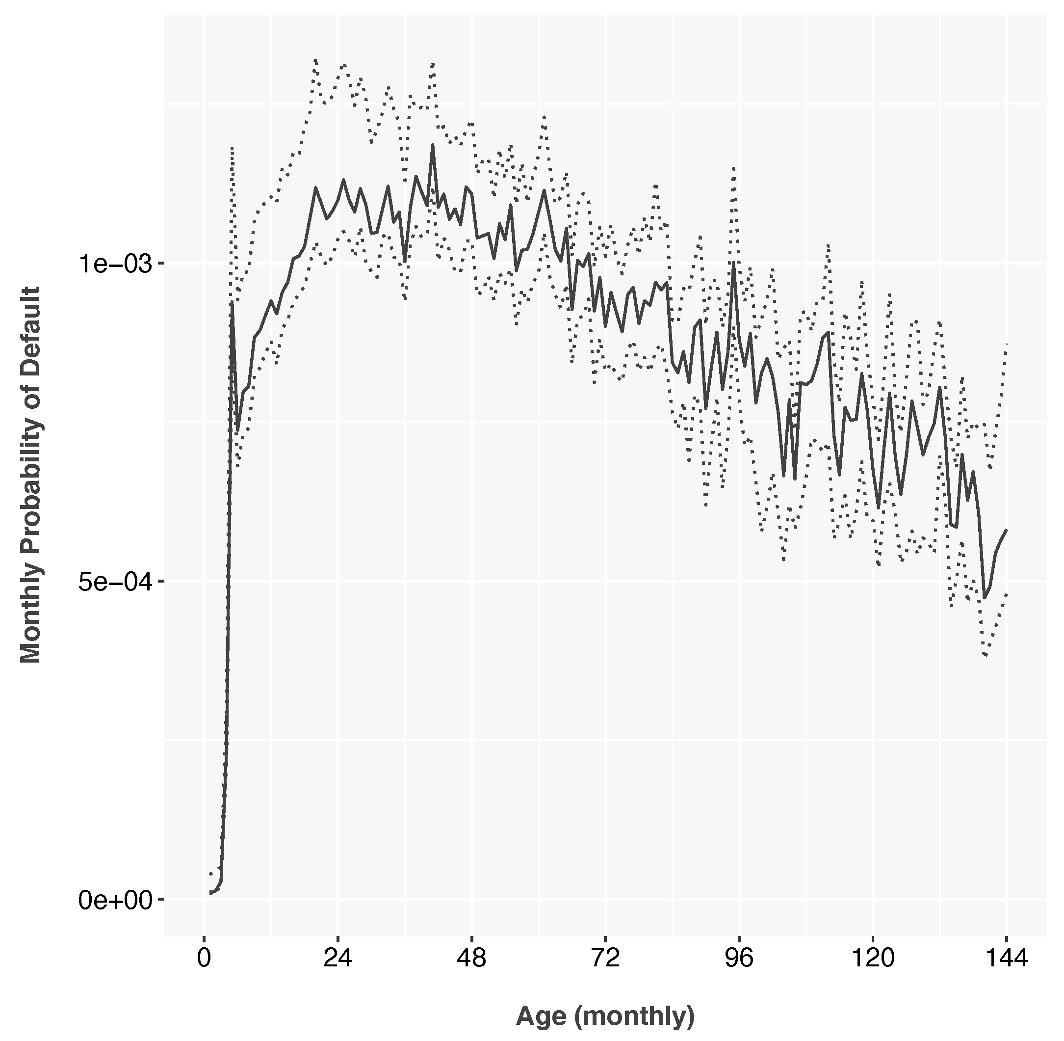
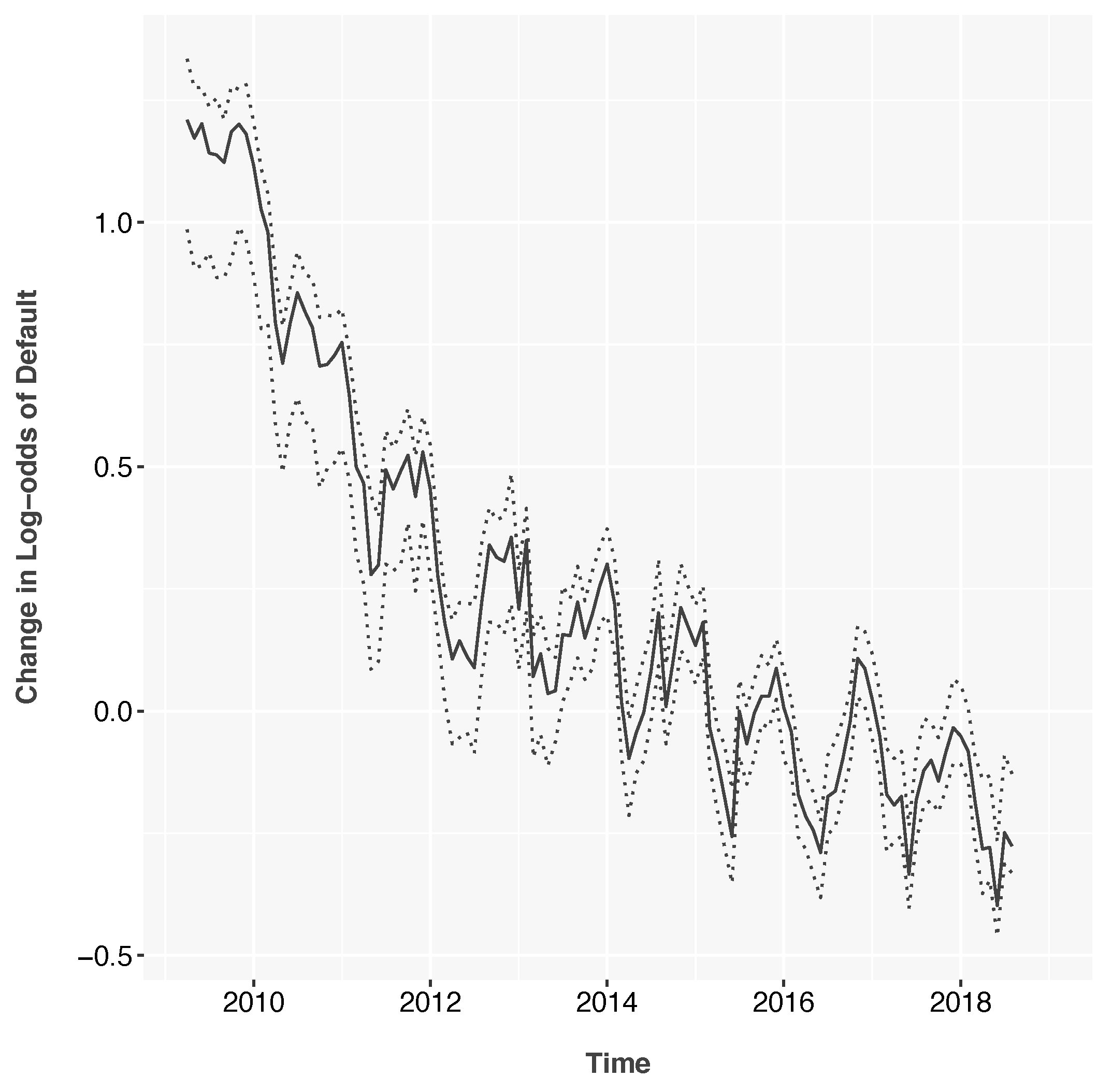
All the models created for this study begin with an age–period–cohort analysis of the data to normalize for trends due to product lifecycles and macroeconomic trends. Figure 1 and Figure 2 show the functions estimated on subprime credit card data.

The lifecycle function was estimated as log-odds of monthly default and then transformed to monthly probability of default for display purposes. It shows a peak risk around 36 months from origination and decreasing risk thereafter as the riskiest accounts have previously defaulted. The initial default spike represents fraud or other underwriting failures.

The vintage function shows the risk of each monthly vintage relative to the average lifecycle and is therefore centered about 0. This shows a risk peak in 2007–2008, as was common in the industry. The portfolio also shows rising risk in the most recent years, again, as has been seen in other portfolios. Both peaks could be a combination of macroeconomic adverse selection (Breeden and Canals-Cerdá 2018) and increased risk appetite by the lender.

The environment function, Figure 3 begins with the peak of the 2009 recession and shows steady macroeconomic improvement throughout history. Defaults also show a distinct seasonal pattern throughout history. Again, the environment function is measured relative to the lifecycle and is, therefore, mean zero.

The first scoring model estimated used the APC Scoring approach for logistic panel regression with standard credit risk inputs,

Table 2. Regression output from the APC Scoring model using standard credit risk modeling inputs.

Variable	Estimate	Std. Error	$\mathit{Pr}(>|\mathit{z}\left|\right)$
(Intercept)	1.06 $\times {10}^0$	2.29 $\times {10}^{-1}$	3.47 $\times {10}^{-6}$
original.score	−6.92 $\times {10}^{-4}$	8.45 $\times {10}^{-5}$	2.59 $\times {10}^{-16}$
loan.subcategoryGOLD	9.69 $\times {10}^{-1}$	2.20 $\times {10}^{-1}$	1.09 $\times {10}^{-5}$
loan.subcategoryPLATINUM	4.16 $\times {10}^{-1}$	2.11 $\times {10}^{-1}$	0.048867
loan.subcategoryPREFERRED	−2.80 $\times {10}^{-1}$	2.30 $\times {10}^{-1}$	0.223943
loan.subcategorySIGNATURE	−1.43 $\times {10}^0$	2.17 $\times {10}^{-1}$	4.22 $\times {10}^{-11}$
Credit.Limit (500, 2 $\times {10}^3$]	7.16 $\times {10}^{-2}$	7.65 $\times {10}^{-2}$	0.349463
Credit.Limit (2 $\times {10}^3$, 3 $\times {10}^3$]	1.67 $\times {10}^{-1}$	7.76 $\times {10}^{-2}$	0.031132
Credit.Limit (3 $\times {10}^3$, 5 $\times {10}^3$]	2.77 $\times {10}^{-1}$	7.25 $\times {10}^{-2}$	0.00013
Credit.Limit (5 $\times {10}^3$, 5.5 $\times {10}^3$]	4.39 $\times {10}^{-1}$	1.62 $\times {10}^{-1}$	0.006729
Credit.Limit (5.5 $\times {10}^3$, 7.5 $\times {10}^3$]	3.64 $\times {10}^{-1}$	8.23 $\times {10}^{-2}$	9.72 $\times {10}^{-6}$
Credit.Limit (7.5 $\times {10}^3$, 1 $\times {10}^4$]	5.09 $\times {10}^{-2}$	7.89 $\times {10}^{-2}$	0.519015
Credit.Limit (1 $\times {10}^4$, 1.15 $\times {10}^4$]	−6.44 $\times {10}^{-2}$	1.64 $\times {10}^{-1}$	0.695284
Credit.Limit (1.15 $\times {10}^4$, 1.5 $\times {10}^4$]	−3.12 $\times {10}^{-1}$	8.61 $\times {10}^{-2}$	0.000291
Credit.Limit (1.5 $\times {10}^4$, 7 $\times {10}^5$]	−2.64 $\times {10}^{-1}$	1.56 $\times {10}^{-1}$	0.091286
Credit.LimitNA	2.03 $\times {10}^{-1}$	7.98 $\times {10}^{-2}$	0.010954
Balance.Transfer (0, 9.96 $\times {10}^4$]	3.93 $\times {10}^{-2}$	1.02 $\times {10}^{-1}$	0.698951
Total.Loan.Balance (1 $\times {10}^3$, 1.19 $\times {10}^4$]	−3.51 $\times {10}^{-1}$	1.12 $\times {10}^{-1}$	0.001663
Total.Loan.Balance (1.19 $\times {10}^4$, 6.38 $\times {10}^4$]	−8.32 $\times {10}^{-1}$	1.07 $\times {10}^{-1}$	8.68 $\times {10}^{-15}$
Total.Loan.Balance (6.38 $\times {10}^4$, 2.19 $\times {10}^9$]	−6.31 $\times {10}^{-1}$	1.08 $\times {10}^{-1}$	5.14 $\times {10}^{-9}$
Total.Loan.BalanceNA	−5.21 $\times {10}^{-1}$	8.27 $\times {10}^{-2}$	3.03 $\times {10}^{-10}$
Total.Deposit.Balance (0, 79.6]	5.90 $\times {10}^{-1}$	7.10 $\times {10}^{-2}$	<2 $\times {10}^{-16}$
Total.Deposit.Balance (79.6, 732]	1.99 $\times {10}^{-1}$	5.39 $\times {10}^{-2}$	0.000223
Total.Deposit.Balance (732, 1.92 $\times {10}^3$]	−2.81 $\times {10}^{-1}$	6.52 $\times {10}^{-2}$	1.59 $\times {10}^{-5}$
Total.Deposit.Balance (1.92 $\times {10}^3$, 4.71 $\times {10}^3$]	−7.08 $\times {10}^{-1}$	7.99 $\times {10}^{-2}$	<2 $\times {10}^{-16}$
Total.Deposit.Balance (4.71 $\times {10}^3$, 1.67 $\times {10}^4$]	−8.78 $\times {10}^{-1}$	9.21 $\times {10}^{-2}$	<2 $\times {10}^{-16}$
Total.Deposit.Balance (1.67 $\times {10}^4$, 1.32 $\times {10}^8$]	−1.26 $\times {10}^0$	1.18 $\times {10}^{-1}$	<2 $\times {10}^{-16}$

. In a business application, credit limit would not be included as an input factor, because the score would be intended to advise the assignment of credit limits. In this retrospective analysis, credit limit highlights that some information was used in underwriting that was not otherwise available at the time of this retrospective.

Table 3. Coefficients for the APC Score built on restricted coefficients, part 1.

Variable	Estimate	Std. Error	Pr$(>|\mathit{z}\left|\right)$
(Intercept)	0.429434	0.496754	0.387325
Median.Age (33.1, 36.4]	−0.046453	0.063181	0.462201
Median.Age (36.4, 38.5]	−0.217667	0.068357	0.001451
Median.Age (38.5, 40.2]	−0.175815	0.070291	0.012376
Median.Age (40.2, 41.8]	−0.218958	0.074828	0.003432
Median.Age (41.8, 43.3]	−0.182989	0.077805	0.018678
Median.Age (43.3, 45]	−0.255418	0.084191	0.002415
Median.Age (45, 47.3]	−0.30382	0.094373	0.001285
Median.Age (47.3, 51.3]	−0.164469	0.102119	0.107276
Median.Age (51.3, 87.2]	−0.385565	0.110327	0.000475
Median.Age NA	−1.711184	1.200538	0.154057
MF.Ratio (0.883, 0.922]	−0.027993	0.060897	0.645749
MF.Ratio (0.922, 0.946]	−0.10739	0.062913	0.08783
MF.Ratio (0.946, 0.966]	−0.069961	0.0681	0.304265
MF.Ratio (0.966, 0.986]	−0.097892	0.07185	0.173055
MF.Ratio (0.986, 1.01]	−0.102649	0.076387	0.179013
MF.Ratio (1.01, 1.04]	−0.125782	0.083479	0.131872
MF.Ratio (1.04, 1.08]	−0.082608	0.093232	0.375594
MF.Ratio (1.08, 1.17]	0.012581	0.108319	0.907537
MF.Ratio (1.17, Inf]	−0.073213	0.128852	0.569905
Persons.Per.Household (2.15, 2.3]	−0.08188	0.085371	0.337503
Persons.Per.Household (2.3, 2.4]	−0.105344	0.085174	0.216155
Persons.Per.Household (2.4, 2.49]	−0.069261	0.086699	0.424368
Persons.Per.Household (2.49, 2.58]	−0.01589	0.085467	0.85251
Persons.Per.Household (2.58, 2.69]	−0.064099	0.086773	0.460087
Persons.Per.Household (2.69, 2.88]	−0.091609	0.085701	0.285096
Persons.Per.Household (2.88, 18.5]	−0.12349	0.090457	0.172196
Persons.Per.Household NA	2.198951	1.013411	0.030018
Asian.Frac (0.00129, 0.00249]	−0.084154	0.127895	0.510545
Asian.Frac (0.00249, 0.00383]	−0.227138	0.123017	0.064835
Asian.Frac (0.00383, 0.00578]	−0.074837	0.121216	0.536981
Asian.Frac (0.00578, 0.00868]	−0.049104	0.118761	0.679262
Asian.Frac (0.00868, 0.0139]	−0.033029	0.117145	0.77798
Asian.Frac (0.0139, 0.0252]	−0.119392	0.117556	0.309814
Asian.Frac (0.0252, 0.0544]	−0.211748	0.119053	0.075305
Asian.Frac (0.0544, 1]	−0.151513	0.122309	0.215429
Asian.Frac NA	−0.113808	0.247667	0.645861
Black.Frac (0.000733, 0.00279]	0.087864	0.436585	0.8405
Black.Frac (0.00279, 0.00481]	−0.318982	0.441355	0.469844
Black.Frac (0.00481, 0.00769]	0.067772	0.43275	0.875554
Black.Frac (0.00769, 0.0128]	−0.012755	0.431741	0.976431
Black.Frac (0.0128, 0.0241]	−0.056333	0.427847	0.895248
Black.Frac (0.0241, 0.0486]	−0.115476	0.426058	0.786365
Black.Frac (0.0486, 0.105]	−0.100944	0.425516	0.81248
Black.Frac (0.105, 0.251]	−0.160916	0.425417	0.705241
Black.Frac (0.251, 1]	−0.086803	0.425865	0.838489
Black.Frac NA	−0.671036	0.658327	0.308058

and

Table 4. Coefficients for the APC Score built on restricted coefficients, part 2.

Variable	Estimate	Std. Error	Pr$(>|\mathit{z}\left|\right)$
Native.American.Frac (0.00131, 0.00261]	0.052714	0.180282	0.769983
Native.American.Frac (0.00261, 0.00363]	0.126504	0.174445	0.468341
Native.American.Frac (0.00363, 0.00467]	0.215081	0.172942	0.213627
Native.American.Frac (0.00467, 0.00586]	0.184393	0.172979	0.286431
Native.American.Frac (0.00586, 0.00741]	0.279936	0.172713	0.105057
Native.American.Frac (0.00741, 0.00976]	0.278091	0.173732	0.109444
Native.American.Frac (0.00976, 0.0139]	0.204074	0.176386	0.247285
Native.American.Frac (0.0139, 0.0249]	0.231466	0.189609	0.222178
Native.American.Frac (0.0249, 1]	0.147134	0.199675	0.461205
Native.American.Frac NA	0.034517	0.405823	0.932218
Native.Hawaiian.Frac (0.000172, 0.000364]	−0.120674	0.08971	0.178575
Native.Hawaiian.Frac (0.000364, 0.00058]	−0.047631	0.087368	0.585634
Native.Hawaiian.Frac (0.00058, 0.000882]	−0.105189	0.087804	0.230916
Native.Hawaiian.Frac (0.000882, 0.00141]	−0.063272	0.088651	0.475399
Native.Hawaiian.Frac (0.00141, 0.00278]	−0.020393	0.090938	0.82256
Native.Hawaiian.Frac (0.00278, 0.832]	0.070064	0.103481	0.498361
Native.Hawaiian.Frac NA	−0.165063	0.112711	0.143062
Hispanic.Frac (0.00274, 0.0118]	−0.049692	0.202521	0.806173
Hispanic.Frac (0.0118, 0.0212]	−0.17317	0.200365	0.387436
Hispanic.Frac (0.0212, 0.0333]	−0.002096	0.198356	0.991569
Hispanic.Frac (0.0333, 0.0503]	−0.191075	0.197998	0.334527
Hispanic.Frac (0.0503, 0.0775]	−0.067762	0.196928	0.730773
Hispanic.Frac (0.0775, 0.131]	0.023131	0.197219	0.906634
Hispanic.Frac (0.131, 0.269]	0.101176	0.199284	0.611665
Hispanic.Frac (0.269, 1]	0.435275	0.204739	0.033503
Hispanic.Frac NA	0.138274	0.21503	0.520195

show the coefficients for the model built on restricted inputs. The coefficients of this model are marginally significant, but it is not subject to regulatory scrutiny, so we left everything in to maximize possible sensitivity.

The rest of the models were built using the same framework and variable sets as described previously.

Table 5. Descriptions of the models and forecasts created for testing.

In-Sample	Description
APC Scoring, Credit	Logistic regression on traditional credit scoring factors
	with APC lifecycle and environment as fixed inputs
APC Scoring, Restricted	Logistic regression on restricted census factors
	with APC lifecycle and environment as fixed inputs
APC Scoring, Credit with Restricted offset	Logistic regression on traditional credit scoring factors
	with the Restricted model and APC lifecycle and
	environment as fixed inputs
APC Scoring, Credit with Restricted = 0	The previous model with the Restricted model inputs
	set to 0 at the time of forecasting
APC + SGB, Credit with Restricted offset	Stochastic gradient boosted trees on traditional
	credit scoring factors with the Restricted model and
	APC lifecycle and environment as fixed inputs
APC + SGB, Credit with Restricted = 0	The previous model with the Restricted model inputs
	set to 0 at the time of forecasting

describes all of the models built and tested here.

6. Results

All the models were tested by creating 36-month forecasts from the origination date and using the actual lifecycle and environment as input. In a real-world test, the environment would be replaced with a macroeconomic model using macroeconomic scenarios as inputs. In the current context, macroeconomic models and scenarios are not germane to the topic of unintended bias.

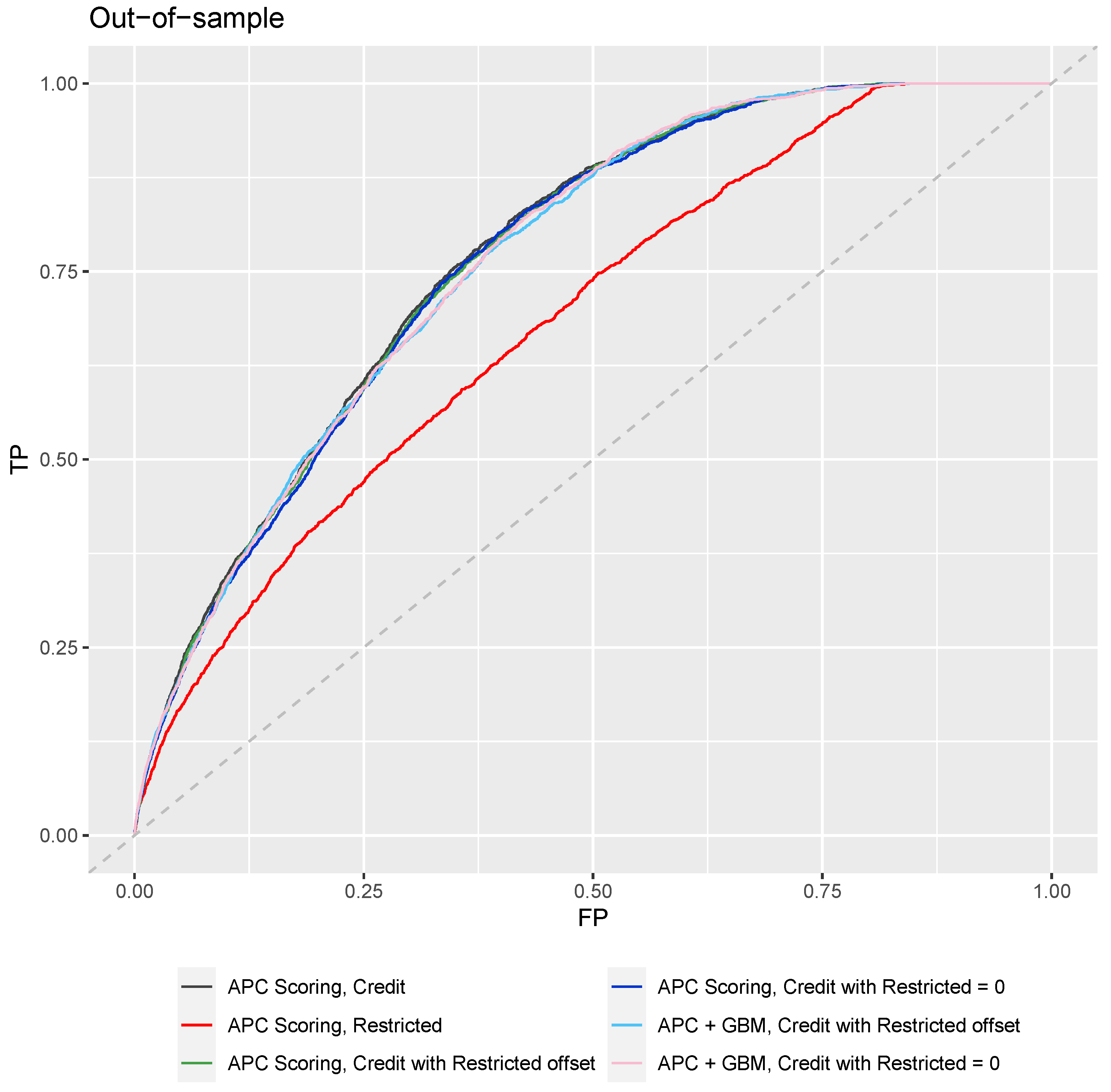
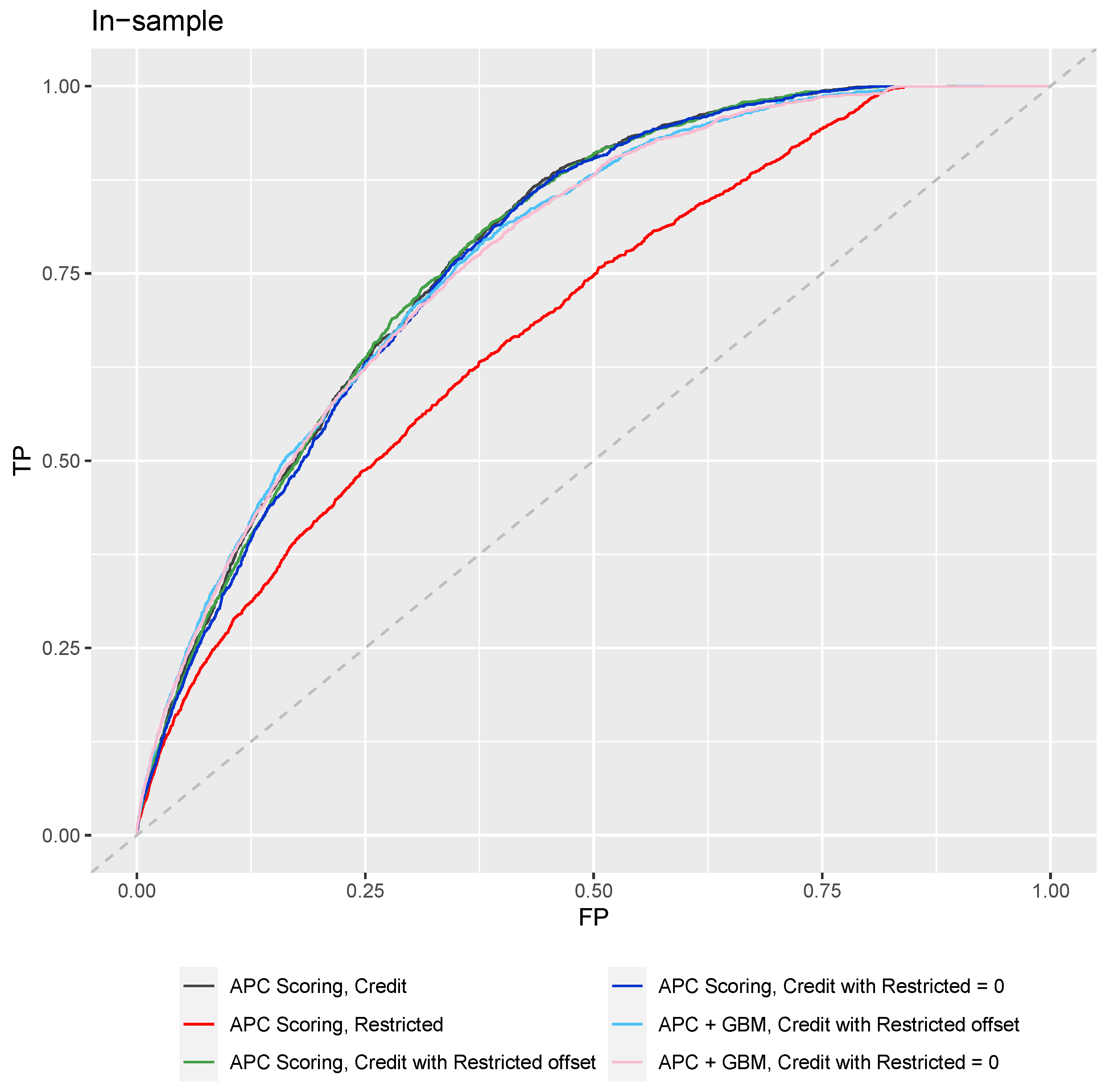
ROC curves are shown in Figure 4 and Figure 5, which are cumulative over the 36 month period for both forecasted and observed defaults. AUC and Gini coefficients were estimated from the ROC analysis, as shown in

Table 6. AUC and Gini coefficients for each of the models tested cumulatively over a 36-month forecast on the in-sample data set.

In-Sample	AUC	Gini
APC Scoring, Credit	0.783	0.565
APC Scoring, Restricted	0.689	0.379
APC Scoring, Credit with Restricted offset	0.782	0.564
APC Scoring, Credit with Restricted = 0	0.777	0.555
APC + SGB, Credit with Restricted offset	0.777	0.555
APC + SGB, Credit with Restricted = 0	0.775	0.550

and

Table 7. AUC and Gini coefficients for each of the models tested cumulatively over a 36-month forecast on the out-of-sample data set.

Out-of-Sample	AUC	Gini
APC Scoring, Credit	0.772	0.544
APC Scoring, Restricted	0.683	0.366
APC Scoring, Credit with Restricted offset	0.769	0.538
APC Scoring, Credit with Restricted = 0	0.767	0.533
APC + SGB, Credit with Restricted offset	0.767	0.533
APC + SGB, Credit with Restricted = 0	0.767	0.534

for in-sample and out-of-sample results, respectively.

The model built from restricted inputs alone is immediately less predictive than those using financial inputs. This is almost certainly due to the weak association between census data and the performance of an individual borrower, and because previous borrower performance in repaying debt really is the best predictor of future performance. We knew, going into this analysis, that census data was not sufficient to completely test unintended bias in a portfolio, but as a proxy, it serves to demonstrate the process.

Note that the forecast results degrade only slightly when the Restricted model is set to zero for forecasting. With actual borrower demographics, this degradation would probably be significantly increased. Comparing the models with the Restricted inputs and with those set to zero provides a quantitative comparison of the cost to lenders and society of enforcing our ethical standards. Just like clean water and safe roads, society should pay these costs to create the world we would wish to live in. This analysis simply provides a way to quantify that investment.

The results show only slight degradation when moving to out-of-sample performance. This has been observed previously in the context of building a score with APC lifecycle and environment as fixed inputs and is theorized to be due to the normalization provided by those inputs.

We also note that APC Scoring and APC + SGB Trees have nearly identical results. This is easily explained by considering the available credit scoring inputs. By binning the input data, the logistic regression of APC scoring is able to match the nonlinearity of stochastic gradient-boosted trees. Furthermore, the inputs are so simple that no important interaction terms are present. With a more complex data set containing many more interaction terms, we would expect APC + SCB trees to exhibit an advantage.

Furthermore, due to the relative simplicity of the available data, we chose not to test additional training methods such as artificial neural networks, but previous work (Breeden and Leonova 2019) has shown how neural networks can also be structured to utilize fixed inputs as needed to implement this approach to removing ethical bias.

7. Conclusions

This paper develops a modeling procedure that can create theoretically unbiased models so long as the training data are tagged with the protected class status against which one wants to prevent bias. The procedure is admittedly quite simple and yet highly effective. Most importantly, it avoids processes that have been shown to violate FCRA regulations, such as renormalizing the forecasts after model creation. We also find side benefits such as being able to quantify how much forecast accuracy is given up in the process of becoming provably unbiased. This was observed by comparing the forecast accuracy of the initial model with no fairness constraints to the model built with the restricted model as an input and then set to zero for testing. The difference in accuracy between two such models using any machine learning technique is a measure of the cost of creating an unbiased outcome. For the examples shown here, the difference between the initial model and the fully unbiased model was not statistically significant, but in other contexts and with other machine learning algorithms, it could be.

The application to a subprime credit card portfolio was effective because of the high default rate in the data and having a significant population of borrowers whom we wish to protect from discrimination. Combining borrower data with zipcode level census rates was not guaranteed to work, but the data actually showed plenty of useful structure.

The best test of this procedure will be to consider actual borrower demographic characteristics. If such data sets are not available in lending, perhaps applications outside lending would provide a safe and effective demonstration.