1. Introduction
Since the seminal works of
Dixit and Pindyck (
1994) and
Trigeorgis (
1996), it has become clear that real investments should be valued using a real options approach when decision makers are exposed to a significant amount of uncertainty. In these cases, the application of the standard net present value decision rule can lead to investment decisions that are significantly sub-optimal, as is extensively demonstrated in the above books. Since firm investment decisions lie at the basis of economic growth, it is crucial to take these decisions in the right way. From this perspective, it is clear that it is of main importance to work on the development of the theory of real options.
In a basic analysis, the real options model consists of a single firm, having the opportunity to invest in a project of given size, with revenue that is subject to uncertainty, being governed by a single stochastic process. Several authors have extended this framework in different directions.
Smets (
1991) was the first to consider a scenario where two firms can invest in the same market. The revenue in this market is still governed by one stochastic process, also, after both firms have already invested and, thus, are active in this market. The assumption “project of given size” is relaxed in
Bar-Ilan and Strange (
1999) and
Dangl (
1999), in which the firm not only needs to decide the time, but also the size of the investment.
Huisman and Kort (
2015) combine the two extensions by considering a duopoly market where both firms also have to determine the investment size.
For most real options, the literature uses a single (one-dimensional) stochastic process to model the evolution of random shocks affecting the investment’s value. This can be a major shortcoming, especially when analysing problems with, e.g., multiple firms or products. Such investment problems are especially common in the field of energy and environmental economics (
Agaton and Collera 2022;
Deeney et al. 2021;
Li and Cao 2022;
Zhang et al. 2021). The transition to a circular and low-carbon, bio-based economy requires firms to shift to the use of renewable resources, to cooperate with firms in other markets, and to valorize their waste streams (
The European Commission 2019,
2021). These decisions expose firms to different types of risks, creating the need for models that account for multiple sources of uncertainty. Therefore, in this paper, we consider a real options problem with multiple uncertain factors, which is an important extension to the basic real options analysis, especially from a practical perspective.
The first real options model with two-factor uncertainty occurs in
McDonald and Siegel (
1986). Their value function is homogenous of degree one, and the two stochastic processes are the output price and the investment cost. In such cases, the investment threshold level can be determined for the price-to-cost ratio. This allows to reformulate the problem in terms of the relative price, and to reduce the number of stochastic variables to one. In this way, a standard one-factor real options model is obtained for which a closed-form solution exists. The result of this analysis is, however, not a threshold point, but a threshold boundary at which it is optimal to invest (
Nunes and Pimentel 2017).
Hu and Øksendal (
1998) generalize this solution to the
n-dimensional case.
Armada et al. (
2013) consider a problem where the output price and quantity are stochastic. Here, the dimension of the state space can be reduced to a one-dimensional space, because the only relevant payoff variable is revenue (price times quantity). The problem then reduces to finding an optimal revenue threshold that makes investment optimal.
Several authors have tried to use this dimension reduction approach with cases characterized by multiple stochastic processes and a constant sunk cost.
Huisman et al. (
2013) and
Compernolle et al. (
2017) consider price and cost uncertainty and determine the investment threshold level for the price-to-cost ratio. However, there are some problems with this approach. In the presence of a constant sunk cost investment, homogeneity does not hold. For this reason, the state space cannot be reduced to a one-dimensional one. This is also revealed in these papers, because two processes (price/cost and cost) remain present in the equations.
For problems of this kind,
Adkins and Paxson (
2011b) propose a quasi-analytical approach that results in a set of equations to determine the optimal investment boundary. They solve this set of equations simultaneously while keeping one of the stochastic threshold variables fixed. The present paper shows that this methodology can lead to sub-optimal solutions. In fact, the results of the quasi-analytical approach will, generically speaking, be incorrect, and there is no guarantee that it converges in any meaningful sense to the correct solution. To put it succinctly, the main problem is that
Adkins and Paxson (
2011b) use a “local” approach to solve a “global” problem, which can lead to misleading results. Consequently, while the method is intuitively appealing and relatively easy to implement, we argue that care is required in checking that the results conform to economic intuition.
In this paper, we provide numerical examples for which the quasi-analytical approach violates certain properties of the optimal boundary that can be analytically established. The point is, in a nutshell, that when solving the partial differential equation that governs the value function, two power parameters turn out to be a function of the state variables, where the quasi-analytical approach starts with the assumption that these parameters are constant.
Our contribution to the literature is three-fold. Firstly, we alert the research community to potential pitfalls in a regularly used numerical method. In the literature, we find several papers concerning investment problems where the uncertainty is driven by multi-dimensional stochastic processes, and where no analytical solution can be derived. In such cases, the authors propose ways to circumvent the problem and come out with an approximation of the solution. For instance, we refer to
Kauppinen et al. (
2018), where the model proposed by
Adkins and Paxson (
2011b) is extended, by adding time to build to the investment problem. In the context of replacement options,
Adkins and Paxson (
2013a) examine a premature and postponed replacement in the presence of technological progress, where revenue and operating costs are treated as geometric Brownian motions.
Adkins and Paxson (
2017a) use a general replacement model to investigate when it is optimal to replace an asset whose operating cost and salvage value deteriorate stochastically.
The need to take into account multiple sources of uncertainty is also present in problems related with investments in the energy sector. For example,
Adkins and Paxson (
2011a) solve a switching model for two alternative energy inputs with fixed switching costs.
Boomsma and Linnerud (
2015) examine investment in a renewable energy project under both market and policy uncertainty.
Fleten et al. (
2016) study investment decisions in the renewable energy sector, where the revenue comes from selling electricity and from receiving subsidies, both stochastic.
Adkins and Paxson (
2016) consider the optimal investment policy for an energy facility with price and quantity uncertainty under different subsidy schemes.
Støre et al. (
2018) determine the optimal timing to switch from oil to gas production in the tail production phase, with the price of oil and gas following (correlated) Geometric Brownian motions. Finally, we refer to
Heydari et al. (
2012), who extend the quasi-analytical approach proposed in
Adkins and Paxson (
2011b) to a three-factor model, which is employed to value the choice between two emission reduction technologies, assuming that the value of each option depends on fuel, electricity and CO
2 prices, all following (correlated) Geometric Brownian motions.
Secondly, while it could, a priori, be the case that the approximation obtained by the quasi-analytical approach is close enough to the true solution to be of practical value, we show that for the models under consideration in much of the literature this is not necessarily the case. For example, in the model with two uncertain revenue flows, we find that in some situations the investment boundary decreases in an uncertainty environment. This violates one of the major qualitative results from real options theory: “an increase in uncertainty leads to an increase in project value”. We formally prove that this feature also holds for the model under consideration.
Thirdly, we develop a numerical algorithm which is based on a finite difference scheme and we apply this algorithm to a model with two stochastic revenue streams. We determine the optimal timing of investment in the presence of a constant sunk investment cost. Note that this model is different from the one analysed in
Adkins and Paxson (
2011b), who analyse a stochastic revenue and a (possibly correlated) stochastic cost. Importantly, our finite difference scheme
does exhibit the expected behaviour in relation to an increase in uncertainty.
In the literature, most finite difference schemes have been developed to solve models with a one-dimensional stochastic process and a finite time horizon. This method typically employs a backward induction argument in the time dimension to approximate the optimal exercise boundary and value function in a step-by-step fashion; see, e.g., (
Dixit and Pindyck 1994, Appendix 10.A). For a two-dimensional problem, this approach does not work, because both processes can move up or down in any time step. Therefore, we suggest a finite difference scheme that starts with a hypothesized boundary, after which the value function is approximated at all points in the two-dimensional finite grid at once. A discretized smooth pasting condition (in two dimensions) can then be used to judge the quality of the hypothesized boundary. This procedure is repeated until an acceptable approximation to the optimal boundary is found.
Note that to solve multidimensional optimal stopping problems, other numerical approaches could also be applied. Among the relevant contributions is
Lange et al. (
2020). In this paper, the authors consider that the decision to stop can only be taken at specific times, generated by an exogenous Poisson process with intensity rate
. This means that the set of admissible stopping times for the optimization problem is the set of events of a Poisson process, independent of the filtration generated by the state variables. In this setting, the optimization problem may be written as a fixed-point problem, for which the authors propose a numerical scheme, providing the proof and rate of convergence.
In our paper, we prove some analytical properties of the optimal boundary; notably, we prove that it is convex, non-increasing and continuous in
. In
Dammann and Ferrari (
2021), we may find similar results, but using different arguments that rely on a probabilistic representation of the Value Function. Moreover, the authors show that the boundary is the unique solution of an integral condition. By the use of this integral equation, they prove the monotonicity of the value function with respect to the the drift and volatility of the involved parameters. Finally, they propose a numerical approach to find the boundary, based on the integral equation using a Monte Carlo simulation.
The remainder of this paper is organized as follows:
Section 2 introduces a non-homogeneous investment problem characterized by two uncertain revenue flows.
Section 3 applies the methodological approach in
Adkins and Paxson (
2011b) to solve the model presented in
Section 2, and highlights the mathematical problems with the solution.
Section 4 proposes an alternative numerical approach to solve the model.
Section 5 concludes. Proof of propositions is presented in
Appendix A.
2. Investment Decision Given Two Uncertain Revenue Flows
Consider a profit-maximizing, risk-neutral firm that has the opportunity to invest in a production plant by paying a constant investment cost,
I. The plant can produce two different products, the prices of which are stochastic and follow correlated geometric Brownian motions
X and
Y, i.e.,
with
being the initial values of the processes
X and
Y, respectively. We noted that, in Equation (
1),
(
) denotes the drift of the process
X (
Y), whereas
(
) is the volatility of
X (
Y). Following the usual notation, we let
denote a standard two-dimensional Brownian motion, which we indexed by
X and
Y, respectively. We allowed these processes to be correlated so that
for some
, where
(
) means that
and
are positively (negatively) correlated.
At any instant, if the prices of the two products were
x and
y, respectively, then the instantaneous profit of the firm was given by:
where
and
denote the quantities of the products produced. Moreover, at that instant, the firm’s value was equal to the perpetual revenue flow from selling two products:
1
with
, and
r being the discount rate. To ensure finite integrals, we assumed that
. Equation (
4) gives the expected value of the discounted stream of profits that result from operating the production process forever, given current prices
x and
y. That is,
denotes the expectation operator, conditional on the initial state being
.
The firm needed to determine the optimal time to undertake the investment and, thus, solved the following optimal stopping problem:
where the supremum is taken over all stopping times
with respect to the filtration generated by the joint process
. That is, we were looking for the optimal time to invest in the production plant, given the current values for the price of each one of the two types of product, such that we maximized the expected value of the overall profit. By maximizing over stopping times, we recognized that the optimal time to invest may depend on the stochastic evolution of the product prices.
Using standard calculations from the optimal stopping theory (see, e.g.,
Øksendal and Sulem 2007), we derived the following Hamilton–Jacobi–Bellman (HJB) equation for this problem:
Here,
denotes the infinitesimal generator of the process
:
which is given by (
Øksendal and Sulem 2007):
This equation should be understood as follows: before the investment takes place, and assuming that the current prices of the products are x and y, the value of the firm, , is such that (and, thus, investment is not yet optimal) and that the optimality of the function V requires that . The latter equation essentially states that the investment’s value today is equal to the discounted expected value of the investment a short amount of time later. Then, as soon as investment is optimal, it holds that and that the value of immediate investment exceeds the discounted expected value of the investment a short amount of time later, i.e., .
Moreover, we let the set
denote the
continuation region, and
denote the
stopping region. Following the general theory of optimal stopping, it then follows that
, the time at which the investment should be undertaken, is given by the first exit time of the continuation region, i.e.,
Therefore, is the first time that the value function is equal to the expected value from immediately investing in the production plant.
In view of Equation (
6), it follows that:
The solution of the HJB equation,
V, must satisfy the following boundary condition:
which reflects the fact that the value of the firm will be zero if the prices are zero. Furthermore, the following value-matching and smooth-fit conditions should hold (see
Pham 1997;
Tankov 2003;
Alili and Kyprianou 2005):
Here, denotes the boundary of D, which we called the critical boundary, and ∇ is the gradient operator. Therefore, the solution of the problem is continuous at the critical boundary, not only for itself but also for its derivatives. The resulting threshold is a curve separating the two regions (the continuation and the stopping regions).
Note that
and
are absorbing barriers. Consequently, at these boundaries, the firm only receives revenues from one product and only one stochastic process is in use. Therefore, the threshold at these points corresponds to the standard solution for a one-dimensional problem. It follows that the investment triggers at the y and x axes are:
respectively. We refer, for instance, to
Dixit and Pindyck (
1994), for the derivation of these values.
These thresholds can be interpreted as follows: If
, then the firm should still invest in this plant as soon as the price of the other product reaches the value
. The intuition is analogous for
and
. The parameters
and
are the positive roots of the quadratic equations:
respectively.
Solving problem (
5) means, in particular, that we needed to derive the set of values for
x and
y where stopping was optimal, i.e., where investment should take place. In particular, we wanted to derive the boundary between
D and
S, as crossing this boundary meant that investment should be undertaken right away. We called it the
threshold boundary. As we had two state variables, we could define this threshold boundary as a surface in
, as follows: given that the price of one product is
, the firm should undertake the investment if the price of the other product is larger or equal to
. If it is smaller, then the firm should wait before investment. The next theorem derives some qualitative features of the threshold boundary for the problem defined in (
5).
Theorem 1. The boundary between D and S can be described by a mapping , where:
- 1.
for all ;
- 2.
b is non-increasing on ;
- 3.
b is convex on ;
- 4.
b is continuous;
- 5.
on , and on .
In addition, the stopping set S is:
Finally, the value function V satisfies:
- 1.
on ;
- 2.
V is convex;
- 3.
V is continuous;
- 4.
V is increasing in x and y.
Remark 1. Theorem 1 leads to the following observations.
- 1.
- 2.
The optimal stopping boundary can never lie below the Net Present Value boundary , i.e.,
Thus, in order to solve (
5), we needed to find
V and, at the same time,
for
, such that the properties enumerated in Theorem 1 held. In particular for
V, conditions usually known in the literature as
fit conditions were checked: the value-matching condition (for the continuity of the value function) and smooth pasting (for the smoothness of the value function).
3. The Quasi-Analytical Approach
Following the approach in
Adkins and Paxson (
2011b), we started by postulating a solution to Equation (
6) of the following form:
where
A,
, and
are constants. Simple calculations led to the conclusion that for (
14) to be a solution to (
7), it must hold that
and
are the roots of the characteristic root equation:
The set of solutions to (
15) defines an ellipse that intersects all quadrants of
, with
(
) on the horizontal (vertical) axis.
Adkins and Paxson (
2011b) hypothesize that the boundary between the continuation and stopping regions is of the form
. As Theorem 1 shows, this is correct. In order to find this boundary,
Adkins and Paxson (
2011b) try to extend the standard value-matching and smooth-pasting conditions to a two-dimensional setting. The way this is performed is as follows: on the boundary, it should hold for every
, with
as given in Equation (
13):
Now,
if the value function is of the form
2
then, it should hold that
since the boundary conditions
should be satisfied. Therefore, for every
we could solve the system of non-linear equations:
in
b,
A,
and
, under the condition that
.
Using the approach presented in
Støre et al. (
2018) to solve this system, we found the explicit solution for the boundary
3:
where
In the previous equations, we used and instead of and to emphasize the dependency on the state variable x.
Therefore, solving (
20)–(
22) led to values of
and
that
do depend on the value of
x and, thus, could not be treated as fixed parameters. This was also the case for the problem in
Adkins and Paxson (
2011b), as illustrated by their Figure 3.
4 The same held for
A and
b.
Let
denote the vector of solutions resulting from (
20)–(
22). Then at
, the value of the firm could be written as:
Note that from (
9), the partial differential equation
must also hold along the threshold boundary, implying that:
Using (
27) we could rewrite (
28) as:
The first two terms in (
29) represent the contributions of the partial derivatives of
,
A,
and
with respect to
x, whereas the last term is equal to
. If the solution proposed in (
14) is correct, then the latter should be equal to zero, and we could still use system (
19)–(
22) to determine the threshold boundary. In what follows, we verified whether the contribution of the partial derivatives was negligible for the numerical example in
Table 1.
For
, and the set of parameter values in
Table 1,
. Therefore, we concluded that the contribution of the partial derivatives could not be neglected. As a result, the substitution of the solution (
27) in (
7) led to the conclusion that the condition for
and
was no longer (
15). In fact, (
15) needed to be modified to incorporate terms involving
,
,
,
,
,
,
and
. The implication was that solving system (
19)–(
22) for different values of
would not result in a correct threshold boundary.
Results of the Quasi-Analytical Approach
After having shown that the boundary
, as determined by the quasi-analytical approach, is not the true boundary
b, it could still be the case that
is a good approximation of
b. This section, however, provides an argument that this was not the case, at least for the problem in
Section 2.
We started out by presenting the following proposition:
Proposition 1. The value function, V, is monotonically increasing in both and .
Proof. The result follows from Proposition 3 in
Olsen and Stensland (
1992), using the fact that the optimal value function is convex, as stated in our Theorem 1. □
In the following, we studied the behaviour of the investment boundary as a function of the volatilities of the involved processes, and . Thus, we let denote the boundary, given that the current price of the first product was x, and that the volatilities were (for X) and (for Y).
Corollary 1. Let denote the optimal investment threshold boundary for a given level of x. Then, it holds that is increasing in both and .
Proof. We proved the result by contradiction. Without the loss of generality, we only considered a change in
. Consider two different values of
, such that
, and
for some
x. Let
denote the optimal value function for a given level of
x. Then,
If , then for , it holds that , which contradicts Proposition 1. □
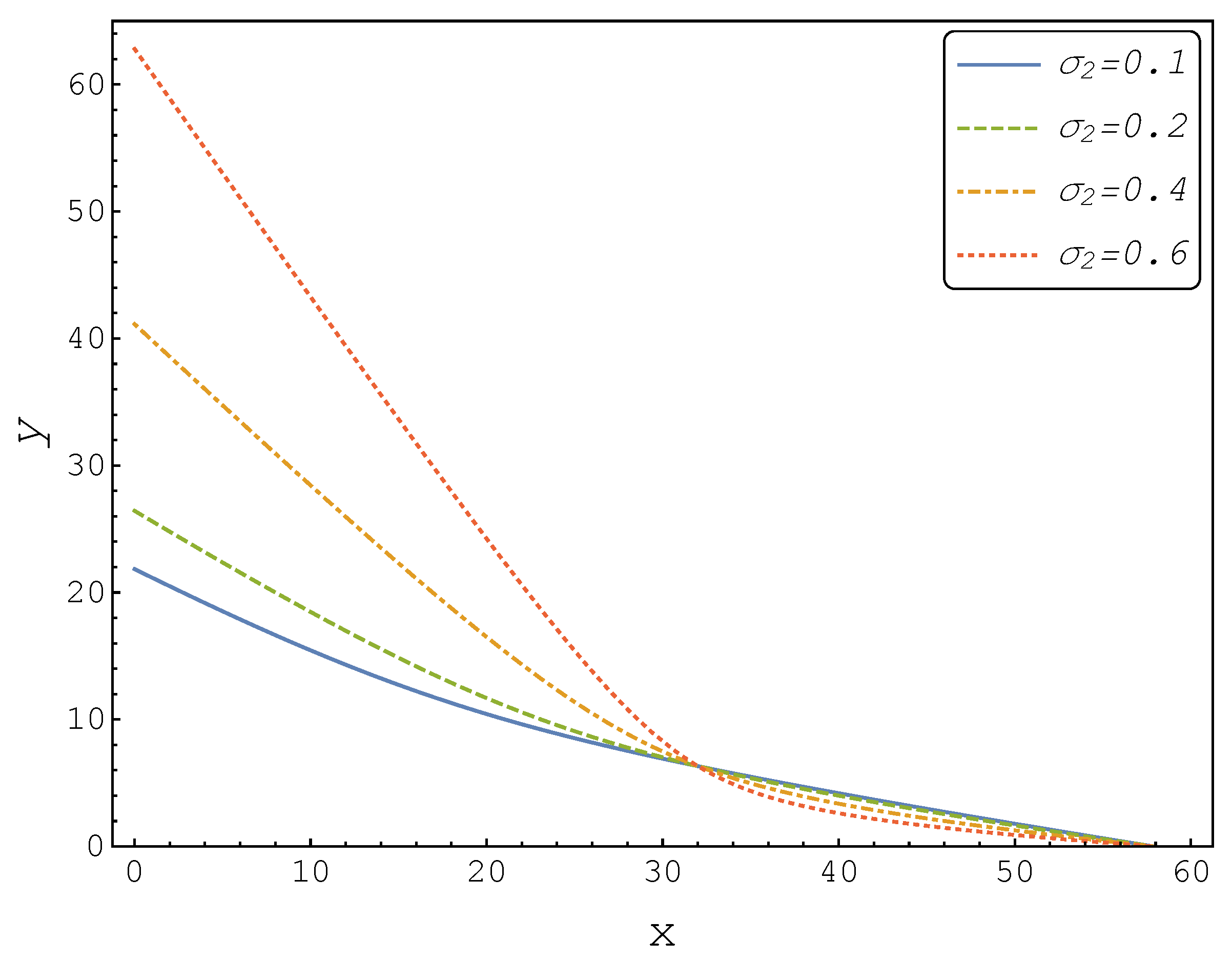
Figure 1 illustrates the quasi-analytical threshold boundaries for different values of
.
Evidently, the numerical example violated Corollary 1, since the threshold boundaries intersected. Moreover, this result did not correspond to what we would expect from a real options theory, i.e., that the firm invests for a larger threshold level in a more uncertain environment. In fact, for , the quasi-analytical approach suggested that the firm should invest for a lower threshold level when was larger. This clearly led to a sub-optimal decision, so the quasi-analytical solution fell short in being a useful approximation to the optimal solution in this case.
4. Numerical Solution
This section developed a finite difference algorithm to solve the optimal stopping problem in (
5). The results of the numerical approach were different from the results obtained by the analytical approach
in line with Theorem 1 and Proposition 1.
We started by generating a discrete grid over the domain of the partial differential equation in (
7). Thus, we assumed that the intervals
and
were divided in
and
equally spaced subintervals, respectively, and we let:
where
and
are the optimal investment triggers in case the other state variable is zero and, thus, are the natural end points of the grid. Moreover, we considered the following notation:
denotes the value of the firm at the grid points
:
with
V defined in Equation (
5). Finally, we let
be the vector of unknown grid points, which could be ordered in the following way:
Then, we were able to derive a linear system of equations that allowed to solve for the discrete grid points simultaneously, as follows: We discretized the partial differential equation using a weighted sum of the function values at the neighbouring point approximations to the partial derivatives. This yielded:
Rearranging the terms, gave:
Then, the partial differential Equation (
35) could be represented as a system of linear equations:
where
B is the matrix of coefficients resulting from (
36).
This system could be solved by applying appropriate boundary conditions. We used the fact that the value at
and
had to equal the value of the immediate investment. In addition, if either
or
was equal to zero, the problem was reduced to one dimension, and the grid points together with the threshold boundary could be found analytically. Given a candidate threshold function, system (
37) in combination with the boundary conditions in zero and final nodes, yielded a solution for the unknown grid points. To determine the optimal threshold, we implemented the following procedure: First, we proposed a shape of the exercise boundary. For example, the results that we presented in
Figure 2 were based on the quadratic function, i.e.,
. The unknown parameters,
a and
b, could be determined using the analytical threshold boundaries when either
or
was zero. In order to find
c, we computed the derivative of the option value at the candidate threshold boundary at each node and compared it with the derivatives resulting from the smooth-pasting conditions. Next, we computed the sum squared error of the differences and minimized it with respect to unknown parameter
c, which allowed to determine the optimal threshold in such a way that the smooth-pasting condition was satisfied.
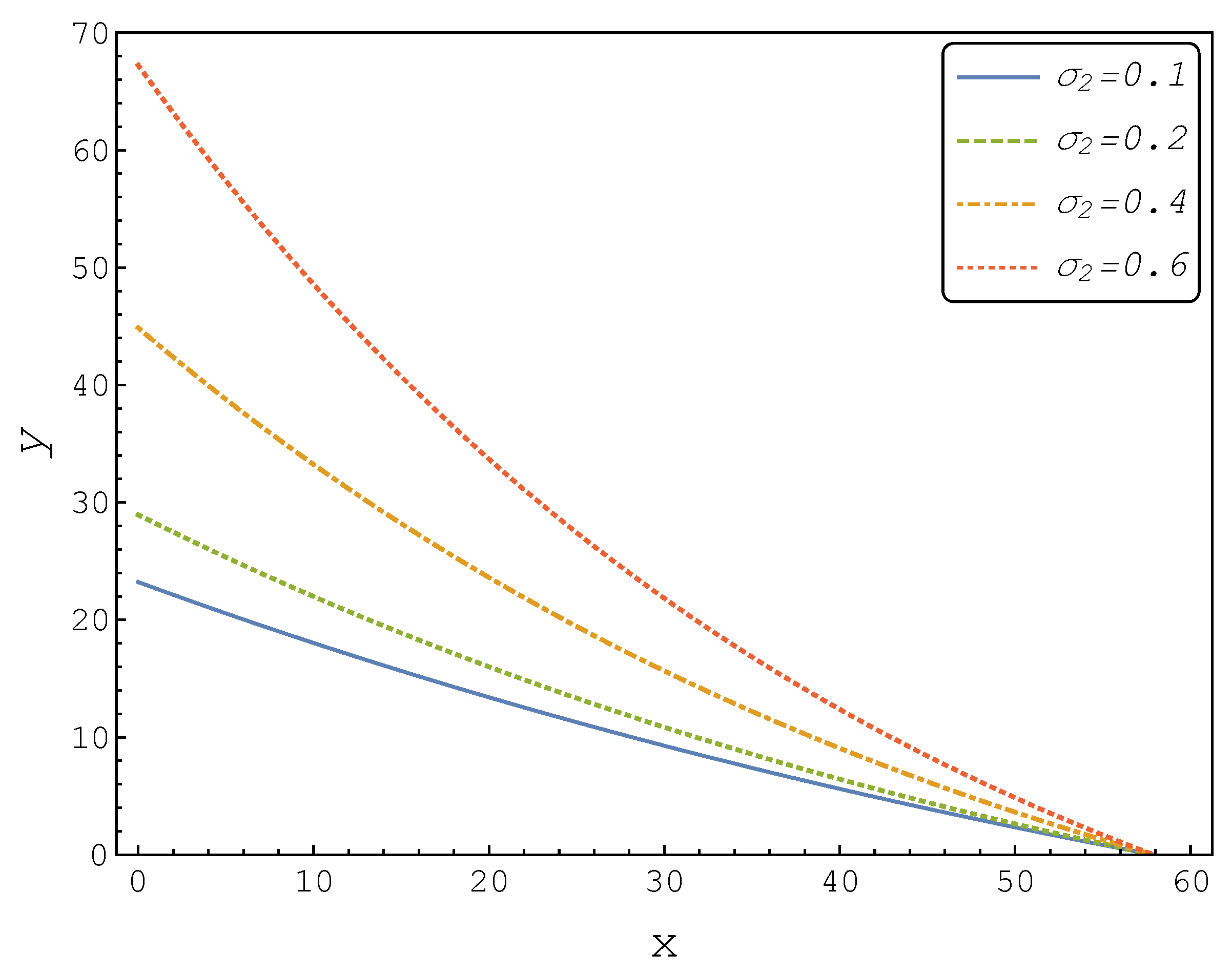
We now replicated
Figure 1 using our finite difference scheme and depicted it in
Figure 2.
This numerical example resulted in a more intuitive shape of thresholds boundaries and represented a standard result from the real options theory. Namely, an increase in volatility led to an increase in the optimal investment threshold.
In addition, finite difference also allowed for the calculation of an approximation to the value function that was implied by the quasi-analytical boundary
. This could be performed by solving (
37) for the boundary in (
23).
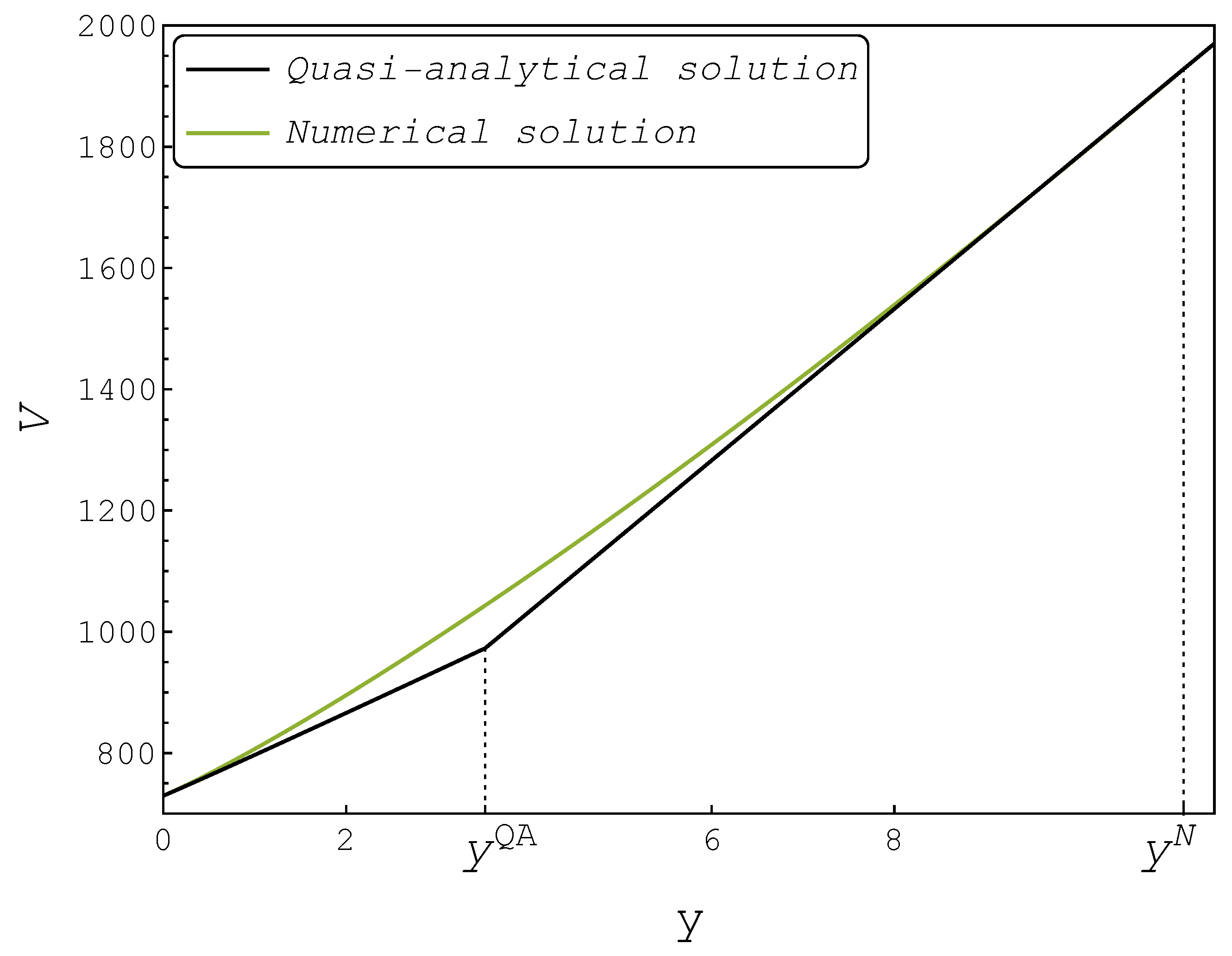
Figure 3 illustrates the comparison between the implied value function and the numerical solution represented by the quadratic boundary for a fixed level of
x and different values of
y.
From
Figure 3, it is evident that the value function implied by the quasi-analytical solution had a kink at the boundary point
, violating the smooth-pasting condition. Consequently, the quasi-analytical approach underestimated the true value function, which led to a sub-optimal investment decision rule for large values of
x. Note that the quasi-analytical approach suggested a much lower trigger than our finite difference scheme. For
, the numerical procedure based on the finite difference algorithm gave the boundary point
, such that the smooth-pasting condition held.
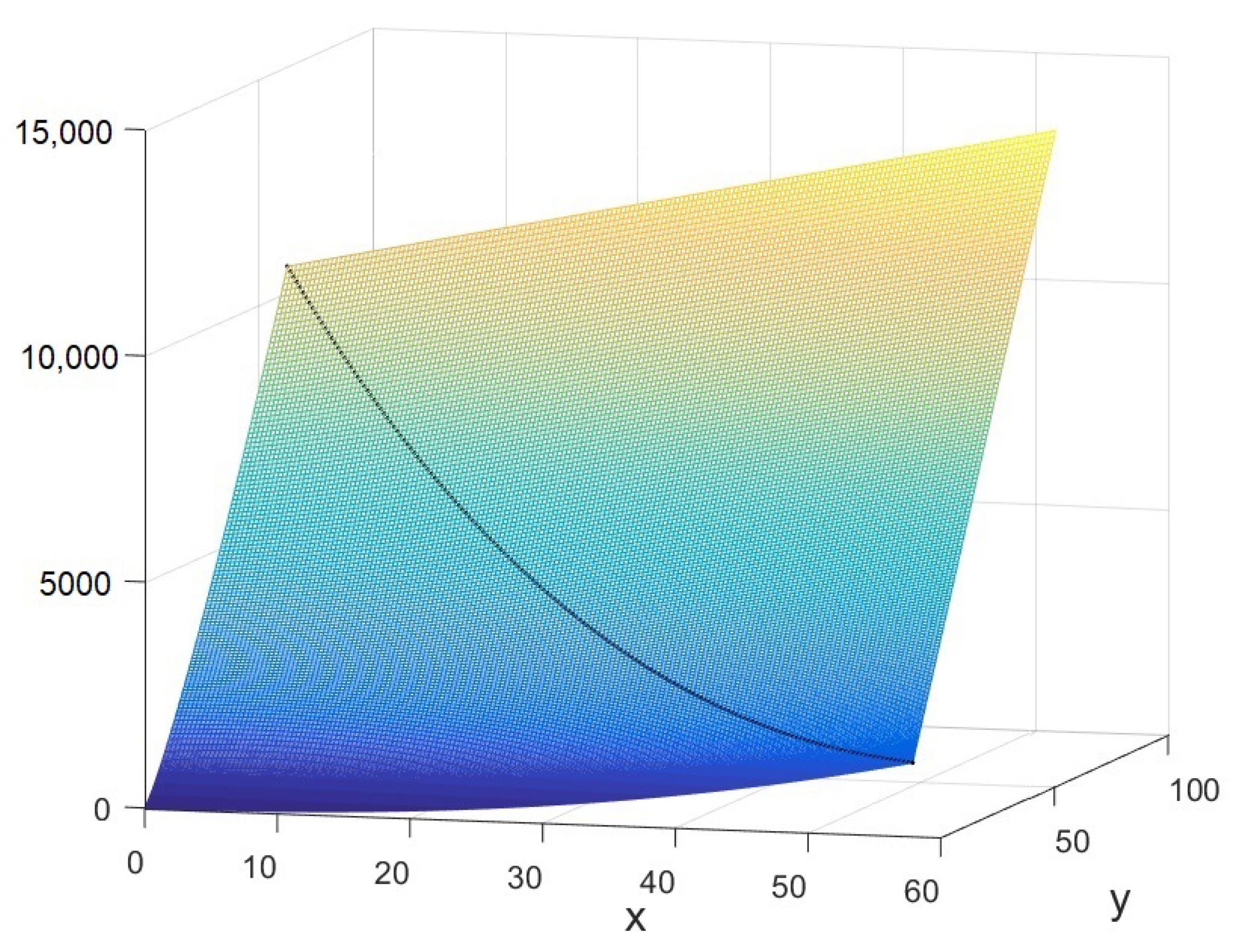
Figure 4 illustrates the value function for different values of
x and
y, as well as the threshold boundary.
As can be seen, the value appeared to be smooth for different values of x and y in the grid. The average squared error resulting from the numerical procedure was equal to 0.44, which corresponded to of the true value of the total derivative of the value function. Therefore, we concluded that the proposed numerical method was a good approximation for the true value function and optimal threshold.
Lastly, in order to give an indication of how often a firm would make a poorly timed investment decision, we simulated the passage time for processes
and
to reach the quasi-analytical boundary. We then ran the procedure 5000 times for a specific set of starting values
, and calculated the percentage of cases of the threshold being reached within the next 5 years. We performed a similar procedure to determine the investment probabilities for our numerical solution. The results for the different starting points are presented in
Table 2.
Table 2b shows that, for example, for the starting values (15,10), the firm should invest in 5.41% of the cases. According to the quasi-analytical approach, however, the firm invests in 42.87% of the cases, implying that the firm invests many times, while it is in fact not optimal to do so.
5. Conclusions
This paper developed an easy-to-implement finite difference algorithm to solve real options models with two-factor uncertainty. The proposed framework is, thus, highly relevant for the evaluation of business opportunities involving multiple end-products, a switch in feed-stock or end-product, a cooperation between firms that are operative in different markets and investments in new technologies incentivized by market-based policy instruments.
We applied it to a particular investment problem, where, after investment, the firm was able to produce two different products. The output prices of these products followed two geometric Brownian motion processes, possibly correlated. The investment cost was constant and sank. We contrasted our solution approach to the quasi-analytical approach developed by
Adkins and Paxson (
2011b) to address such problems. The latter has already been adopted by several other authors, as the overview in
Section 1 showed. This paper argued, however, that this quasi-analytical method does not always result in the correct investment decision rule.
From the analysis of this two-factor real options problem, we obtained that the quasi-analytical investment decision rule in some cases also failed to be a reasonable approximation to the optimal decision. In particular, we found that the quasi-analytical solution did not comply with the (analytical) result that the investment threshold boundary had to be monotonically increasing in the volatility parameters of both stochastic processes.
The ultimate conclusion was that non-homogenous real options problems with two-factor uncertainty should be solved using a different numerical procedure, or at the very least, the quality of the quasi-analytical approximation should be discussed. Note, however, that if our two-factor uncertainty problem was homogenous, then a standard (cf.
McDonald and Siegel 1986) reduction in dimensionality could be obtained, leading to an analytical solution.

 ,
, 


