Univariate and Multivariate Machine Learning Forecasting Models on the Price Returns of Cryptocurrencies

Abstract

In this study, we predicted the log returns of the top 10 cryptocurrencies based on market cap, using univariate and multivariate machine learning methods such as recurrent neural networks, deep learning neural networks, Holt’s exponential smoothing, autoregressive integrated moving average, ForecastX, and long short-term memory networks. The multivariate long short-term memory networks performed better than the univariate machine learning methods in terms of the prediction error measures.

1. Introduction

Cryptocurrencies are virtual currencies used to buy goods and services; there is no need for financial institutions such as central authorities or clearing houses in transactions involving cryptocurrency. Bitcoin was the first cryptocurrency, created back in 2009, and since Nakamoto (2008), there have been over several thousand alternative cryptocurrencies. Prior research extensively studied Bitcoin for hedging and diversification benefits. Shahzad et al. (2021) found that Bitcoin is appealing for diversification purposes for hedge assets in BRICS (Brazil, Russia, India, China, and South Africa) stock markets. Wang et al. (2019) also found that cryptocurrency is a hedge or a safe haven for international indices. Kim et al. (2020) also studied the relationship of cryptocurrency prices with US stock and gold prices using copula models. The value of cryptocurrencies has also skyrocketed over the years, making it an emerging market for investors wanting to capitalize on the daily fluctuations of cryptocurrencies. There have been numerous studies on understanding the volatility of cryptocurrencies. Katsiampa (2017) studied volatility estimation for Bitcoin by comparing generalized autoregressive conditional heteroskedasticity (GARCH) models. Katsiampa (2019) also conducted an empirical investigation of volatility dynamics in the cryptocurrency market. Phillip et al. (2019) studied long memory effects in the volatility measure of cryptocurrencies. Mostafa et al. (2021) implemented GJR-GARCH over the GARCH model to estimate the volatility of 10 popular cryptocurrencies based on market capitalization: Bitcoin, Bitcoin Cash, Bitcoin SV, Chainlink, EOS, Ethereum, Litecoin, TETHER, Tezos, and XRP. Kim et al. (2021) used stochastic volatility and GARCH models on cryptocurrencies that they selected for the study, and learned that the stochastic volatility method has better forecasting results compared to the GARCH method.

To accurately forecast future cryptocurrency prices, Akyildirim et al. (2021) predicted the 12 most liquid cryptocurrencies by using machine learning classification algorithms such as support vector machines, logistic regression, artificial neural networks, and random forests. Plakandaras et al. (2021) applied different methodologies—such as ordinary least squares (OLS) regression, support vector regression (SVR), and least absolute shrinkage and selection operator (LASSO) techniques—from the field of machine learning to predict the price of cryptocurrency. Hyun et al. (2019) invested the directional dependence structure among top volume cryptocurrencies by using copula and neural networks models.

In this study, we apply univariate and multivariate machine learning methods such as recurrent neural networks (RNNs), deep learning networks (DNNs), long short-term memory networks (LSTMs), Holt’s exponential smoothing, autoregressive integrated moving average, and ForecastX to predict the log returns of cryptocurrencies. We selected the top 10 cryptocurrencies based on a measure known as market capitalization, which refers to the total value of a cryptocurrency. This paper is organized as follows: Section 2 presents the summary and graphical data analysis for the top 10 cryptocurrencies. Section 3 gives an overview of the machine learning models used in this study. The illustrated comparison study for the proposed methods will be performed in terms of the measures of errors in Section 4, and the conclusion in Section 5.

2. Study Design and Data Collection

The cryptocurrency data used in this study were attained from an API known as CryptoCompare—a package in Python. The variables for each of the cryptocurrency datasets before manipulation were low, open, time, high, volume from, volume to, conversion type, conversion symbol, and close. The end date for each of the 10 cryptocurrencies was 14 July 2021. Bitcoin (BTC), Ethereum (ETH), Ripple (XRP), Tether (UDST), and Dogecoin (DOGE) had a start date of 1 January 2017. Binance Coin (BNB) had a start date of 15 August 2017. Cardano (ADA) had a start date of 10 October 2017. FLOW (FLOW) had a start date of 29 January 2021. USD Coin (USDC) had a start date of 11 October 2018. Uniswap (UNI) had a start date of 18 September 2020. Let $S_t$ be a price time series at time t; for a log return series, ${\mathrm{r}}_{\mathrm{t}}=log\left(\frac{S_t}{S_{t-1}}\right)$. Each of the cryptocurrency datasets was given a new variable, known as log returns. We summarized descriptive statistics of log return data of cryptocurrency, such as mean, skewness, and kurtosis, as well as five summary statistics, as shown in

Table 1. Summary statistics of the top 10 cryptocurrencies.

	Size	Mean	SD	Min	Q1	Median	Q3	Max	Kurtosis	Skewness
BTC	1654	0.002	0.044	−0.480	−0.016	0.003	0.022	0.228	11.016	−0.811
ETH	1654	0.003	0.058	−0.570	−0.023	0.002	0.031	0.260	8.165	−0.483
USDT	1654	0.000	0.046	−0.693	−0.001	0.000	0.001	0.454	77.596	−2.135
XRP	1654	0.003	0.079	−0.653	−0.027	−0.001	0.024	1.028	28.286	1.868
BNB	1423	0.004	0.072	−0.566	−0.026	0.001	0.032	0.533	11.162	0.325
ADA	1382	0.003	0.076	−0.539	−0.032	0.001	0.034	0.862	20.509	1.734
FLOW	167	0.006	0.092	−0.362	−0.042	−0.003	0.043	0.367	3.057	0.464
USDC	1008	0.000	0.002	−0.011	−0.001	0.000	0.001	0.020	17.396	1.571
DOGE	1654	0.004	0.088	−0.601	−0.025	−0.001	0.023	1.594	71.995	4.226
UNI	300	0.005	0.092	−0.408	−0.047	−0.002	0.050	0.501	5.082	0.730

Note: Size is the sample size, SD is the standard deviation, Min is the minimum, Q1 is the first quartile, Q3 is the third quartile, and Max is the maximum.

. Table 1 shows the summary statistics for each of the cryptocurrency datasets.

In Table 1, it is recognized that the standard deviation of BTC is smaller than those of ETH, USDT, XRP, BNB, ADA, FLOW, DOGE, and UNI (all of the listed cryptocurrencies except for the stable cryptocurrency USDC), which means that BTC has a lower risk than other cryptocurrencies in terms of investment. In addition, the values of kurtosis in the log returns of all cryptocurrencies in Table 1 are greater than 3, meaning heavy tails compared to normal distribution. The BTC, ETH, and USDT are left-skewed, while XRP, BNB, ADA, FLOW, USDC, DOGE, and UNI are right-skewed. UNI and FLOW have the lowest counts due to how new they are compared to BTC, ETH, USDT, XRP, and DOGE, which have the highest counts. In terms of the median for log returns, BTC, ETH, BNB, and ADA have positive values.

Figure 1 visualizes the boxplot of price log returns for each of the cryptocurrencies. The value for USDC seems to be around zero because USDC is a stable cryptocurrency, whereas the values of price log returns for XRP, BNB, USDT, ADA, and DOGE are more scattered around the zero because most of the Altcoins have a high volatility. The values of price log returns for BTC, ETH, and FLOW are less volatile than those of XRP and DOGE in Table 1.

Figure 2 visualizes each of the cryptocurrency price log returns over time. This allows us to understand the volatility of the cryptocurrencies. The cryptocurrency price log returns are shown to be volatile due to their frequent fluctuations over time. The cryptocurrency price log returns show a similar pattern of hitting at least one all-time high or low. FLOW is the only cryptocurrency that has a date value of just 2021. When looking at how the log returns of FLOW compare to the log returns of other cryptocurrencies in the predictions, the lack of data may affect the performances of models predicting cryptocurrencies’ price log returns.

Figure 3 shows a heat map of the relationships between the price log returns of cryptocurrencies. BTC and USDT are the only cryptocurrencies that have mostly negative correlations with the other cryptocurrencies in terms of price log returns. This may be due to USDT being a stable cryptocurrency, so when the prices of BTC or other Altcoins collapsed, investors moved to the stable cryptocurrency to hedge their investment in the cryptocurrencies. The other cryptocurrencies have moderate correlation with one another. This may suggest that the multivariate machine learning model known as long short-term memory networks may be useful in predicting the price returns of cryptocurrencies.

3. Statistical Methods

In this paper, we compare the forecasting prediction accuracy for the price log returns of cryptocurrencies by employing both conventional univariate time-series models and machine learning time-series models. We also used Python to forecast the price log returns of cryptocurrencies and find whether the univariate and multivariate machine learning methods such as RNN, DNN, Holt’s exponential smoothing, ARIMA, ForecastX, and LSTM are useful in predicting the price log returns of cryptocurrencies. Python is a programming language used through an integrated development environment known as Spyder. An RNN is an artificial neural network with multiple layers that depend on prior elements in the sequence between the input and output layers. A DNN is an artificial neural network with multiple layers between the input and output layers. An LSTM is a type of RNN that can account for learning long-term temporal dependencies.

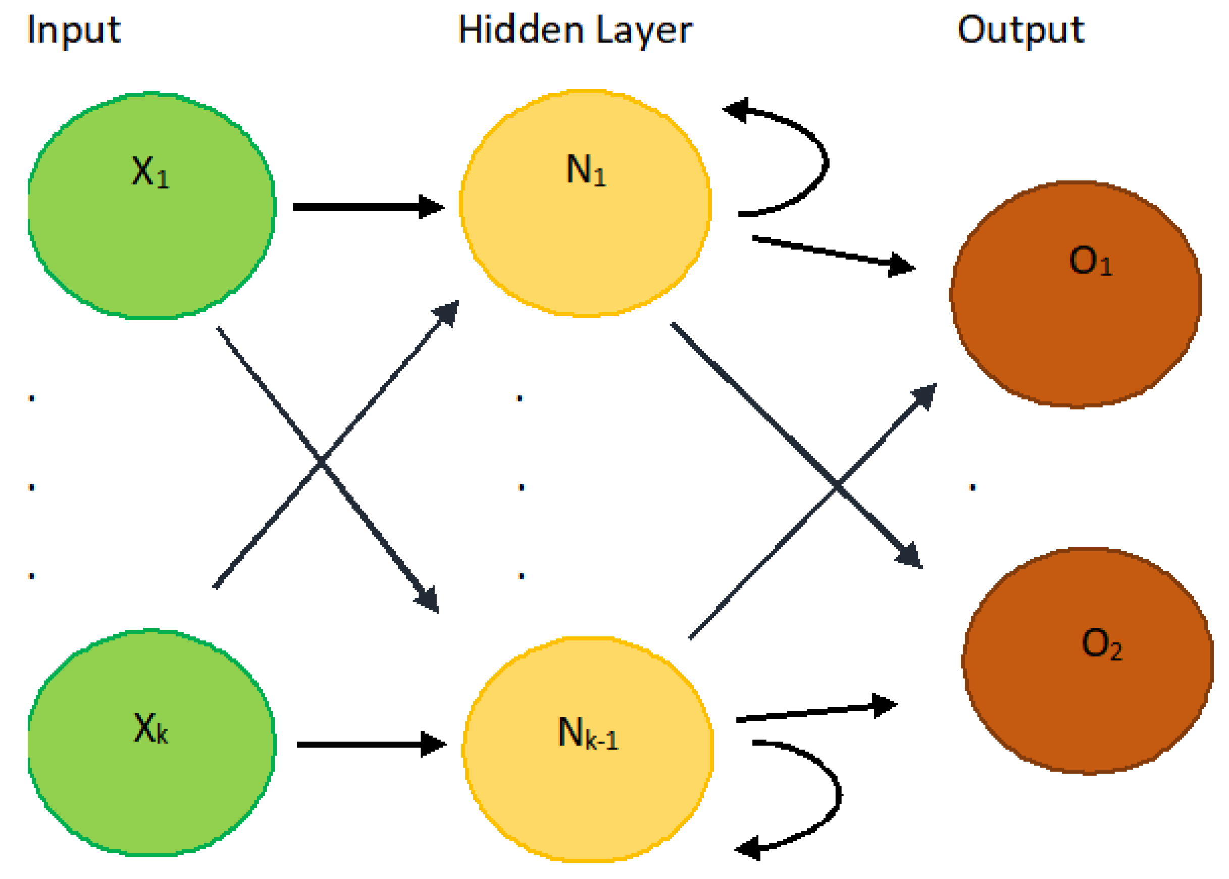
3.1. Univariate Machine Learning Methods

Autoregressive integrated moving average (ARIMA) and exponential smoothing models are the most widely used forecasting time-series models for analyzing univariate time-series data. ARIMA models aim to describe the autocorrelations in the data, while exponential smoothing models are based on a description of the trend and seasonality in the data (Hyndman and Athanasopoulos 2021). Holt’s exponential smoothing model is a popular smoothing model for forecasting data with trends. Swamidass (2000) explained that Holt’s model has three separate equations that work together to generate a final forecast: The first is a basic smoothing equation that directly adjusts the last smoothed value for last period’s trend. The trend itself is updated over time through the second equation, where the trend is expressed as the difference between the last two smoothed values. Finally, the third equation is used to generate the final forecast. Holt’s model uses two parameters: one for the overall smoothing, and the other for the trend smoothing equation. The method is also called double exponential smoothing or trend-enhanced exponential smoothing. Since exponential smoothing models can capture a variety of trends and seasonal forecasting patterns (such as additive or multiplicative), and combinations of the two, Petropoulos and Makridakis (2020) forecast confirmed cases of COVID-19 by using the exponential smoothing family, which has shown good forecast accuracy over several forecasting competitions, and is especially suitable for short series. Holt’s exponential smoothing, as shown by Hyndman and Athanasopoulos (2021), fits a time-series model using smoothing level and smoothing slope. Furthermore, we used a Python package known as Forecast_x, which provides different naïve models (Naive, Seas Naive, Mean Two Periods, Mean Three Periods, Half Seas Mean, Seas Period Mean, Double Seas Mean, Seas Growth, Expo Weighted, Threefith Mean, Multi Seas Mean, Seas Double Mean Growth, Grand Mean, Smooth Grand Mean, Last Seas Mean, Current Mean Seas, Smooth Double Seas Naive, Truncated Mean, Harmonic Mean, Heronian Mean) for fitting multiple time series due to its powerful flexibility and easy usage.

The conventional univariate time-series model known as ARIMA was employed to compare the univariate and multivariate machine learning time-series models. We used the Auto ARIMA package in Python for the data analysis. Each of the cryptocurrency datasets were split into different training (70%, 80%, and 90%) and test sets so that the accuracy of the model could be measured.

The univariate machine learning models known as DLN, RNN, and LSTM create a function that makes their respective models and future predictions. We proceed to normalize and reshape the training sets (70%, 80%, and 90%) into a 3D array with five time stamps and one feature at each step. The test set was also rescaled and used to make predictions on it. Figure 4 and Figure 5 show the outline of DNN, RNN, and LSTM.

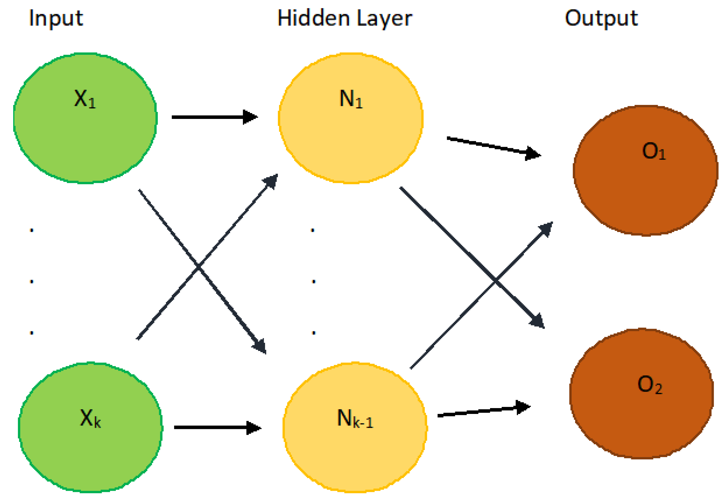
3.2. Multivariate Machine Learning Method

We employed a multivariate LSTM machine learning model for forecasting the price log returns of all of the cryptocurrencies. The idea for this paper came from the computational problem of vector autoregressive (VAR) models with many covariate time-series variables. The VAR is a classical multivariate forecasting time-series model, but faces difficulties in computing the covariance matrix with many covariate time-series variables (usually more than five time-series covariates). Therefore, we considered an alternative multivariate time-series model by using a multivariate LSTM machine learning model. Before applying the multivariate LSTM method to the data, we scaled the data by using two functions: MinMaxScaler(feature_range=(−1, 1))—a scaler between −1 and 1—and scaler.fit_transform(values), a Python package that transforms the values. Afterwards, a ‘for’ loop was created based on three training sets (70%, 80%, and 90% of the data). In this ‘for’ loop, the model was created based on the training and testing sets, and was then used to predict each of the cryptocurrencies for both the training and testing sets. The testing, training, and prediction sets were then renormalized. The outline of the LSTM multivariate machine learning model for price log returns of each cryptocurrency is:

BTC(t) = BTC(t − 1) + ETH(t − 1) + USDT(t − 1) + XRP(t − 1) + BNB(t − 1) + ADA(t − 1) + FLOW(t − 1) + USDC(t − 1) + DOGE(t − 1) + UNI(t − 1) + ε(t)
ETH(t) = BTC(t − 1) + ETH(t − 1) + USDT(t − 1) + XRP(t − 1) + BNB(t − 1) + ADA(t − 1) + FLOW(t − 1) + USDC(t − 1) + DOGE(t − 1) + UNI(t − 1) + ε(t)
USDT(t) = BTC(t − 1) + ETH(t − 1) + USDT(t − 1) + XRP(t − 1) + BNB(t − 1) + ADA(t − 1) + FLOW(t − 1) + USDC(t − 1) + DOGE(t − 1) + UNI(t − 1) + ε(t)
XRP(t) = BTC(t − 1) + ETH(t − 1) + USDT(t − 1) + XRP(t − 1) + BNB(t − 1) + ADA(t − 1) + FLOW(t − 1) + USDC(t − 1) + DOGE(t − 1) + UNI(t − 1) + ε(t)
BNB(t) = BTC(t − 1) + ETH(t − 1) + USDT(t − 1) + XRP(t − 1) + BNB(t − 1) + ADA(t − 1) + FLOW(t − 1) + USDC(t − 1) + DOGE(t − 1) + UNI(t − 1) + ε(t)
ADA(t) = BTC(t − 1) + ETH(t − 1) + USDT(t − 1) + XRP(t − 1) + BNB(t − 1) + ADA(t − 1) + FLOW(t − 1) + USDC(t − 1) + DOGE(t − 1) + UNI(t − 1) + ε(t)
FLOW(t) = BTC(t − 1) + ETH(t − 1) + USDT(t − 1) + XRP(t − 1) + BNB(t − 1) + ADA(t − 1) + FLOW(t − 1) + USDC(t − 1) + DOGE(t − 1) + UNI(t − 1) + ε(t)
USDC(t) = BTC(t − 1) + ETH(t − 1) + USDT(t − 1) + XRP(t − 1) + BNB(t − 1) + ADA(t − 1) + FLOW(t − 1) + USDC(t − 1) + DOGE(t − 1) + UNI(t − 1) + ε(t)
DOGE(t) = BTC(t − 1) + ETH(t − 1) + USDT(t − 1) + XRP(t − 1) + BNB(t − 1) + ADA(t − 1) + FLOW(t − 1) + USDC(t − 1) + DOGE(t − 1) + UNI(t − 1) + ε(t)
UNI(t) = BTC(t − 1) + ETH(t − 1) + USDT(t − 1) + XRP(t − 1) + BNB(t − 1) + ADA(t − 1) + FLOW(t − 1) + USDC(t − 1) + DOGE(t − 1) + UNI(t − 1) + ε(t)

(1)

where ε(t) is error term of time point t, and we set the multivariate LSTM with 128 epochs by using the function model.add(LSTM(128, input_shape = (10, 10))).

3.3. Forecast Evaluation

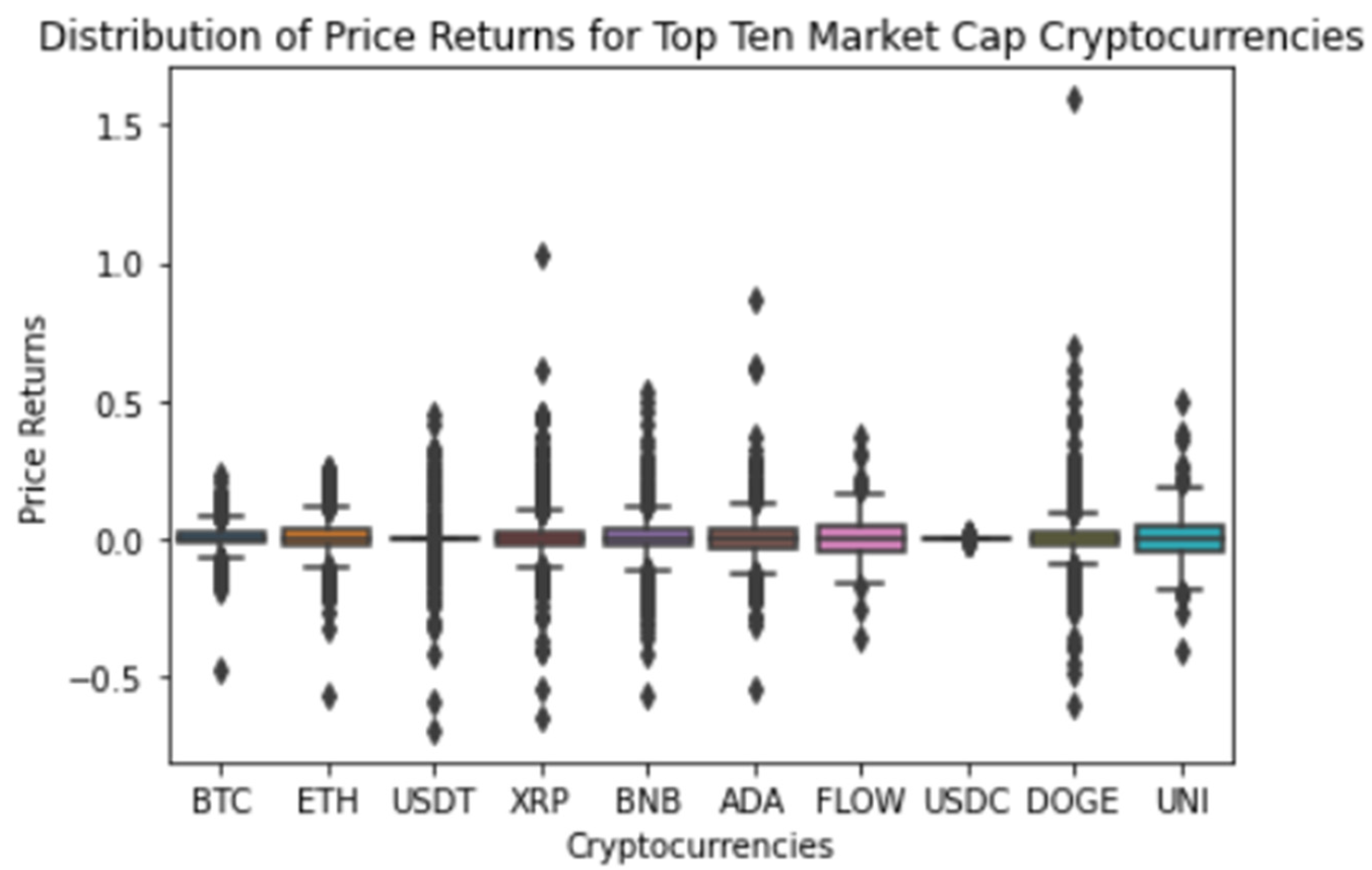
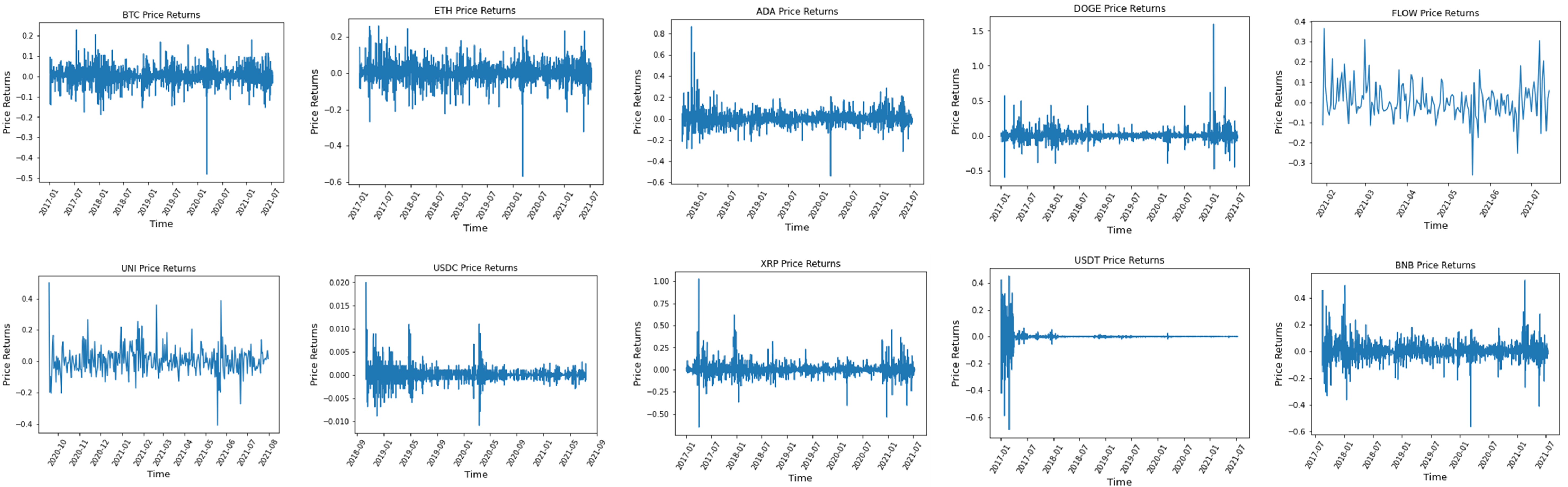
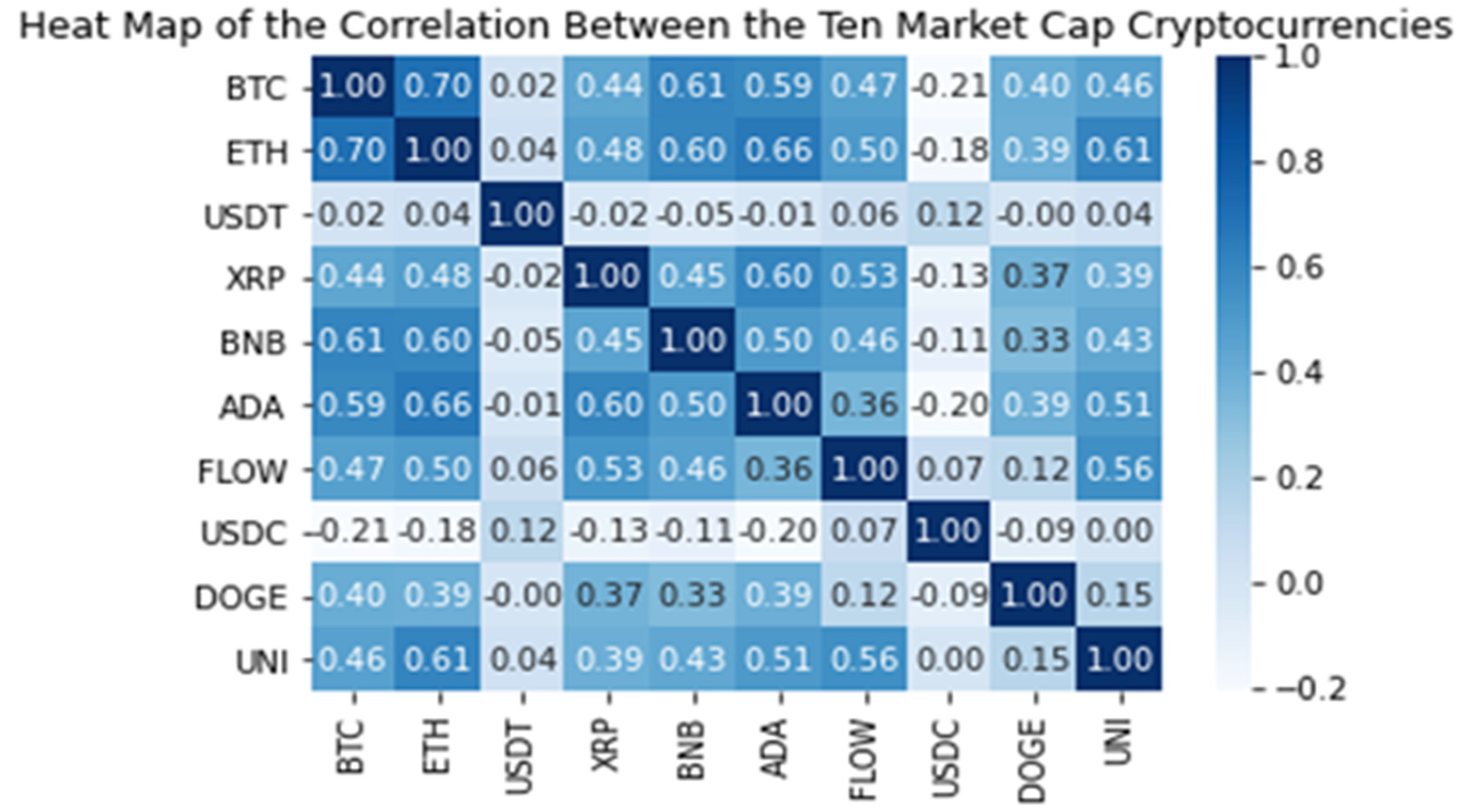
For this subsection, we measured the predictive accuracy of our machine learning models. The models used three different training sets (70%, 80%, and 90% of each cryptocurrency’s data). We compared the predicted values and actual values ($y_t \mathrm{and} {\widehat{y}}_t$). where t = 1, 2, …, n. (n = the total number of test dataset). We employed two measures for predictive accuracy:

Root-mean-square (prediction) error (RMSE):

$$RMSE=\sqrt{\frac{{{\displaystyle \sum }}_{t=1}^n{\left(y_t-{\widehat{y}}_t\right)}^2}{n}}$$

(2)

and the mean absolute error deviation (MAD):

$$MAD=\frac{{{\displaystyle \sum }}_{t=1}^n\left|y_t-{\widehat{y}}_t\right|}{n}.$$

(3)

The error metrics such as the MAD and RMSE were used to analyze the performance of the methods. Mean absolute error is not sensitive to outliers, as they are weighted less than the other observations when comparing actual and predicted values. Root-mean-square error takes bias and variance into account, but normalizes the units. Each method also produces plots based on the actual and predicted price returns for visualization purposes.

4. Data Analysis

Low results for the metric measures can be interpreted as the model being a good fit for the data, and the future price log returns are accurate to a point. When looking at the prediction error measures such as RMSE in

Table 2. Measuring predictions using RMSE.

70%	RMSE
	DNN	RNN	LSTM	ARIMA	FORECASTX	HOLTS	Multivariate LSTM
BTC	0.120	0.107	0.045	0.049	0.046	0.046	0.046
ETH	0.153	0.080	0.087	0.066	0.061	0.061	0.055
XRP	0.003	0.011	0.012	0.002	0.002	0.003	0.001
USDT	0.146	0.140	0.092	0.086	0.079	0.080	0.068
BNB	0.079	0.100	0.069	0.075	0.069	0.070	0.060
ADA	0.094	0.125	0.215	0.074	0.068	0.068	0.053
DOGE	0.167	0.185	0.001	0.001	0.093	0.090	0.093
USDC	0.008	0.045	0.122	0.132	0.001	0.001	0.001
FLOW	0.347	0.127	0.095	0.097	0.120	0.119	0.103
UNI	0.381	0.111	0.104	0.104	0.095	0.096	0.072
80%	RMSE
	DNN	RNN	LSTM	ARIMA	FORECASTX	HOLTS	Multivariate LSTM
BTC	0.042	0.067	0.041	0.045	0.042	0.043	0.044
ETH	0.085	0.084	0.088	0.065	0.059	0.059	0.064
XRP	0.001	0.005	0.008	0.001	0.001	0.001	0.001
USDT	0.164	0.143	0.116	0.099	0.090	0.090	0.080
BNB	0.087	0.083	0.079	0.086	0.079	0.079	0.070
ADA	0.086	0.142	0.212	0.081	0.074	0.073	0.061
DOGE	0.123	0.148	0.001	0.001	0.107	0.102	0.117
USDC	0.008	0.050	0.146	0.154	0.001	0.001	0.001
FLOW	0.566	0.194	0.107	0.110	0.139	0.139	0.124
UNI	0.387	0.212	0.111	0.118	0.107	0.107	0.081
90%	RMSE
	DNN	RNN	LSTM	ARIMA	FORECASTX	HOLTS	Multivariate LSTM
BTC	0.070	0.077	0.047	0.050	0.046	0.048	0.031
ETH	0.117	0.083	0.075	0.069	0.063	0.063	0.056
XRP	0.001	0.010	0.010	0.001	0.001	0.001	0.001
USDT	0.250	0.143	0.130	0.109	0.098	0.102	0.030
BNB	0.196	0.080	0.081	0.093	0.122	0.092	0.046
ADA	0.092	0.259	0.165	0.081	0.072	0.072	0.034
DOGE	0.119	0.119	0.001	0.001	0.117	0.111	0.050
USDC	0.004	0.052	0.136	0.159	0.001	0.001	0.001
FLOW	0.242	0.136	0.120	0.117	0.138	0.231	0.130
UNI	0.097	0.107	0.441	0.082	0.077	0.074	0.055

and MAD in

Table 3. Measuring predictions using MAD.

70%	MAD
	DNN	RNN	LSTM	ARIMA	FORECASTX	HOLTS	Multivariate LSTM
BTC	0.061	0.063	0.029	0.031	0.029	0.030	0.036
ETH	0.096	0.071	0.056	0.042	0.041	0.041	0.045
XRP	0.066	0.065	0.056	0.050	0.047	0.049	0.048
USDT	0.001	0.008	0.006	0.001	0.001	0.003	0.001
BNB	0.045	0.044	0.043	0.047	0.043	0.045	0.044
ADA	0.055	0.106	0.161	0.053	0.048	0.049	0.039
DOGE	0.143	0.125	0.064	0.062	0.056	0.058	0.055
USDC	0.005	0.030	0.001	0.001	0.000	0.006	0.001
FLOW	0.106	0.121	0.079	0.081	0.067	0.065	0.076
UNI	0.270	0.134	0.067	0.066	0.066	0.066	0.059
80%	MAD
	DNN	RNN	LSTM	ARIMA	FORECASTX	HOLTS	Multivariate LSTM
BTC	0.388	0.056	0.030	0.034	0.030	0.031	0.034
ETH	0.063	0.068	0.066	0.046	0.043	0.043	0.049
XRP	0.086	0.122	0.073	0.061	0.056	0.057	0.055
USDT	0.001	0.009	0.004	0.001	0.001	0.001	0.001
BNB	0.053	0.064	0.051	0.055	0.050	0.051	0.047
ADA	0.064	0.124	0.146	0.059	0.053	0.053	0.043
DOGE	0.137	0.070	0.072	0.077	0.067	0.067	0.069
USDC	0.005	0.054	0.001	0.001	0.001	0.001	0.001
FLOW	0.091	0.108	0.077	0.089	0.079	0.073	0.094
UNI	0.400	0.110	0.076	0.052	0.076	0.075	0.062
90%	MAD
	DNN	RNN	LSTM	ARIMA	FORECASTX	HOLTS	Multivariate LSTM
BTC	0.039	0.068	0.034	0.036	0.034	0.036	0.028
ETH	0.067	0.059	0.056	0.048	0.047	0.048	0.044
XRP	0.096	0.098	0.090	0.064	0.066	0.071	0.028
USDT	0.002	0.005	0.005	0.001	0.001	0.001	0.001
BNB	0.136	0.081	0.058	0.056	0.100	0.069	0.038
ADA	0.075	0.075	0.098	0.051	0.052	0.053	0.029
DOGE	0.125	0.097	0.090	0.081	0.089	0.203	0.046
USDC	0.008	0.057	0.001	0.001	0.001	0.001	0.001
FLOW	0.093	0.107	0.091	0.071	0.089	0.080	0.109
UNI	0.096	0.128	0.543	0.039	0.059	0.058	0.050

, the multivariate LSTM time-series model seems to have consistently lower numbers for the price log returns of cryptocurrencies compared to the univariate machine learning methods, except for the case of BTC, because BTC is a major cryptocurrency that influences the prices of all other Altcoins. For the prediction for the log returns of BTC, a univariate LSTM time-series model can be a good prediction model. With the log returns of nine Altcoins, we can conclude that the multivariate machine learning method has a better fit and forecast ability compared to the univariate machine learning methods.

After analyzing the results from the visualizations and metric measure tables on the prediction accuracy of the univariate and multivariate machine learning methods for the price returns of cryptocurrencies, it should be noted that the performance of the univariate machine learning methods changed greatly for the different training sets compared to the multivariate machine learning method. In order to compare predictive accuracy across models, the differences in forecasting abilities across models can be tested as described by Diebold and Mariano (1995).

5. Conclusions

We compared the univariate machine learning time-series methods with the multivariate LSTM machine learning method in terms of prediction measure errors. The classical time series VAR model cannot handle many covariate time-series data because of the difficulty of computing the covariance matrix. However, we proved from this research that the multivariate LSTM machine learning method can handle covariate time-series data for 10 cryptocurrencies without experiencing computational difficulties. We concluded that the multivariate LSTM machine learning method generated better performance compared to the univariate machine learning time-series methods in terms of the prediction measures errors for the top 10 cryptocurrencies. Our future research question is whether the performance of the multivariate machine learning method known as long short-term memory networks is dependent on more vast amounts of data—such as dates and cryptocurrencies—than were used in this study. There is also a possibility that the machine learning methods known as GARCH or multivariate GARCH may produce better results, because they may be able to account for the high volatility in cryptocurrencies. By using univariate and multivariate machine learning methods to predict the price log returns of cryptocurrencies based on their previous values and relationships with one another, a better understanding can be reached as to whether they can be used to predict things such as the stock market, cryptocurrency market, and weather. Improvements can also be made to the univariate and multivariate machine learning models used in this study by adjusting the parameters of the models.

References

1. Akyildirim, Erdinc, Ahmet Goncu, and Ahmet Sensoy. 2021. Prediction of cryptocurrency returns using machine learning. Annals of Operations Research 297: 3–36. [Google Scholar] [CrossRef]
2. Diebold, F. X., and R. S. Mariano. 1995. Comparing Predictive Accuracy. Journal of Business and Economic Statistics 13: 253–63. [Google Scholar]
3. Hyndman, Rob J., and George Athanasopoulos. 2021. Forecasting: Principles and Practice, 3rd ed. Melbourne: OTexts. [Google Scholar]
4. Hyun, Steve, Jimin Lee, Jong-Min Kim, and Chulhee Jun. 2019. What Coins lead in the Cryptocurrency Market? Using Copula and Neural Networks Model. Journal of Risk and Financial Management 12: 132. [Google Scholar] [CrossRef] [Green Version]
5. Katsiampa, Paraskevi. 2017. Volatility estimation for Bitcoin: A comparison of GARCH models. Economics Letters 158: 3–6. [Google Scholar] [CrossRef] [Green Version]
6. Katsiampa, Paraskevi. 2019. An empirical investigation of volatility dynamics in the cryptocurrency market. Research in International Business and Finance 50: 322–35. [Google Scholar] [CrossRef]
7. Kim, Jong Min, Chulhee Jun, and Junyoup Lee. 2021. Forecasting the volatility of the cryptocurrency market using GARCH and Stochastic Volatility. Mathematics 9: 1614. [Google Scholar] [CrossRef]
8. Kim, Jong Min, Seong-Tae Kim, and Sangjin Kim. 2020. On the Relationship of Cryptocurrency Price with US Stock and Gold Price using Copula Models. Mathematics 8: 1859. [Google Scholar] [CrossRef]
9. Mostafa, Fahad, Pritam Saha, Mohammad R. Islam, and Nguyet Nguyen. 2021. GJR-GARCH Volatility Modeling under NIG and ANN for Predicting Top Cryptocurrencies. Journal of Risk and Financial Management 14: 421. [Google Scholar] [CrossRef]
10. Nakamoto, Satoshi. 2008. Bitcoin: A Peer-to-Peer Electronic Cash System. Available online: https://bitcoin.org/bitcoin.pdf (accessed on 1 September 2021).
11. Petropoulos, Fotios, and Spyros Makridakis. 2020. Forecasting the novel coronavirus COVID-19. PLoS ONE 15: e0231236. [Google Scholar] [CrossRef] [PubMed]
12. Phillip, Andrew, Jennifer Chan, and Shelton Peiris. 2019. On long memory effects in the volatility measure of Cryptocurrencies. Finance Research Letters 28: 95–100. [Google Scholar] [CrossRef]
13. Plakandaras, Vasilios, Elie Bouri, and Rangan Gupta. 2021. Forecasting bitcoin returns: Is there a role for the US–China trade war? Journal of Risk 23: 3. [Google Scholar]
14. Shahzad, Syed Jawad Hussain, Elie Bouri, Mobeen Ur Rehman, and David Roubaud. 2021. The Hedge Asset for Brics Stock Markets: Bitcoin, Gold, or Vix. Kiel: The World Economy. [Google Scholar]
15. Swamidass, Paul M. 2000. Holt’s Forecasting Model. In Encyclopedia of Production and Manufacturing Management. Boston: Springer. [Google Scholar]
16. Wang, Pengfei, Wei Zhang, Xiao Li, and Dehua Shen. 2019. Is cryptocurrency a hedge or a safe haven for international indices? A comprehensive and dynamic perspective. Finance Research Letters 31: 1–18. [Google Scholar] [CrossRef]
Figure 1. Boxplot of 10 cryptocurrencies based on market cap.
Jrfm 14 00486 g001
Figure 2. Time-series plot of price log returns of 10 cryptocurrencies.
Jrfm 14 00486 g002
Figure 3. Correlation plot of price returns of 10 cryptocurrencies based on market cap.
Jrfm 14 00486 g003
Figure 4. Deep learning neural network (DNN) outline.
Jrfm 14 00486 g004
Figure 5. RNN and LSTM outline.
Jrfm 14 00486 g005