For Professional Investors only. All investments involve risk, including the possible loss of capital.
These materials represent the views and opinions of the authors regarding the economic conditions, asset classes, or financial instruments referenced herein and are not necessarily the views of PGIM Quantitative Solutions.
PGIM Quantitative Solutions -20200219-102.
1. Introduction
Value portfolios have delivered lackluster results over the last decade. Most asset classes have been affected. Our results show that, on average, a diversified multi-asset value portfolio in developed markets generated about 0.60% annualized return per unit of risk from 1990–2009. In contrast, the return of the same portfolio since 2010 was negative. Investors have not been compensated for their exposure to value for a full decade.
Recent performance difficulties within value have left many investors wondering how to make sense of these results. The debate centers around several conflicting explanations:
2. Natural variation in bottom-up fundamentals and factor performance unrelated to business cycles (
Singh et al. 2019).
We contribute to the literature by focusing on the interaction of the value factor payoff with the macroeconomic environment, while acknowledging other possible explanations.
Ilmanen et al. (
2019) report that multi-asset value factor returns tend to be higher when the economy is slowing down. However, after further robustness checks, they subsequently argue that there is actually not a reliable relationship between value and macroeconomic risk. On the other hand,
Bellone et al. (
2019) studied the performance of multi-asset portfolios during different market regimes and found that a multi-asset value portfolio outperforms during the cyclical recovery of equity markets and in periods of rising interest rates. They also found significant differences in value portfolio behavior across asset classes. According to their research, bond and equity value portfolios exhibit a strong cyclical bias, and currency value portfolios display both moderate defensive and cyclical biases.
Recent value underperformance has called into question whether the value payoff is cyclically low, or if there are more structural challenges ahead. To shed new light on this debate, we borrow the framework introduced by
Aiolfi and Tokat-Acikel (
2019) and use holdings-based and factor-mimicking portfolio analyses to identify the typical macroeconomic characteristics of multi-asset value portfolios. We provide insights into the relationship between value factors and macro fundamentals, how value evolves over a typical business cycle, and if this changed in the last decade versus historical time periods.
Our approach leads to several significant empirical contributions. First, we explore whether or not the value factor payoff is cyclical, using forward-looking consensus growth expectations. Our analysis suggests that the value payoff is very weakly related to a global business cycle. This result is similar to
Ilmanen et al. (
2019) and
Yara et al. (
2019).
Next, taking advantage of the cross-country inflation and growth expectations implicit in every value portfolio we studied, we derive a time series of the value portfolios’ macro characteristics that we can then use to estimate average characteristics over different time periods. We establish that growth and inflation exposures vary over time, but that they have been, on average, positive over the full history back to 1990. This differs notably from the stock selection literature that shows growth stock portfolios to be expensive (
Fama and French 1992). In addition, we also find that the value payoff was higher, on average, when the net relative macro exposures were also higher.
Using an alternate approach of factor-mimicking portfolio performance attribution methodology, we find further evidence that the payoff to value portfolios in various asset classes is strongly linked to relative growth and inflation expectations across countries. Our results provide fresh evidence of a link between the well-known macroeconomic exposures of traditional asset classes and those of multi-asset risk premia portfolios (
Aiolfi and Tokat-Acikel 2019).
Lastly, we shed new light on the underperformance of the value payoff since the GFC. Our results show that a diversified multi-asset value portfolio bought assets of countries with both relatively higher inflation and growth before 2010. However, this characteristic has changed over the last decade. We find that cheaper assets have had much lower net relative macro exposures post 2009, compared to earlier time periods. This suggests that weakness in the recent value payoff is due to normal factor return variability and weaker net growth exposure during the cyclical economic recovery from the GFC of 2008.
The remainder of the paper is organized as follows.
Section 1 defines and reviews value strategies across asset classes.
Section 2 describes our dataset and the portfolio construction method.
Section 3 replicates stylized value results.
Section 4 explores whether or not the value payoff is cyclical.
Section 5 explores growth and inflation exposures of value factor portfolios using our new methodology.
Section 6 explores what has changed in value exposures since the 2008 GFC.
Section 7 provides our conclusions.
2. Value Strategies across Asset Classes
The underlying goal in value investing is determining whether an asset’s price is cheap or expensive relative to its intrinsic value. While prices may deviate from fundamentals due to investor over- or underreaction, or changes in the discount rate, they should ultimately revert to intrinsic value over the long run.
The most popular application of value is found in equity markets. The equity value trade involves buying high fundamental value-to-price (cheap) equities, while selling low fundamental value-to-price (expensive) ones. There is a long-standing debate in academia about why an investor seeking value exposure is compensated.
1 Fama and French (
1992) argue that value stocks are risky, and that higher book/price may be a proxy for relative distress factors, so the value premium compensates for additional risk taken on in the portfolio.
Lakonishok et al. (
1994) attribute the value premium to the tendency of investors to extrapolate earnings growth too far into the future. Such investors avoid buying stocks that have done poorly in the recent past, the argument goes, so the value premium is due to behaviorally-induced mispricing. Most other academic research on the equity value premium fall into one of these two camps: compensation for risk versus behavior (pricing mistakes). We believe that both systematic economic risk and behavioral biases contribute to the value premium.
Determining the intrinsic value of an equity may be a difficult task. Discounted cash flow (DCF) models attempt to forecast future equity cash flows using estimates of growth, payout ratios, and discount rates. These, however, are subject to very strong assumptions. Even small changes in underlying assumptions can lead to large deviations in value estimates.
2 Instead, simple proxies such as book/price have been shown to be effective tools in measuring value (
Asness et al. 2013). While in stock selection literature (e.g.,
Fama and French 1992), expensive stocks based on book/price multiples are considered growth stocks, we show in the following sections that this terminology is not accurate for country equities.
Fixed income valuation appears to be a more straightforward task than equity valuation. While cash flows, absent defaults, are well determined, the discount rate is not. The discount rate depends on estimates of future inflation, changes in time preferences, perceived changes in default risks, and other factors. The most discounted (cheapest) bond would simply be the bond with the highest yield-to-maturity (YTM). However, in practice, a selection solely based on YTM would likely lead to investing in bonds issued by sovereigns with higher inflation expectations and/or higher probability of default. Therefore, we have to consider economic fundamentals when deciding whether a government bond is cheap or expensive. Value strategies in fixed income are constructed by ranking countries by their real yield (
Asness et al. 2013).
Finally, one of the oldest and most popular
3 measures of currency fair value is the purchasing power parity (PPP) implied exchange rate. The concept is based on the law of one price. It states that in the absence of transaction costs and official trade barriers, identical goods will have the same price in different markets when prices are expressed in the same currency. Suppose that the prices of foreign goods are unusually high relative to the prices of domestic goods. To obtain this ratio back to a more “normal” level, either foreign prices need to decline, or domestic prices need to rise, or both. In practice, the prices of local goods tend to be sticky, whereas the exchange rate is highly flexible. The adjustment to the PPP exchange rate occurs through trade flows. Absenting trade barriers, demand would flow from the country with the higher prices to the country with cheaper goods, weakening the currency of the country with higher-priced goods. Over a sufficiently long period, countries with high (low) inflation relative to their trading partners tend to experience currency depreciation (appreciation). The tendency for PPP to hold over the long run leads immediately to a value-oriented investment strategy predicated on mean reversion: buy undervalued currencies and sell overvalued currencies.
While rigorous economic studies (see
Abuaf and Jorion 1990;
Flood and Taylor 1996;
Imbs et al. 2005) have documented a statistically significant tendency for exchange rates to revert to their PPP-implied values over time, a variety of forces, including monetary and fiscal policies, can create countervailing pressures that prevent currencies from reverting to their intrinsic value in the intermediate term. The risk that these discrepancies will continue or deepen before reverting to fair value provides the value premium that can be exploited.
3. Data Collection and Portfolio Construction
This section describes the return sources, value measures, and approach to portfolio construction used in our empirical analysis.
3.1. Investment Universe and Data Sources
In our empirical analysis, we sought to use only liquid, investable assets that a global macro investor could trade. Our data extends back to 1990, since most of the assets in our study were uninvestable before 1990 due to regulatory or liquidity restraints. Our analysis does not include commodities, for two reasons. First, it is difficult to define an intrinsic value for commodities on which to anchor prices. Second, commodities are global assets, and therefore do not naturally map into the economic characteristics of individual countries. We also exclude analysis of single stock-based value factors, as our macroeconomic exposure-based approach does not naturally apply to single stocks.
Currencies: We focused on the most liquid currencies traded by active currency investors. The developed market currency portfolio consists of the Australian dollar, Canadian dollar, euro, Japanese yen, Norwegian krone, Swedish krona, New Zealand dollar, British pound sterling, and Swiss franc. For the time period prior to 1999, we excluded legacy euro currencies, and approximated the euro with the Deutsche mark. We obtained spot and forward exchange rates from WMR, Bloomberg, and various brokers. We computed returns for one-month currency forwards from the perspective of a US-based investor and approximated returns using spot exchange rates and the one-month LIBOR/deposit rate.
Country Equities: We used the local returns of MSCI
4 country indices in the following 11 developed countries: US, UK, Canada, Australia, Japan, France, Germany, Italy, Spain, Sweden, and Switzerland. Returns and dividend yields were sourced from MSCI.
Bonds: We used 10-year bond futures indices hedged to USD from Bloomberg for the following countries: US, UK, Canada, Australia, Japan, and Germany. For time periods prior to the introduction of the Bloomberg futures indices, we backfilled the returns with synthetic bond futures returns similar to
Koijen et al. (
2018). We sourced 10- and two-year yields on the bonds from Bloomberg.
3.2. Value Measures
We closely followed the existing literature in each asset class for our value measures. The purpose of this paper is to shed light on macroeconomic characteristics of value, so we did not focus on how to improve the factor measurement.
Currencies: We measured value using the idea of purchasing power parity (PPP). To be more specific, it is the currency’s spot exchange rate deviation from OECD PPP-based fair value. Currencies with higher deviation from their fair value based on OECD PPP are considered more expensive.
Country Equities: We used the 12-month trailing earnings to price (E/P) from MSCI country indices to measure value for country equities. The country equity with higher E/P is cheaper.
Bonds: We measured bond value as the real yield, the difference between 10-year yield and constant one-year inflation forecasts using forecasts from Consensus Economics. Bonds with higher real yields are cheaper.
3.3. Macroeconomic Measures
We built real GDP and inflation constant one-year forecasts from Consensus Economics to approximate real growth and inflation expectations for the set of countries of interest. Consensus Economics surveys over 250 prominent financial and economic forecasters for their estimates of a range of variables, including future growth and inflation. More than 20 countries are covered, with data going back to 1990. One advantage of using forecasts instead of realized macroeconomic data is that such forecasts are not revised and are not subject to forward-looking biases. Participants provide current and next-year forecasts for measures of interest, typically released in the middle of the month. Incoming survey responses are then processed and checked for accuracy, completeness, and integrity, and aggregated into a consensus average. We created constant one-year forecasts by time-weighting the forward year-one and year-two forecasts for inflation
and real GDP growth (
in each country of interest. The forecasted nominal GDP growth (
is the sum of inflation and real GDP growth constant one-year expectations. We also created global inflation
and real GDP growth (
) by aggregating country-specific forecasts using GDP weights.
5,6 3.4. Portfolio Construction
We built portfolios of assets to implement our strategies in line with current industry and research practices. At the end of each month, we sorted the assets according to the value measure specific to each asset class (as described in the previous section) and formed zero-cost long–short portfolios, taking long positions in the undervalued (cheap) assets and shorting the overvalued (expensive) ones. We rebalanced the portfolios on a monthly basis over the sample time frame, from January 1990–February 2021, ignoring transaction costs.
Following
Asness et al. (
2013) for any security
in asset class
at time
t with value measure
we weighted securities in a linear fashion according to the following scheme:
The weights across all securities sum to zero, representing a dollar-neutral long–short portfolio where
is an asset class-specific scalar, such that the ex-post annualized volatility of each portfolio is comparable and equal to 5% over the entire sample period.
Table 1 shows an example for constructing a long–short value portfolio of fixed income assets using real yield as the value measurement. The real yield for each bond is calculated by using nominal yield and Consensus Economics inflation forecast data as of the end of February of 2021. The assets are ranked based on their factor values: the cheaper the asset, the higher the rank. The factor weights are multiplied by a scalar to obtain 5% ex-post annualized volatility.
We also built a reference-diversified multi-asset value portfolio by taking an equal volatility-weighted average of the three individual value portfolios (developed country equities, developed currencies, and developed bonds). We then rescaled the resulting combined portfolio to 5% ex-post annualized volatility. This procedure is similar to that used by
Asness et al. (
2013) and
Koijen et al. (
2018).
4. Stylized Empirical Results
Table 2 shows the historical performance statistics for the diversified multi-asset value portfolio, as well as the asset class-specific value portfolios from 1990 through February 2021. Broadly speaking, all value strategies generated positive excess returns, but with a large dispersion in information ratios, ranging from 0.11 in government bonds to 0.39 in currencies. The diversified multi-asset value portfolio has an information ratio of 0.35, confirming the significant diversification benefits of applying value trades across asset classes, as found in
Asness et al. (
2013,
2015),
Baz et al. (
2015),
Baltussen et al. (
2019), and
Ilmanen et al. (
2019).
Table 2 also shows that the multi-asset value portfolio has negative skewness, is weakly positively correlated to global equities, and is slightly negatively correlated to global bonds. While our value factor portfolios are constructed from a USD investor perspective, we find only a small correlation (0.17) with the US dollar index (DXY). These properties are less consistent when observing asset class-specific value portfolios.
Performance statistics are reported for value strategies in developed currencies (currency), developed country equities (equity), developed country bonds (fixed income), and developed diversified multi-asset portfolios (multi-asset value). Statistics are computed from a monthly return series over the sample time period: January 1990–February 2021. For developed country bonds, the sample time period is January 1991–February 2021. Portfolios are rebalanced monthly. Weights are scaled so that the ex-post volatility of each strategy is set to 5% over the entire backtest period for comparison purposes. Reported returns do not include transaction costs.
We find that the performance of value in government bonds, currencies, and country equities is positively correlated with global equity returns, while the correlation with global bond returns and the US dollar index are more mixed. It is particularly interesting to notice that value in currencies displays positive correlation to both global equities and the US dollar. This suggests a subtler cycle of performance with a both a moderate cyclical and defensive bias, as suggested by
Bellone et al. (
2019). This indicates that style dynamics at the asset class level are not only influenced by business cycle dynamics, but also by more idiosyncratic sources of risk.
Table 3 supports these findings and shows that the correlations of value portfolios across various asset classes are close to zero when measured at monthly frequency. The implication argues for a small systematic component across value portfolios in different asset classes, even though these portfolios share the same theoretical foundations and are applied to an overlapping set of developed countries.
Average correlations are reported among carry strategies in developed currencies (currency), developed country equities (equity), and developed country bonds (fixed income). Statistics are computed from monthly return series over the sample time period: January 1990–February 2021. For developed country bonds, the sample time period is January 1991–February 2021. Portfolios are rebalanced monthly.
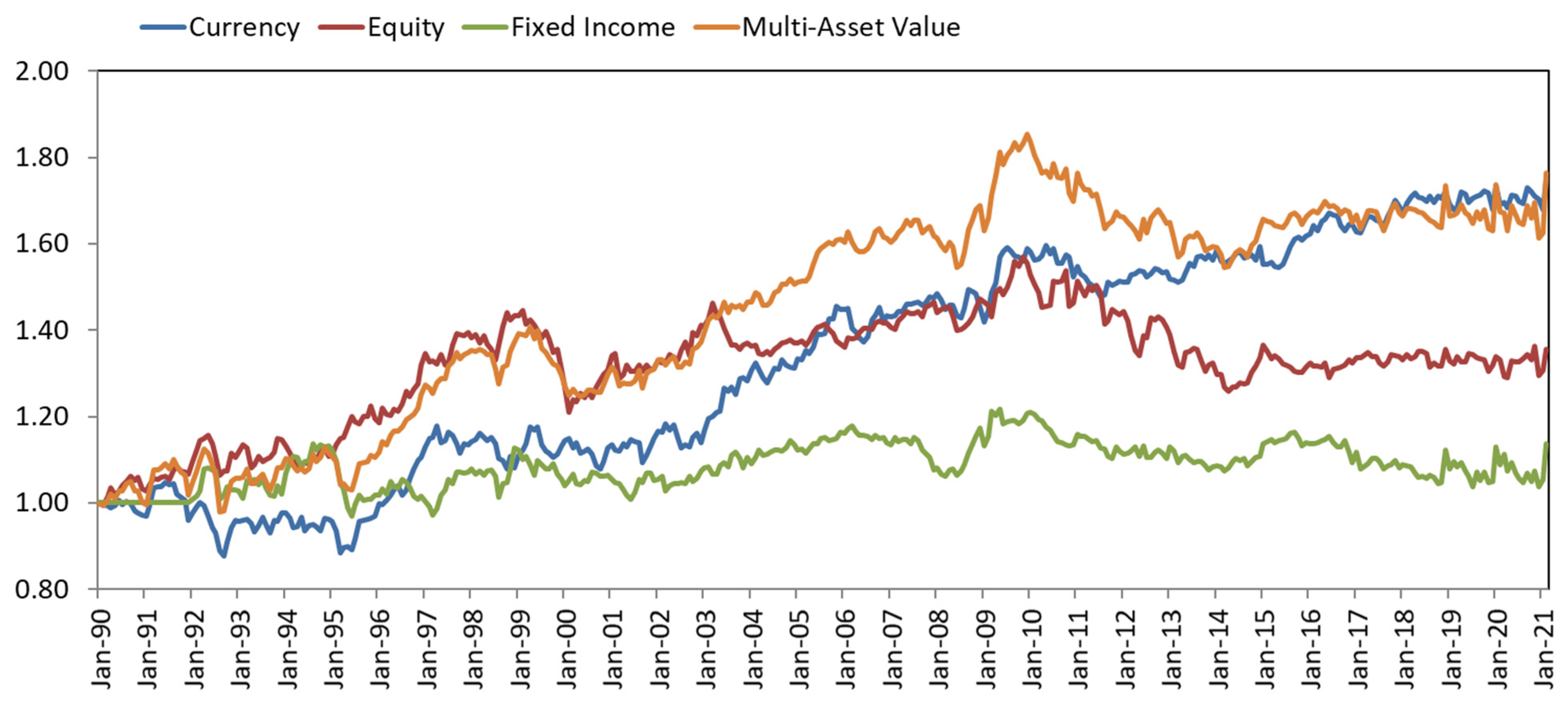
The last decade was challenging for multi-asset value portfolios.
Figure 1 shows the historical cumulative returns in value for bonds, currencies, country equities, and diversified multi-asset value portfolios in developed markets from 1990 through February 2021.
The figure shows the cumulative gross returns for value strategies in developed currencies (currency), developed country equities (equity), developed country bonds (fixed income), and developed diversified multi-asset portfolios (multi-asset value). Statistics are computed from monthly return series over the sample time period: January 1990–February 2021. For developed country bonds, the sample time period is January 1991–February 2021. Portfolios are rebalanced monthly. Weights are scaled so that the ex-post volatility of each strategy is set to 5% over the entire backtest period for comparison purposes. Reported returns do not include transaction costs.
While the diversified multi-asset value portfolio had positive performance in the early years, it generated a substantial loss over the most recent decade.
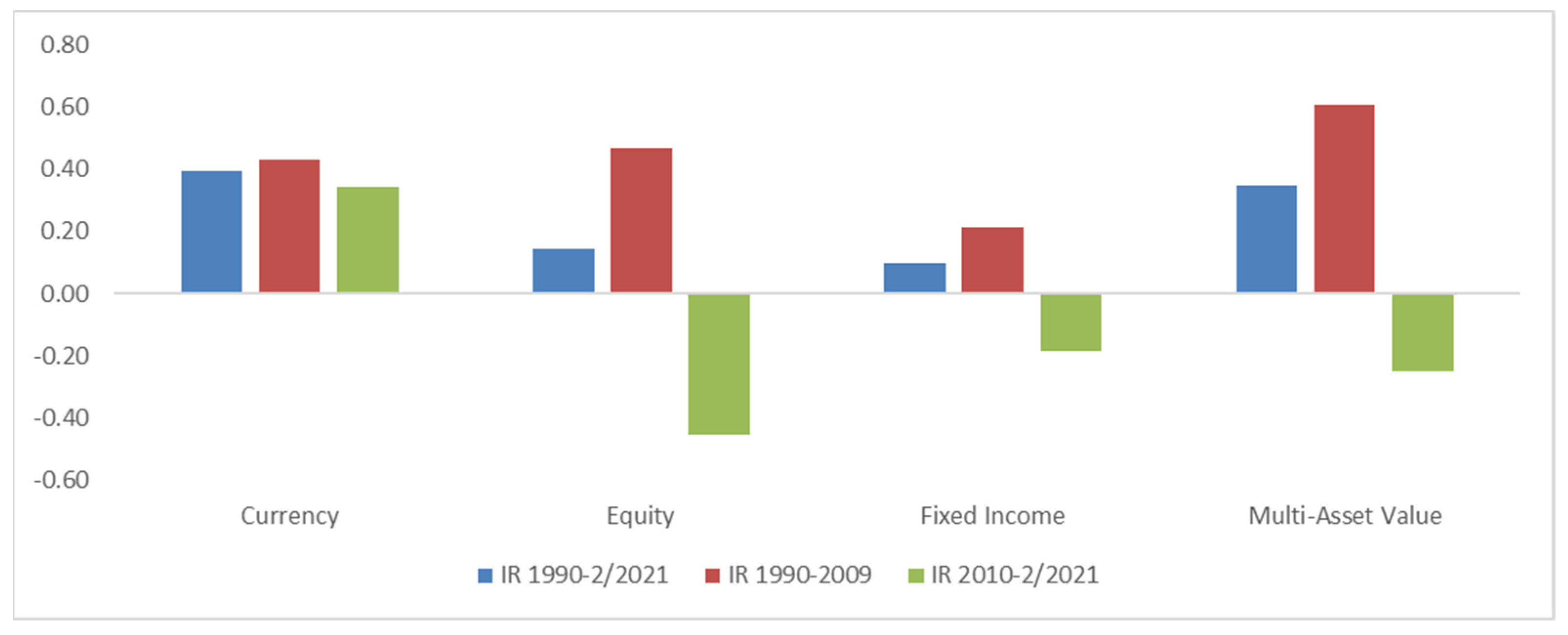
To shed more light on these findings,
Figure 2 compares the performance of value portfolios in the last decade vs. the historical averages computed from January 1990 to December 2009. The diversified multi-asset value portfolio realized a negative information ratio in this recent time period (−0.25), compared to a positive one (0.61) in the earlier period. There are significant differences when observing the asset class-specific value portfolios. Developed fixed income and country equities value portfolios earned negative returns, while developed currency portfolios realized risk-adjusted returns comparable to earlier time periods.
The figure shows the information ratio (IR) for value strategies in developed currencies (currency), developed country equities (equity), developed country bonds (fixed income), and developed diversified multi-asset portfolios (multi-asset value). Statistics are computed from a monthly return series over the sample time period: January 1990–February 2021. For developed country bonds, the sample time period is January 1991–February 2021. Portfolios are rebalanced monthly. Weights are scaled so that the ex-post volatility of each strategy is set to 5% over the entire backtest period for comparison purposes. Reported returns do not include transaction costs.
5. Value Factor Payoff and the Global Business Cycle
The literature (
Kolanovic and Wei 2013;
Ilmanen et al. 2019;
Bellone et al. 2019) has sought to link the value payoff to global inflation and real growth, with mixed results. To explore whether or not the value payoff varies with the global business cycle, we conducted a linear regression analysis of the value payoff in developed currencies, bonds, and country equities on global consensus inflation and real growth expectations.
In
Table 4, we find weak negative exposure to real growth in currencies and fixed income, and an equal risk composite has a nonstatistically negative exposure to real growth. This relationship is not very strong, as the
R2 of the regression is only 1%. In addition, inflation regression results have no statistical significance across all universes.
The table reports a linear regression of expected global real growth or inflation onto returns of value strategies in developed currencies (currency), developed country equities (equity), developed country bonds (fixed income), and developed diversified multi-asset portfolios (multi-asset value). For developed markets equities and currencies, the sample time period is January 1990–February 2021. For developed country bonds, the sample time period is January 1991–February 2021. Portfolios are rebalanced monthly. Significance at the 1% level is denoted in bold, while significance at the 10% level is denoted in bold and italics.
It is possible that the relationship between the value factor payoff and global growth is nonlinear and cannot be captured in a simple linear regression. To explore this relationship nonparametrically, we divided the global growth environment into four quartiles and computed the average payoff in each state. While there is no strong pattern,
Table 5 shows weak support for the assertion that value has historically done better in the lowest global growth environments. This is also supportive of the linear regression results that show value is weakly countercyclical.
Information ratios (IR) are reported for value strategies in developed currencies (currency), developed country equities (equity), developed country bonds (fixed income), and developed diversified multi-asset portfolios (multi-asset value). Statistics are computed from a monthly return series over the sample time period: January 1990–February 2021. For developed country bonds, the sample time period is January 1991–February 2021. Portfolios are rebalanced monthly. Weights are scaled so that the ex-post volatility of each strategy is set to 5% over the entire backtest period for comparison purposes. Reported returns do not include transaction costs.
6. Revealing the Macro Characteristics of Value Portfolios
The literature (
Ilmanen et al. 2019;
Bellone et al. 2019) has sought to link the value payoff to global inflation and real growth. To check this assertion, we measured the net inflation and real growth characteristics directly from the holdings of the value portfolio by borrowing the framework introduced by
Zangari (
2003), applied to multi-asset carry portfolios by
Aiolfi and Tokat-Acikel (
2019). Taking advantage of the cross-country inflation and growth expectations implicit in every value portfolio, we multiplied country weights in the portfolio by their forecasted rates of inflation and real GDP, to derive the net inflation and real growth characteristics embedded in each asset class value portfolio at each point in time. This approach allows us to derive a time series of the macro characteristics of value portfolios that we can then use to estimate the average macro characteristics over our full analysis period.
Consider a simplified currency value portfolio that is long Japanese yen and short Australian dollars. This portfolio is mapped to: (1) long Japanese inflation expectations and short Australian inflation expectations, and (2) long Japanese real growth expectations and short Australian real growth expectations. If Japanese real growth (or inflation) expectations end up being higher than Australian real growth (or inflation) expectations, then the currency value portfolio will show net positive real growth (or inflation) characteristics.
The remainder of this section is organized as follows. First, we estimate the average net growth and inflation exposures embedded in each value portfolio and study the time-series behavior of such exposures. Next, we examine whether the time-varying macroeconomic exposures embedded in value portfolios can explain the returns to value strategies. Finally, we use a closely related but different methodology to show that the payoff to value portfolios in various asset classes are linked to relative growth and inflation expectations across countries.
6.1. Net Growth and Inflation Characteristics in Value Portfolios
We define the real GDP growth exposures of the value portfolio
at time
as:
where
is the weight of asset
in asset class
at time
and
is the real GDP forecast for country
at time
. Note that there is a one-to-one mapping between asset
i and country
for each asset class
. For example, the Australian dollar, government bond, and country equities are all linked to Australian inflation and real growth expectations. The weight of Australia in a currency, bond, or equity value portfolio depends on how attractive it is relative to other countries in that universe, based on the value factor used. A similar exercise using inflation forecasts allows us to define the inflation characteristics of a given value portfolio.
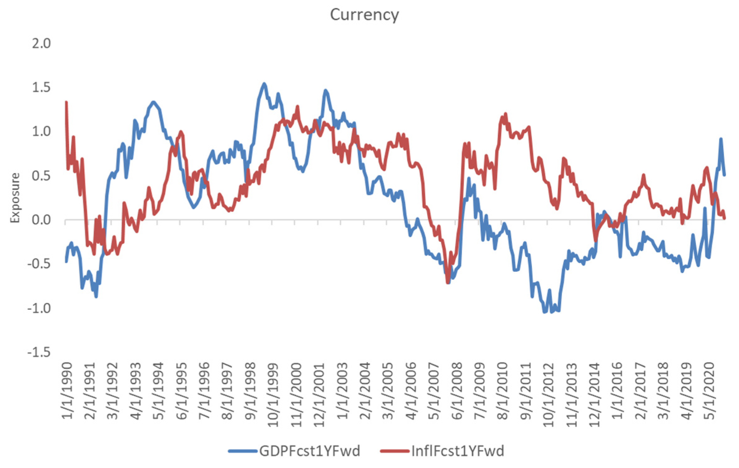
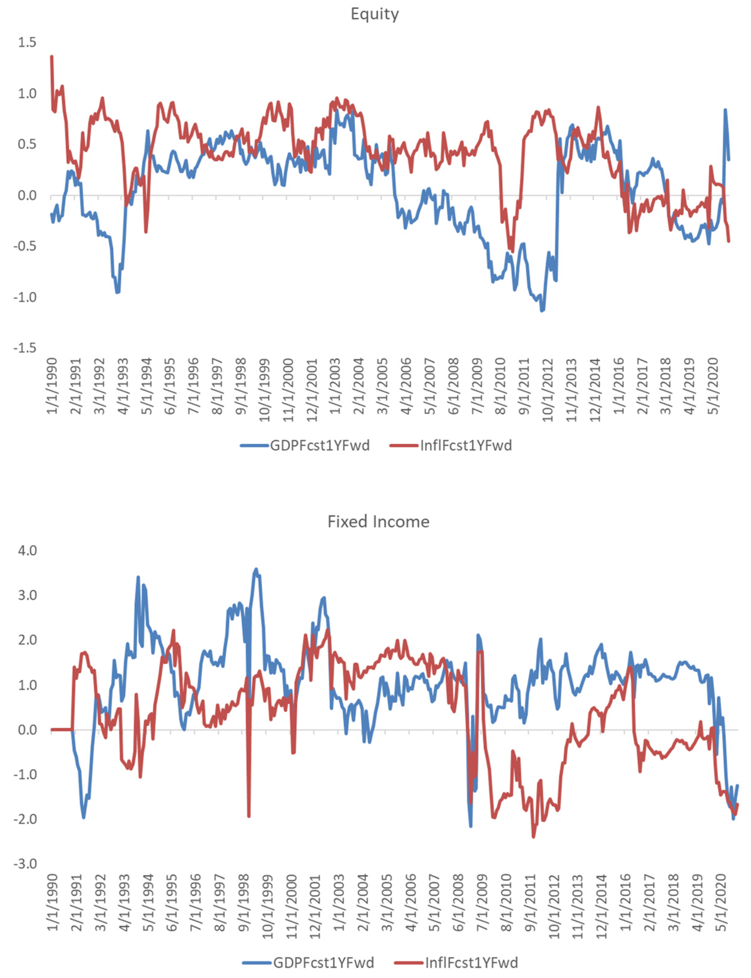
Figure 3 shows that the inflation and real growth characteristics of developed currency, equity, and fixed income value portfolios have varied over time. Inflation characteristics of value portfolios in developed currencies have been positive and fairly stable through time, while growth characteristics have behaved somewhat differently, turning negative from 2010 through 2020. Other asset classes show different time-series behavior in their inflation and growth characteristics, suggesting once more that these portfolios have only a very small systematic component in common.
The figure shows inflation and real growth exposures of developed currency value portfolios (currency) developed country equities (equity), and developed country bonds (fixed income). Statistics are computed from monthly series over the sample time period: January 1990–February 2021. Portfolios are rebalanced monthly.
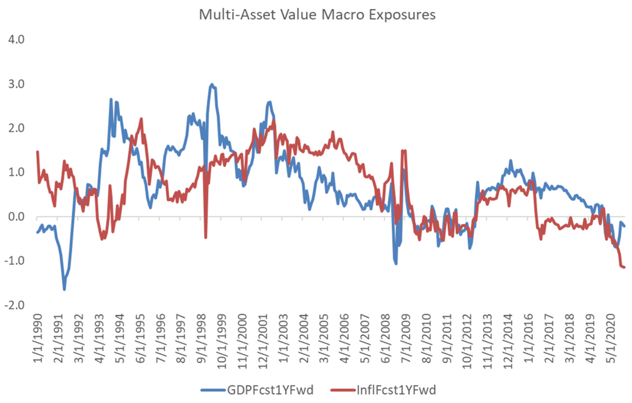
Figure 4 shows similar results for a diversified multi-asset value portfolio. Real growth and inflation characteristics of value were generally positive and relatively stable in earlier periods. The only exceptions were the negative exposures to both real growth and inflation during the early 1990s and the Global Financial Crisis of 2008, as well as the more recent negative exposure to inflation.
The figure shows growth and inflation exposures of developed diversified multi-asset portfolios (multi-asset value). Statistics are computed from monthly series over the sample time period: January 1990–February 2021. Portfolios are rebalanced monthly.
While the time-series variation in the characteristics of value portfolios is interesting, we also want to estimate the average expected nominal growth exposure of value portfolios.
Table 6 shows that the average growth and inflation expectations (in percentages) embedded in value portfolios are positive and statistically significant across different asset classes. This differs notably from the stock selection literature that shows value stock portfolios load negatively on growth (
Fama and French 1992).
7Exposure statistics for expected real growth and inflation (in percentages) are reported among value strategies in developed currencies (currency), developed country equities (equity), developed country bonds (fixed income), and developed diversified multi-asset portfolios (multi-asset value). Statistics are computed from a monthly series over the sample time period: January 1990–February 2021. For developed country bonds, the sample time period is January 1991–February 2021. Portfolios are rebalanced monthly.
6.2. Can the Value Payoff Be Explained by Macro Exposures?
Now that we have a more precise way of determining the portfolio’s macro characteristics, we can explore the time-varying macro exposures, and whether or not they can explain the time-varying payoff to value portfolios. To do so, we first use the embedded macro characteristics of value portfolios to conduct a simple nonparametric analysis and study the behavior of the value payoff during periods of higher (lower) than average real growth and inflation exposures. The results in
Table 7 (A) show that a diversified multi-asset value portfolio produces better risk-adjusted returns when both net real growth and inflation exposures (namely nominal growth) were higher than average. When we break the analysis down to only real growth or inflation states, the results are a bit more mixed. In country equities and currencies, higher net growth and inflation spreads tend to be positively related to a higher payoff in value. In cross-country fixed income value portfolios, the opposite is true. Moreover, we notice once more that value in currencies displays a subtler cycle of performance across different regimes in macro characteristics. Both of these findings are in line with the positive correlation of fixed income value with fixed income benchmarks, and currency value with the US dollar index reported in
Table 2.
Performance statistics are reported for value strategies in developed currencies (currency), developed country equities (equity), developed country bonds (fixed income), and developed diversified multi-asset portfolios (multi-asset value). Statistics are computed from a monthly return series over the sample time period: January 1990–February 2021. For developed country bonds, the sample time period is January 1991–February 2021. Portfolios are rebalanced monthly. Weights are scaled so that the ex-post volatility of each strategy is set to 5% over the entire backtest period for comparison purposes. Reported returns do not include transaction costs.
We can now conduct a more formal regression analysis, relating returns of the value factor payoff to net growth and inflation exposures in the portfolio in
Table 8. For each asset class, we regress the value payoff on the net real growth and inflation exposures derived in the prior section:
This analysis confirms the directionality of the results shown in
Table 7. Across asset classes, the betas to macro characteristics are generally positive, but only weakly statistically significant. While economic significance is not trivial, the statistical significance is weak. Given the low explanatory power of the regressions, we do not find evidence for explaining value portfolios using their time-varying exposures to expect real growth and inflation.
Table 8.
Value portfolio payoff regression on net expected inflation or growth in the portfolio (1/1990–2/2021).
Table 8.
Value portfolio payoff regression on net expected inflation or growth in the portfolio (1/1990–2/2021).
| | Currency | Equity | Fixed Income | Multi-Asset Value |
|---|
| cGDP | 0.140 | 0.047 | 0.091 | 0.001 |
| BetaGDP | 0.057 | 0.162 | −0.128 | 0.208 |
| R2 | 0.00 | 0.00 | 0.01 | 0.00 |
| cInfl | 0.088 | −0.008 | 0.030 | 0.000 |
| BetaInfl | 0.153 | 0.161 | −0.042 | 0.441 |
| R2 | 0.00 | 0.00 | 0.00 | 0.01 |
The table reports the linear regression of net expected real growth or inflation exposures onto returns of value strategies in developed currencies (currency), developed country equities (equity), developed country bonds (fixed income), and developed diversified multi-asset portfolios (multi-asset value). For developed markets equities and currencies, the sample time period is January 1990–February 2021. For developed country bonds, the sample time period is January 1991–February 2021. Portfolios are rebalanced monthly. Significance at the 1% level is denoted in bold, while significance at the 10% level is denoted in bold and italics.
6.3. Value Portfolios Are Proxies for Rankings on Country Growth and Inflation
It is typical to find weak relationships between returns and macro fundamentals, as net growth and inflation exposures are very slow-moving, while returns are highly variable.
Aiolfi and Tokat-Acikel (
2019) propose an alternate way of linking these by constructing factor-mimicking macro portfolios. Following this approach, we construct factor-mimicking portfolios for growth and inflation, then we calculate the return on these portfolios. Once the factor payoff is observable, we can estimate the exposures of the individual value portfolio to the factor-mimicking portfolio. Using the same portfolio construction approach discussed in
Section 3.4, we rank each country’s equity, currency, or bond market based on its inflation and real growth at each point in time and build dollar-neutral long–short portfolios by weighting securities in a linear fashion.
We perform the following regression analysis to explain the payoff of asset class-specific value portfolios using asset class-specific inflation or growth factor-mimicking portfolios:
where
is the return of the value factor portfolio in asset class
j at time
t,
is the return of the real growth factor-mimicking portfolio in asset class
j at time
t, and
is the return of the inflation factor-mimicking portfolio in asset class
j at time
t.
Through this type of factor-mimicking portfolio, we find that the payoff in value portfolios in various asset classes is linked to relative growth and inflation expectations across countries. Our regression of the value payoff against the relative growth and inflation payoffs in
Table 9 yields statistically and economically significant betas from 1990 through February 2021.
Value-ranked portfolios in developed currencies, bonds, and equities essentially rank assets based on country inflation and growth expectations. While these value portfolios trade different assets, they share the same macro exposures, overweighting countries with higher inflation and growth expectations. The only exception is the country equities value portfolio, which has a negative beta to the payoff of the growth factor-mimicking portfolio, suggesting a slightly countercyclical behavior.
In terms of economic significance, our analysis shows that a diversified multi-asset value portfolio enjoys a 37 bps (71 bps) increase in returns if the payoff of the growth (inflation) factor-mimicking portfolio increases by 1%.
Table 9.
Value portfolio payoff regression on growth and inflation factor-mimicking portfolio payoff (1/1990–2/2021).
Table 9.
Value portfolio payoff regression on growth and inflation factor-mimicking portfolio payoff (1/1990–2/2021).
| | Currency | Equity | Fixed Income | Multi-Asset Value |
|---|
| cFGDP | 0.111 | 0.055 | 0.032 | 0.001 |
| BetaGDP | 0.447 | −0.112 | 0.446 | 0.367 |
| R2 | 0.23 | 0.01 | 0.26 | 0.03 |
| cFInfl | 0.116 | 0.006 | 0.018 | 0.001 |
| BetaInfl | 0.252 | 0.353 | 0.313 | 0.712 |
| R2 | 0.07 | 0.11 | 0.13 | 0.08 |
The table reports the linear regression of factor-mimicking returns for real growth or inflation onto returns of value strategies in developed currencies (currency), developed country equities (equity), developed country bonds (fixed income), and developed diversified multi-asset portfolios (multi-asset value). For developed market equities and currencies, the sample time period is January 1990–February 2021. For developed country bonds, the sample time period is January 1991–February 2021. Portfolios are rebalanced monthly. Significance at the 1% level is denoted in bold, while significance at the 10% level is denoted in bold and italics.
7. Value Characteristics since the Global Financial Crisis: Has Anything Changed?
We repeat the factor-mimicking portfolio returns analysis we conducted in
Section 6.3 for the first two decades of our sample (1990–2009), as well as post-2010 to explore if we can provide any explanation for weak value factor performance since the GFC.
Table 10 shows that between 1990 and 2009, value portfolios had a significant positive beta to inflation and growth factor-mimicking portfolios (Panel A), while post-2009, the same betas turned negative (Panel B). The implication is that post-2009, value-ranked portfolios were overweighting countries with relatively lower growth and inflation exposures compared to two decades prior. This change in macro characteristics coincides with the period of unconventional central bank policies designed to lift global growth after the GFC. Because of concerns over low rates and slow global growth after the GFC, investors became willing to pay for scarce growth, while cheaper assets from countries with lower growth prospects have not been rewarded by markets over the recent decade. In fact, this does not seem to be in conflict with history. Our prior analysis in
Section 6.2 shows that the payoff to valuation factors was historically stronger when the net growth exposure was high.
This table reports the linear regression of factor-mimicking returns for real growth or inflation onto returns of value strategies in developed currencies (currency), developed country equities (equity), developed country bonds (fixed income), and developed diversified multi-asset portfolios (multi-asset value). For developed market equities and currencies, the sample time period is January 1990–February 2021. For developed country bonds, the sample time period is January 1991–February 2021. Portfolios are rebalanced monthly. Significance at the 1% level is denoted in bold, while significance at the 10% level is denoted in bold and italics.
8. Conclusions
Value factor portfolios have struggled across asset classes over the last decade. Our novel approach to identifying the underlying macroeconomic characteristics of value factor portfolios through the use of holdings-based and factor-mimicking portfolio analyses provided unique insights. In addition to determining the typical, or average, characteristics, we can estimate the macroeconomic characteristics of portfolio holdings at any given point in time. We found that value portfolios have historically provided exposure to countries with relatively higher inflation or growth. Our analysis suggests that recent value underperformance was idiosyncratic, not cyclical. Time variation did not help to explain the variation in the value payoff. However, we found that relatively cheaper assets had much lower growth and inflation exposures after 2009 when compared to earlier decades. We are uncertain if these changes were secular, or due to a factor payoff cycle. This characteristic coincided with the period of unconventional central bank policies designed to lift global growth after the Global Financial Crisis. Concerns over low rates and slow global growth post-GFC caused investors to become willing to pay for scarce growth, while cheaper assets from countries with lower growth prospects were not rewarded by markets over the last decade. The COVID-19 pandemic in 2020 created significant economic disruption that was met with swift fiscal and monetary response. Longer term impact of this crisis on value factor payoff is not yet clear.
Author Contributions
Conceptualization, Y.T.-A. and M.A.; methodology, Y.T.-A. and M.A.; software, Y.J.; validation Y.T.-A., M.A., and Y.J.; formal analysis Y.J.; investigation Y.J.; resources, Y.T.-A. and M.A.; data curation, Y.J.; writing—original draft preparation, Y.T.-A. and M.A.; writing—review and editing, Y.T.-A. and M.A.; visualization, Y.J.; supervision, Y.T.-A. and M.A.; project administration, Y.T.-A. and M.A.; funding acquisition, Y.T.-A. and M.A. All authors have read and agreed to the published version of the manuscript.
Funding
This research received no external funding.
Data Availability Statement
The data presented in this study are available on request from the corresponding author. The data are not publicly available due to privacy.
Acknowledgments
We would like to thank Roy Henriksson, George Sakoulis, Lorne Johnson, Weijian Liang, and Edward Tostanoski for their feedback on earlier versions of this paper. These materials represent the views and opinions of the authors regarding the economic conditions, asset classes, or financial instruments referenced herein and are not necessarily the views of PGIM Quantitative Solutions.
Conflicts of Interest
The authors declare no conflict of interest.
Abbreviations
PGIM Quantitative Solutions is a wholly-owned subsidiary of PGIM, Inc., the principal asset management business of Prudential Financial Inc. of the United States of America.
Notes
| 1 | |
| 2 | See Florian Steiger ( 2010), “The Validity of Company Valuation Using Discounted Cash Flow Methods”. |
| 3 | Various international agencies, such as the OECD and IMF as well as many private banks and financial institutions, such as The Economist magazine, compute PPP indices for most countries. |
| 4 | MSCI has not approved, reviewed, or produced this report, makes no express or implied warranties or representations and is not liable whatsoever for any data in the report. You may not redistribute the MSCI data or use it as a basis for other indices or investment products. |
| 5 | We used approximate GDP weights for G7 countries. The weights were as follows: Unites States 52.7%, Japan 13.7%, Germany 9.7%, United Kingdom 7.4%, France 7.0%, Italy 5.3%, Canada 4.2%. |
| 6 | We also created global growth and inflation forecasts using equal weighting 7 major developed countries’ growth and inflation forecast. All reported results are robust to the weighting scheme for global growth or inflation. Results are available upon request. |
| 7 | To address this shortcoming in practice, index providers such as MSCI have started using valuation as well as growth factors, such as earnings growth, to classify stocks in their value and growth indices. |
| 8 | The average nominal growth net exposures are as follows: Currency 0.63, Equity 0.47, Fixed Income 1.38, Multi-Asset Value portfolio 1.34. |
| 9 | The average real growth net exposures are as follows: Currency 0.19, Equity 0.05, Fixed Income 1.04, Multi-Asset Value portfolio 0.70. |
| 10 | The average inflation net exposures are as follows: Currency 0.44, Equity 0.42, Fixed Income 0.34, Multi-Asset Value portfolio 0.65. |
References
- Abuaf, Niso, and Philippe Jorion. 1990. Purchasing Power Parity in the Long Run. The Journal of Finance 45: 157–74. [Google Scholar] [CrossRef]
- Aiolfi, Marco, and Yesim Tokat-Acikel. 2019. Don’t Get Carried Away: Uncovering Macro Characteristics in Carry Portfolios. Journal of Investment Management 17. [Google Scholar] [CrossRef]
- Aked, Michael, Brandon Kunz, and Amie Ko. 2018. Alternative Risk Premia: Crisis or Opportunity? Newport Beach: Research Affiliates, Newport Beach. [Google Scholar]
- Arnott, Rob, Campbell R. Harvey, Vitali Kalesnik, and Juhani Linnainmaa. 2019. Alice’s Adventures in Factorland: Three Blunders that Plague Factor Investing. The Journal of Portfolio Management 45: 18–36. [Google Scholar] [CrossRef] [Green Version]
- Asness, Clifford S., Antti Ilmanen, Ronen Israel, and Tobisa Moskowitz. 2015. Investing with Style. Journal of Investment Management 13: 27–63. [Google Scholar]
- Asness, Clifford S., Tobias J. Moskowitz, and Lasse Heje Pedersen. 2013. Value and Momentum Everywhere. The Journal of Finance 68: 929–85. [Google Scholar] [CrossRef] [Green Version]
- Baltussen, Guido, Laurens Swinkels, and Pim Van Vliet. 2019. Global Factor Premiums. Available online: https://www.sciencedirect.com/science/article/pii/S0304405X21003007?via%3Dihub (accessed on 15 May 2021).
- Baz, Jamil, Nicolas Granger, Campbell R. Harvey, Nicolas Le Roux, and Sandy Rattray. 2015. Dissecting Investment Strategies in the Cross Section and Time Series. Available online: https://papers.ssrn.com/sol3/papers.cfm?abstract_id=2695101 (accessed on 15 May 2021).
- Bellone, Benoit, Philippe Declerck, Mounir Nordine, and Thomas Vy. 2019. Multi-Asset Style Factors Have Their Shining Moments. Available online: https://papers.ssrn.com/sol3/Papers.cfm?abstract_id=3444208 (accessed on 15 May 2021).
- Fama, Eugene F., and Kenneth R. French. 1992. The Cross-Section of Expected Stock Returns. The Journal of Finance 47: 427–65. [Google Scholar] [CrossRef]
- Flood, Robert P., and Mark P. Taylor. 1996. Exchange Rate Economics: What’s Wrong with the Conventional Macro Approach? In The Microstructure of Foreign Exchange Markets. Chicago: University of Chicago Press. [Google Scholar]
- Ilmanen, Antti, Ronen Israel, Tobias J. Moskowitz, Ashwin K. Thapar, and Franklin Wang. 2019. Factor Premia and Factor Timing: A Century of Evidence. Working Paper. Greenwich: AQR Capital Management. [Google Scholar]
- Imbs, Jean, Haroon Mumtaz, Morten O. Ravn, and Hélène Rey. 2005. PPP Strikes Back: Aggregation and the Real Exchange Rate. The Quarterly Journal of Economics 120: 1–43. [Google Scholar]
- Koijen, Ralph S. J., Tobias J. Moskowitz, Lasse Heje Pedersen, and Evert B. Vrugt. 2018. Carry. Journal of Financial Economics 127: 197–225. [Google Scholar] [CrossRef] [Green Version]
- Kolanovic, Marko, and Zhen Wei. 2013. Systematic Strategies across Asset Classes: Risk Factor Approach to Investing and Portfolio Management. JP Morgan Global Quantitative and Derivate Strategy, 1–205. [Google Scholar]
- Lakonishok, Josef, Andrei Shleifer, and Robert W. Vishny. 1994. Contrarian Investment, Extrapolation, and Risk. The Journal of Finance 49: 1541–78. [Google Scholar] [CrossRef]
- Lakos-Bujas, Dubravko, Narendra Singh, Arun Jain, Bhupinder Singh, Kamal Tamboli, and Marko Kolanovic. 2019. The Value Conundrum. New York: J.P. Morgan, Equity Strategy and Quantitative Research. [Google Scholar]
- Petkova, Ralitsa, and Lu Zhang. 2005. Is Value Riskier Than Growth? Journal of Financial Economics 78: 187–202. [Google Scholar] [CrossRef]
- Singh, Jyoti, Gavin Smith, and Peter Xu. 2019. Is The Price Right? Drivers of Value Factor Performance. Newark: PGIM Quantitative Solutions. [Google Scholar]
- Steiger, Florian. 2010. The Validity of Company Valuation Using Discounted Cash Flow Methods. arXiv arXiv:1003.4881. [Google Scholar]
- Yara, Fahiz Baba, Martijn Boons, and Andrea Tamoni. 2019. Value Return Predictability across Asset Classes and Commonalities in Risk Premia. Review of Finance 25: 449–84. [Google Scholar] [CrossRef]
- Zangari, Peter. 2003. Equity Risk Factor Models. In Bob Litterman and the Quantitative Resources Group of Goldman Sachs Asset Management, Modern Investment Management. Hoboken: John Wiley & Sons. [Google Scholar]
Figure 1.
Simulated cumulative returns of value strategies across asset classes. Sources: PGIM Quantitative Solutions, MSCI, WMR, Bloomberg.
Figure 1.
Simulated cumulative returns of value strategies across asset classes. Sources: PGIM Quantitative Solutions, MSCI, WMR, Bloomberg.
Figure 2.
Information ratio of value strategies across asset classes. Sources: PGIM Quantitative Solutions, MSCI, WMR, Bloomberg.
Figure 2.
Information ratio of value strategies across asset classes. Sources: PGIM Quantitative Solutions, MSCI, WMR, Bloomberg.
Figure 3.
Macroeconomic characteristics of value portfolios. Sources: PGIM Quantitative Solutions, MSCI, WMR, Bloomberg, Consensus Economics.
Figure 3.
Macroeconomic characteristics of value portfolios. Sources: PGIM Quantitative Solutions, MSCI, WMR, Bloomberg, Consensus Economics.
Figure 4.
Macroeconomic characteristics of diversified multi-asset value portfolios. Sources: PGIM Quantitative Solutions, MSCI, WMR, Bloomberg, Consensus Economics.
Figure 4.
Macroeconomic characteristics of diversified multi-asset value portfolios. Sources: PGIM Quantitative Solutions, MSCI, WMR, Bloomberg, Consensus Economics.
Table 1.
An example of long–short value portfolio for fixed income (as of 2/2021).
Table 1.
An example of long–short value portfolio for fixed income (as of 2/2021).
| Fixed Income Assets | EUBond | JPBond | UKBond | USBond | AUBond | CABond |
|---|
| Real Yield (%) | −1.93 | 0.22 | −1.74 | −0.84 | 0.19 | −0.39 |
| Asset Rank | 1 | 6 | 2 | 3 | 5 | 4 |
| Rescaled Asset Weight | −73.66% | 73.66% | −44.20% | −14.73% | 44.20% | 14.73% |
Table 2.
Performance of value across asset classes (1/1990–2/2021).
Table 2.
Performance of value across asset classes (1/1990–2/2021).
| | Currency | Equity | Fixed Income | Multi-Asset Value |
|---|
| Observations | 374 | 374 | 362 | 374 |
| Geometric Mean | 1.8% | 1.0% | 0.5% | 1.9% |
| Vol | 5.0% | 5.0% | 5.0% | 5.0% |
| IR 1/1990–2/2021 | 0.39 | 0.14 | 0.11 | 0.35 |
| Corr (MSCI ACWI) | 0.04 | 0.02 | 0.05 | 0.05 |
| Corr (Fixed Income) | −0.08 | 0.02 | −0.16 | −0.13 |
| Corr (DXY) | 0.42 | −0.06 | −0.04 | 0.17 |
| Skew | −0.17 | −0.27 | 0.07 | −0.51 |
| Excess Kurtosis | 1.30 | 1.12 | 1.91 | 2.58 |
Table 3.
Correlations of value portfolios across asset classes (1/1990–2/2021).
Table 3.
Correlations of value portfolios across asset classes (1/1990–2/2021).
| | Currency | Equity | Fixed Income |
|---|
| Currency | 1.00 | 0.02 | 0.12 |
| Equity | | 1.00 | 0.03 |
| Fixed Income | | | 1.00 |
Table 4.
Value portfolio payoff regression on expected global inflation or growth (1/1990–2/2021).
Table 4.
Value portfolio payoff regression on expected global inflation or growth (1/1990–2/2021).
| | Currency | Equity | Fixed Income | Multi-Asset Value |
|---|
| cGDP | 0.459 | 0.001 | 0.138 | 0.004 |
| BetaGDP | −0.149 | 0.025 | −0.056 | −0.127 |
| R2 | 0.01 | 0.00 | 0.00 | 0.01 |
| cInfl | 0.340 | −0.176 | 0.021 | 0.001 |
| BetaInfl | −0.092 | 0.111 | 0.001 | 0.004 |
| R2 | 0.00 | 0.00 | 0.00 | 0.00 |
Table 5.
Performance of value in different growth states (1/1990–2/2021).
Table 5.
Performance of value in different growth states (1/1990–2/2021).
| Global Growth Percentiles | Currency | Equity | Fixed Income | Multi-Asset Value |
|---|
| Q1 (G > 75% pctl) | 0.10 | 0.54 | −0.07 | 0.41 |
| Q2 (75% pctl > G > 50% pctl) | −0.15 | −0.33 | −0.18 | −0.34 |
| Q3 (50% pctl > G > 25% pctl) | 0.75 | 0.87 | 0.38 | 0.14 |
| Q4 (G < 25% pctl) | 0.88 | 0.71 | 0.00 | 0.33 |
Table 6.
Average macroeconomic characteristics of developed value portfolios (1/1990–2/2021).
Table 6.
Average macroeconomic characteristics of developed value portfolios (1/1990–2/2021).
| | GDPFcst1YFwd | |
| 1990–2/2021 | Currency | Equity | Fixed Income | Multi-Asset Value |
| Avg | 0.19 | 0.05 | 1.04 | 0.70 |
| t-stat | 5.62 | 2.18 | 21.52 | 16.16 |
| 5th Perc | −0.72 | −0.82 | −0.80 | −0.56 |
| 95th Perc | 1.29 | 0.63 | 2.70 | 2.26 |
| | InflFcst1YFwd | |
| 1990–2/2021 | Currency | Equity | Fixed Income | Multi-Asset Value |
| Avg | 0.44 | 0.42 | 0.34 | 0.65 |
| t-stat | 19.92 | 24.13 | 5.91 | 16.70 |
| 5th Perc | −0.29 | −0.22 | −1.70 | −0.45 |
| 95th Perc | 1.08 | 0.89 | 1.82 | 1.82 |
Table 7.
Performance of value in higher/lower-than-average net growth and inflation exposures (1/1990–2/2021).
Table 7.
Performance of value in higher/lower-than-average net growth and inflation exposures (1/1990–2/2021).
| A Value Portfolio IR (1/1990–2/2021) |
| | Currency | Equity | Fixed Income | Multi-Asset Value |
| NGDP Exposure > Avg8 | 0.54 | 0.39 | −0.04 | 0.80 |
| NGDP Exposure < Avg | 0.20 | −0.12 | 0.24 | 0.00 |
| B Value Portfolio IR (1/1990–2/2021) |
| | Currency | Equity | Fixed Income | Multi-Asset Value |
| GDP Exposure > Avg9 | 0.43 | 0.28 | −0.23 | 0.72 |
| GDP Exposure < Avg | 0.38 | −0.02 | 0.57 | 0.08 |
| C Value Portfolio IR (1/1990–2/2021) |
| | Currency | Equity | Fixed Income | Multi-Asset Value |
| Infl Exposure > Avg10 | 0.45 | 0.35 | −0.06 | 0.67 |
| Infl Exposure < Avg | 0.34 | −0.15 | 0.25 | 0.07 |
Table 10.
Value portfolio payoff regression on growth and inflation factor-mimicking portfolio payoff.
Table 10.
Value portfolio payoff regression on growth and inflation factor-mimicking portfolio payoff.
| A. Value Portfolio Payoff Regression on Growth and Inflation Factor-Mimicking Portfolio Payoff (1/1990–12/2009). |
| | Currency | Equity | Fixed Income | Multi-Asset Value |
| cFGDP | 0.001 | 0.002 | 0.001 | 0.003 |
| BetaGDP | 0.677 | 0.057 | 0.428 | 0.319 |
| R2 | 0.46 | 0.00 | 0.24 | 0.10 |
| cFInfl | 0.001 | 0.001 | 0.001 | 0.002 |
| BetaInfl | 0.345 | 0.438 | 0.390 | 0.397 |
| R2 | 0.12 | 0.19 | 0.21 | 0.17 |
| B. Value Portfolio Payoff Regression on Growth and Inflation Factor-Mimicking Portfolio Payoff (1/2010–2/2021). |
| | Currency | Equity | Fixed Income | Multi-Asset Value |
| cFGDP | 0.097 | −0.135 | −0.042 | 0.000 |
| BetaGDP | −0.273 | −0.409 | 0.537 | −0.702 |
| R2 | 0.15 | 0.17 | 0.36 | 0.11 |
| cFInfl | 0.079 | −0.169 | −0.025 | −0.001 |
| BetaInfl | −0.045 | 0.064 | −0.042 | −0.358 |
| R2 | 0.00 | 0.00 | 0.00 | 0.02 |
| Publisher’s Note: MDPI stays neutral with regard to jurisdictional claims in published maps and institutional affiliations. |
© 2021 by the authors. Licensee MDPI, Basel, Switzerland. This article is an open access article distributed under the terms and conditions of the Creative Commons Attribution (CC BY) license (https://creativecommons.org/licenses/by/4.0/).


