Communication

True versus Spurious Long Memory in Cryptocurrencies

by
Dooruj Rambaccussing
* and
Murat Mazibas
School of Business, University of Dundee, Dundee DD1 3BH, UK
*
Author to whom correspondence should be addressed.
J. Risk Financial Manag. 2020, 13(9), 186; https://doi.org/10.3390/jrfm13090186
Submission received: 22 July 2020 / Revised: 14 August 2020 / Accepted: 17 August 2020 / Published: 19 August 2020

Abstract

:
We test whether the selected cryptocurrencies exhibit long memory behavior in returns and volatility. We use data on five most traded cryptocurrencies: Bitcoin, Litecoin, Ethereum, Bitcoin Cash, and XRP. Using recent tests of long memory developed against persistent and nonlinear alternatives, this paper finds that long memory is mostly rejected in returns. The tests fail to reject the null hypothesis of long memory in most cases across different volatility proxies and cryptocurrencies. The estimated memory parameters show that volatility is persistent, and when volatility is measured by log range, it is borderline nonstationary.

1. Introduction

It is not uncommon in applied research to encounter misspecified models where estimates from a model are found to be a good fit to the data when in reality the true model is generated from another data generating process. For instance, a researcher estimates a Generalized Autoregressive Conditional Heteroscedasticity (GARCH) process to model volatility when the observations are generated by a Fractionally Integrated Generalized Autoregressive Conditional Heteroscedasticity (FIGARCH) process. It is very likely that the GARCH parameter estimates will come out as statistically significant, although this is not the best modeling outcome. This paper examines the issue of spurious long memory in returns and volatility of five cryptocurrencies, namely Bitcoin, Ethereum, Bitcoin Cash, XRP, and Litecoin. In particular, this paper sheds light on cases when the true process follows a data generating process which is incorrectly interpreted as long memory using tests which account for the spectral nature of the processes.
Cryptocurrencies have been a recent innovation in finance, with substantial market capitalization and enormous capital gain possibilities. The market capitalization and prices of Bitcoin, the most popular cryptocurrency, have witnessed increases of 262% and 232%, respectively, from January 2014 to December 2019. Rather unsurprisingly, cryptocurrencies have been the focus of policymakers, speculators, and economists. An interesting research question focuses on whether prices impound all information, which effectively translates into stating whether the efficient markets hypothesis holds. This hypothesis can be tested in a variety of ways, with a key cornerstone being the presence and exploitation of profitable trading strategies. Linked to this concept, the presence of long-range autocorrelations (or long memory) in cryptocurrencies opens up possibilities for making abnormal profits. Therefore, it is important to distinguish the nature of the persistence in returns.
Failure to account for long memory may result in misspecifications with incorrect inferences. However, the opposite is also true when long memory is spuriously detected. In the context of the efficient markets hypothesis, this may lead to an erroneous conclusion that markets are inefficient, when in fact they are not. It is widely accepted that the presence of nonlinearities and structural breaks may also lead to such spurious detections, see for instance (Wenger et al. 2018; Dehling et al. 2013; Iacone et al. 2014; Betken 2016). Other nonlinear models (Markov switching and bilinear models) having slow decay rates may also lead to spurious long memory (Diebold and Inoue 2001; Granger and Hyung 2004). Finally, persistent (close to unity) processes can also exhibit serial correlation patterns similar to long memory due to observational equivalence. In these instances, estimators may incorrectly yield a statistically significant memory parameter.
One of the added benefits of addressing this research question is the ability to pinpoint models which are more appropriate for modeling returns and volatility. For example, in the case of the latter, a statistically significant memory parameter would inform the practitioner that FIGARCH and Hyperbolic Generalized Generalized Autoregressive Process (HYGARCH) processes are better suited to model and forecast volatility rather than conventional GARCH processes.
In this paper, we test the long memory hypothesis in both mean and volatility of the returns of five major cryptocurrencies: Bitcoin, Litecoin, Ethereum, Bitcoin Cash, and XRP. Long memory can be estimated in time and frequency domains. Frequency domain models tend to be nonparametric (or semiparametric) such as the GPH (Geweke and Porter-Hudak 1983), Local Whittle (Robinson 1995), and Fourier (Moulines and Soulier 1999) approaches. Our contribution in this paper is testing for long memory using two novel and superior tests: the log periodogram bias test (Davidson and Sibbertsen 2009) and the skip-sampling test (Davidson and Rambaccussing 2015).
The layout of the paper is as follows. Section 2 provides a brief outline of the methodology. Section 3 describes the related literature on cryptocurrencies. Section 4 presents the empirical results. Section 5 provides some concluding remarks.

2. Background Literature

In this section, we review major findings on the empirical processes in cryptocurrencies focusing on the long-range dependence. Urquhart (2016) looks at the autocorrelation patterns in Bitcoin prices to conclude that the market for Bitcoin is not efficient, and Urquhart (2017) later extends to the use of price clustering to reach the conclusion of inefficient markets. Although the focus of our paper is not on the efficient markets hypothesis, the link between returns and autocorrelations is nonetheless important. Significant studies in the area include Nadarajah and Chu (2017) and Tiwari et al. (2018).
Looking exclusively at long memory, Bouri et al. (2019) test the persistence in the price and volatility of Bitcoin series and find that there is indeed long memory in the volatility series. For the purposes of volatility modeling, Katsiampa (2017) finds that GARCH processes may also include long memory and attempts to find the optimal conditional variance model. Long-range dependence in volatility has been expressed using the two main variants of long memory—the fractionally integrated GARCH model (Lahmiri et al. 2018) and the hyperbolic GARCH model. Phillip et al. (2018) perform a more comprehensive study by studying the returns of 224 cryptocurrencies, and they find that the stochastic volatility model exhibits anti-persistence, leverage, and heavy-tails. They, in turn, consider regime switching specifications in the return equation and long memory in volatility. Mensi et al. (2019) shows that after accounting for structural breaks, there is “dual” long memory in both returns and volatility.
Nonlinearity, a potential source of spurious long memory, has also been investigated in the literature. Examples of related literature exploring nonlinearity include Cheah and Fry (2015). Accounting jointly for nonlinearity and long memory can be seen in Bouri et al. (2019), who model long memory in squared and absolute returns series after extracting potential break dates.

3. Long Memory Explained

A fractionally integrated model, as a broader class of memory models, can be represented as:
( 1 L ) d y t = ε t .
where L is the lag operator, d is the fractional differencing parameter, y t are observations recorded over time, and ε t is an error term which is assumed to be independently and identically (iid) distributed. The parameter d defines the memory structure of the time series variable y t . When d = 0 the process is short memory, d = 1 random walk, d < 0 antipersistent, and d > 0 is long memory. 1 / 2 d < 3 / 2 corresponds to the nonstationary case. Equation (1) can be represented in spectral form (see Beran 1994 for a more involved discussion). d can also be estimated using a variety of parametric, semi-parametric, and nonparametric models.
Short memory processes with persistent autoregressive terms can be mistaken for a long memory process. The main distinction between long memory and such processes is the behavior of the covariance of y. Denoting γ j as the autocovariance of a stationary process y t , a short memory process has a summable autocovariance function ( j = 0 | γ j | < ) , whereas a long memory has nonsummable autocovariances ( j = 0 | γ j | = ) with a spectral density of infinity at the origin ( f ( 0 )   = ). Similarly, the autocovariance has a convergence rate of | γ j | = O ( j 2 d 1 ) in the long memory case. The short memory is the case where convergence is faster | γ j | = o ( j 2 d 1 ) , and there exists a parameter ρ > 0 such that γ j =   O ( e ρ j ) .
One of the variants which takes into account both the long and short memory structure is an Autoregressive Fractionally Integrated Moving Average (ARFIMA), which includes the fractional differencing operator (d) on the left hand side of the equation:
θ ( L ) ( 1 L ) d y t = Φ ( L ) ε t .
When the true parameter d is equal to zero, Equation (1) becomes a simple autoregressive moving average model (ARMA), which implies a faster convergence. One of the main problems is the case when a highly persistent ARMA reveals a significant d when it is being estimated using semiparametric and nonparametric techniques. Figure 1 illustrates simulated time series for an ARFIMA (0, d, 0) with d = 0.4 and an autoregressive (AR) process with a coefficient of 0.9. Their corresponding correlograms show patterns in the autocovariance, which illustrate the above distinctions. As can be seen, it is hard to discern the type of process visually without looking at long autocorrelation patterns over time. The correlogram, which illustrates such patterns, shows that the ARFIMA autocorrelations take a long time to converge to zero. On the other hand, the autoregressive process converges geometrically1 to zero.
Moreover, the presence of highly persistent short-term dynamics will bias estimators such as the GPH dynamics. Other nonlinear models (and processes with structural shifts) can also imitate long memory processes. Diebold and Inoue (2001) provide a set of nonlinear processes, under which rejects the null of long memory.
To illustrate certain cases where long memory may be mistaken for another process, we performed a Monte Carlo experiment. In the experiment we showed that when the true data generating process follows a nonlinear model, long memory estimators can show spurious estimates. Two processes were considered. The first model was a Markov-switching (MS) model with switching intercepts. In this case, the intercept (c) was allowed to switch between the two regimes St, which was identified as a state variable.
y s t = c s t + ε t .
The intercept in regimes 1 and 2 were −1 and −5, respectively, and with constant variances in both regimes. The regimes were defined by a state function, which took a probability of 0.95 being in the first regime and switched back from the second regime to the first regime with a probability of 0.05. These probabilities were assigned to emulate possibilities of crashes, which are sudden but may go back to the previous regime rather quickly.
The second model considered was also a regime switching model with changes in persistence. In the first regime, the process was a unit root while the second regime was a stationary process, and the intercepts were different in both regimes. The processes in regime 1 and 2 were, respectively, y t =   1 + y t 1 + ε t   and   y t =   5 + 0.2 y t 1 + ε t . The probability of being in a regime was 0.95 and the probability of switching from regime 2 to regime 1 was given by 0.05. Figure 2 shows plots of the simulated series.
A Monte Carlo simulation was performed by simulating these two data generating processes 5000 times by drawing from a normal distribution. The sample was made up of 2000 observations. Table 1 shows the results for the Monte Carlo process. The results show that a process like a simple Markov-switching process with switches in intercept may replicate a long memory process, and lead to a statistically significant fractional differencing parameter. The local Whittle and GPH with the narrow bandwidth have the lower d (0.148), but they are still considered to be statistically significant. The second model also shows a significant d across a range of values from 0.282 to 0.741, which is fairly more substantial as the broader bandwidth is nonstationary. In a nutshell, both processes illustrate cases where some processes may emulate long memory processes. Other similar processes include SETAR (self exciting threshold autoregressive) models, bilinear models, and STOP Break processes (for further details, see Diebold and Inoue 2001). The results show that the long memory estimators can exceptionally be significant at some bandwidth levels. This rather unsurprising finding in the literature has led to an increase in the research for testing for long memory in the univariate (Shimotsu and Phillips 2002; Qu 2011; Ohanissian et al. 2008) or multivariate settings (Sibbertsen et al. 2018) as a second stage procedure.

4. Tests of Long Memory

In the presence of long memory, it becomes important to be able to discern when a series has a true associated d. An ideal testing strategy for long memory would follow two steps: (1) Test for the significance of d in the first stage (ideally with a narrow bandwidth GPH or local Whittle), and conditional on a nonrejection in (1), in the second stage, apply more formal tests from the literature. Such an approach would present a good compromise between size and power. To optimize the trade-off, we applied the log-periodogram test of Davidson and Sibbertsen (2009) and the skip-sampling test of Davidson and Rambaccussing (2015). They test for the null hypothesis of long memory. A brief explanation of both tests follows.
The test of Davidson and Sibbertsen (2009) is a log-periodogram regression test with the null hypothesis that the time series is believed to be pure long memory containing no bias. To quantify the bias in d, the test estimates the potentially biased estimators under two different bandwidths, and tests whether the bias is statistically significant. The test proceeds by computing the Geweke and Porter-Hudak (1983) estimates from the periodograms with two different bandwidths (M1 = T0.5 and M2 = T0.8).
The Geweke and Porter-Hudak approach involves estimating d from a periodogram based model.
log ( I ( λ k ) ) =   β 0 d l o g [ 4 s i n 2 λ k 2 ] +   ε k
where I ( λ k ) is the periodogram at the harmonic frequencies 2 π j / T where j = 1, 2, … M. The choice of the bandwidth M has been discussed in various papers. GPH recommend M = T0.5 for unbiasedness, while Hurvich and Deo (1999) recommend T0.8 for efficiency.
Similar to the Hausman test, the bias and consistency are tested using a standard t-statistic:
T S = d 1 ^ d 2 ^ S E   ( d 1 ^ d 2 ^ ) ,
where the standard error (SE) makes use of a reduced form from Hurvich and Deo (1999). d 1 ^ is the parameter from the narrow bandwidth (M1) and d 2 ^ is parameter from a broad bandwidth (M2).
The second test we considered is the skip-sampling test, which exploits the property of aggregation. The test can include a range of alternatives including nonlinear models and weakly dependent data. If a series is indeed long memory, then recreating a series by subsequently sampling in their rightful ordering should preserve the autocorrelation structure of the original series. Under the null hypothesis of a true long memory process, recreating another series based on consecutive sampling (every kth observation) will ensure that the newly computed autocovariance will have similar memory structure for the newly computed series.
T S = d ^ d N ^ S E   ( d 1 ^ d N ^ ) ,
where d N ^ is the average memory parameter from N skip samples. The standard error can be approximated by an asymptotic variance or a bootstrapped variance. In this paper, we focus on the former (and the results still hold under the latter).

5. Results

5.1. Data

In the analysis, we used daily return data of the five most traded cryptocurrencies with the highest market capitalization as of 31 December 2019. The data, downloaded from coinmarketcap.com, covers the following sample sizes: Bitcoin (2190 days), Ethereum (1553 days), Litecoin (2435 days), Bitcoin Cash (883 days), and XRP (2340 days). We calculated the returns as the log difference of the closing prices. We employed three volatility proxies: absolute return, squared return, and the log range as measured in Phillip et al. (2019).
Figure 3 shows the plot of the daily closing prices for the period starting 2 January 2014 until 31 December 2019. Exceptionally, the series for Ethereum starts from 30 September 2015, and that of Bitcoin Cash from 1 August 2017. The closing prices show the predominance of Bitcoin, which had lower closing prices at the start of the sample, picked up in mid-2016, and reached its highest value at the end of 2018, and with moderate fluctuations from then on. Other currencies, such as XRP, started picking up from early 2017, but showed signs of decline by the end of 2019.
Examining the period 2017–2019, Bitcoin would have been the highest return, averaging 0.1% daily, which is substantially higher than the other currencies, which have been mostly negative for the period. Moreover, the standard deviation of returns turns out to be the lowest over the period, hence having the highest Sharpe ratio. The smaller currencies—XRP and Bitcoin Cash—turn out to be more volatile.
Table 2 also reports the summary statistics for the five currencies. The results show that the daily returns are fairly small, with Ethereum performing better than the remaining currencies. The standard deviation differs across the various currencies with less variability encountered with Bitcoin.

5.2. Findings

We examined the presence of long memory in the price processes of the five most common cryptocurrencies and report the results of the estimated long memory tests in Table 3. Panel A shows the test results for the returns, while Panel B for the estimated volatility proxies. In interpreting the test results, we first checked the conventional p-value of the GPH estimator. The parameters show low estimated d values ranging from 0.057 (XRP) to 0.259 (Ethereum), and the corresponding p-values do not reject the null that the parameter is no different from zero. In this case, it is not convenient to proceed to the second stage and interpret either the bias or the skip-sampling test as the null of long memory is already rejected at the first stage.
Panel B illustrates the results when the null hypothesis that d = s is mostly rejected; unanimously for high-low (LHR) and the absolute return (AR) volatility measures. Using the 5% rejection level, the null is rejected for Ethereum, Bitcoin Cash, and XRP for the volatility measure defined as the squared returns. Therefore, this evidence points out that it is ideal for applying the bias and skip-sampling test, and the rejection of the tests might lead to a spurious conclusion that long memory is present. For the LHR volatility measure, the bias test rejects the null of a pure fractional in the XRP case. The skip-sampling tests are mostly positive for both sampling rates across different currencies, hence, implying the existence of long memory. For the volatility measure of squared returns (SR), the bias test rejects the null in the case of Bitcoin and Bitcoin Cash at 6.4% and 0.1%, respectively. The skip-sampling test shows lower p-values towards Ethereum, which misses out on rejection at the 10% level using the standard significance test. In summary, the long memory tests fail to reject the null hypothesis of long memory in most cases across different volatility proxies and currencies.
These results help bridge some of the inconclusive findings which emanate from the literature where models are applied. For instance, in the case of Mensi et al. (2019), they find that the long memory is present in Bitcoin with parameters of d = 0.27, but zero memory present in Ethereum using the conventional ARFIMA specifications. Our findings find the opposite in that Bitcoins are short memory while Ethereum is long memory.
Moreover, using FIGARCH and HYGARCH, they find that the volatility of the Bitcoin process is long memory but not covariance stationary. Moreover, Ethereum has a covariance stationary process. Our results show that the memory parameter tends to be similar for the volatility, and they are both covariance stationary. The returns process also shows that both are long memory after accounting for nonlinearities. Unlike Mensi et al. (2019), Kaya Soylu et al. (2020) found that the volatility is covariance stationary for Ethereum, and that returns are short memory, with d closer to zero. Our results partially support these findings, where indeed returns are short memory. However, our memory parameters tend to be higher in the case of volatility, with border nonstationary when the high-low measure of volatility is used.

6. Conclusions

In this paper, we have contributed to the growing literature on the long memory in cryptocurrencies. We tested for the existence of long memory in the price process by using two novel and superior tests—the log-periodogram bias test of Davidson and Sibbertsen (2009) and the skip-sampling test of Davidson and Rambaccussing (2015)—in addition to the standard GPH and local Whittle procedures. Empirical tests report that long memory exists only in Ethereum returns. However, in most cases, the memory parameter is rather small, and it is doubtful whether these autocorrelations can be utilized by a successful trading strategy. The volatility findings are, on the other hand, remarkably interesting as the tests do not reject the null and are highly persistent. In the case of the low high range, volatilities are marginally nonstationary, which has important implications on the modeling front.
There is a division in the literature—some papers report an evidence of long memory in returns while others reject the existence of long memory in returns. Moreover, these papers tend to disagree about the exact nature of long memory (covariance stationary versus nonstationary) for some selected cryptocurrencies. However, our paper clarifies that there is indeed long memory in volatility and exceptionally in the returns for Ethereum.

Author Contributions

The corresponding author (D.R.) was involved in the conceptualization, data curation, formal analysis and writing the original draft. M.M. was involved in writing, reviewing and editing and validating the results. All authors have read and agreed to the published version of the manuscript.

Funding

The APC was funded by the University of Dundee.

Conflicts of Interest

The authors declare no conflict of interest.

References

  1. Beran, Jan. 1994. Statistics for Long-Memory Processes. Boca Raton: CRC Press, vol. 61. [Google Scholar]
  2. Betken, Annika. 2016. Testing for Change-Points in Long-Range Dependent Time Series by Means of a Self-Normalized Wilcoxon Test. Journal of Time Series Analysis 37: 785–809. [Google Scholar] [CrossRef] [Green Version]
  3. Bouri, Elie, Rangan Gupta, Luis Gil-Alana, and David Roubaud. 2019. Modelling long memory volatility in the Bitcoin market: Evidence of persistence and structural breaks. International Journal of Finance & Economics 24: 412–26. [Google Scholar]
  4. Cheah, Eng-Tuck, and John Fry. 2015. Speculative bubbles in Bitcoin markets? An empirical investigation into the fundamental value of Bitcoin. Economics Letters 130: 32–36. [Google Scholar] [CrossRef] [Green Version]
  5. Davidson, James, and Dooruj Rambaccussing. 2015. A Test of the Long Memory Hypothesis Based on Self-Similarity. Journal of Time Series Econometrics 7: 115–41. [Google Scholar] [CrossRef] [Green Version]
  6. Davidson, James, and Phillip Sibbertsen. 2009. Tests of bias in log-periodogram regression. Economics Letters 102: 83–86. [Google Scholar] [CrossRef] [Green Version]
  7. Dehling, Herold, Aeneas Rooch, and Murad. S. Taqqu. 2013. Non-Parametric Change-Point Tests for Long-Range Dependent Data. Scandinavian Journal of Statistics 40: 153–73. [Google Scholar] [CrossRef] [Green Version]
  8. Diebold, Francis X., and Atushi Inoue. 2001. Long memory and regime switching. Journal of Econometrics 105: 131–59. [Google Scholar] [CrossRef] [Green Version]
  9. Geweke, John, and Susan Porter-Hudak. 1983. The Estimation and Application of Long Memory Time Series Models. Journal of Time Series Analysis 4: 221–38. [Google Scholar] [CrossRef]
  10. Granger, Clive, and Namwon Hyung. 2004. Occasional structural breaks and long memory with an application to the S&P 500 absolute stock returns. Journal of Empirical Finance 11: 399–421. [Google Scholar] [CrossRef]
  11. Hurvich, Clifford, and Rohit Deo. 1999. Plug-in Selection of the Number of Frequencies in Regression Estimates of the Memory Parameter of a Long-memory Time Series. Journal of Time Series Analysis 20: 331–41. [Google Scholar] [CrossRef] [Green Version]
  12. Iacone, Fabrizio, Stephen Leybourne, and Robert Taylor. 2014. A fixed-b test for a break in level at an unknown time under fractional integration. Journal of Time Series Analysis 35: 40–54. [Google Scholar] [CrossRef]
  13. Katsiampa, Paraskevi. 2017. Volatility estimation for Bitcoin: A comparison of GARCH models. Economics Letters 158: 3–6. [Google Scholar] [CrossRef] [Green Version]
  14. Kaya Soylu, Pınar, Mustapha Okur, Özgur Çatıkkaş, and Ayca Altintig. 2020. Long Memory in the Volatility of Selected Cryptocurrencies: Bitcoin, Ethereum and Ripple. J. Risk Financial Management 13: 107. [Google Scholar] [CrossRef]
  15. Lahmiri, Salim, Stelios Bekiros, and andAntonio Salvi. 2018. Long-range memory, distributional variation and randomness of bitcoin volatility. Chaos, Solitons & Fractals 107: 43–48. [Google Scholar]
  16. Mensi, Walid, Khamis Hamed Al-Yahyaee, and Sang Hoon Kang. 2019. Structural breaks and double long memory of cryptocurrency prices: A comparative analysis from Bitcoin and Ethereum. Finance Research Letters 29: 222–30. [Google Scholar] [CrossRef]
  17. Moulines, Eric, and Phillipe Soulier. 1999. Broadband log-periodogram regression of time series with long-range dependence. Annals of Statistics 27: 1415–39. [Google Scholar] [CrossRef]
  18. Nadarajah, Saralees, and Jeffrey Chu. 2017. On the inefficiency of Bitcoin. Economics Letters 150: 6–9. [Google Scholar] [CrossRef] [Green Version]
  19. Ohanissian, Arek, Jeffrey Russell, and Ruey Tsay. 2008. True or spurious long memory? A new test. Journal of Business and Economic Statistics 26: 161–75. [Google Scholar] [CrossRef]
  20. Phillip, Andrew, Jennifer S. K. Chan, and Shelton Peiris. 2018. A new look at Cryptocurrencies. Economics Letters 163: 6–9. [Google Scholar] [CrossRef]
  21. Phillip, Andrew, Jennifer Chan, and Shelton Peiris. 2019. On long memory effects in the volatility measure of Cryptocurrencies. Finance Research Letters 28: 95–100. [Google Scholar] [CrossRef]
  22. Qu, Zhongjun. 2011. A test against spurious long memory. Journal of Business and Economic Statistics 29: 423–38. [Google Scholar] [CrossRef]
  23. Robinson, Peter. 1995. Gaussian Semiparametric Estimation of Long Range Dependence. The Annals of Statistics 23: 1630–61. [Google Scholar] [CrossRef]
  24. Shimotsu, Katsumi, and Peter Phillips. 2002. Pooled log periodogram regression. Journal of Time Series Analysis 23: 57–93. [Google Scholar] [CrossRef] [Green Version]
  25. Sibbertsen, Phillip, Christian Leschinski, and Marie Busch. 2018. A multivariate test against spurious long memory. Journal of Econometrics 203: 33–49. [Google Scholar] [CrossRef] [Green Version]
  26. Tiwari, Aviral, R. K. Jana, Debojyoti Das, and David Roubaud. 2018. Informational efficiency of Bitcoin—An extension. Economics Letters 163: 106–9. [Google Scholar] [CrossRef]
  27. Urquhart, Andrew. 2016. The inefficiency of Bitcoin. Economics Letters 148: 80–82. [Google Scholar] [CrossRef]
  28. Urquhart, Andrew. 2017. Price clustering in Bitcoin. Economics Letters 159: 145–48. [Google Scholar] [CrossRef]
  29. Wenger, Kai, Christian Leschinski, and Phillip Sibbertsen. 2018. A simple test on structural change in long-memory time series. Economics Letters 163: 90–94. [Google Scholar] [CrossRef]
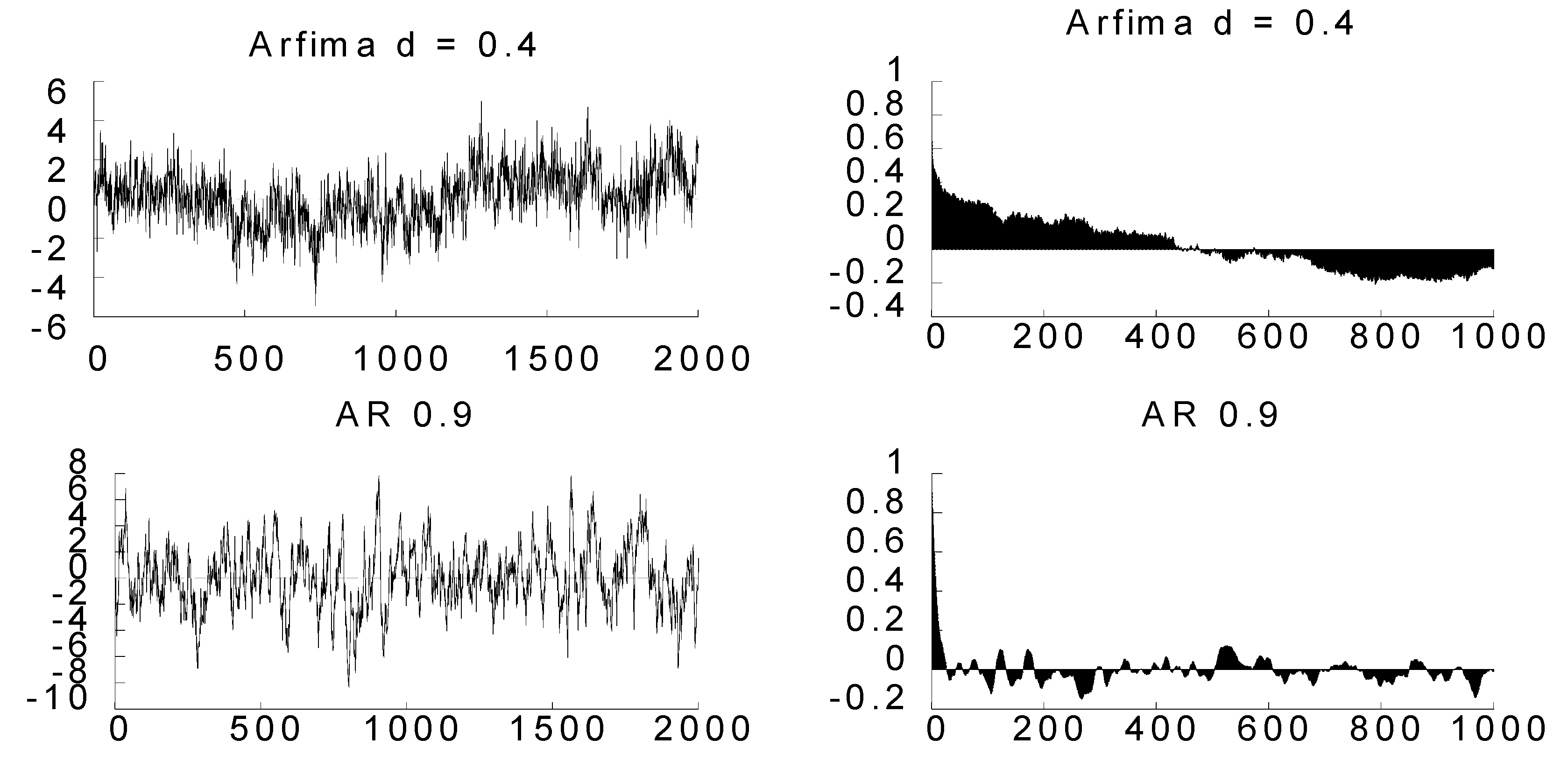
 [Green Version]
1
Geometric decay would be easily discerned in the bottom right plot in Figure 1 if the number of lags was set at most at 30 (or at any low amount).
Figure 1. Plot of Time Series. The top-left (ARFIMA d = 0.4) and bottom-left (AR 0.9) figures show the simulated series for an autoregressive fractionally integrated process with a fractional parameter d = 0.4 and an autoregressive process with a lag parameter equal to 0.9, respectively. The right-hand side shows the corresponding correlogram with 1000 lags. The correlogram shows that the autoregressive process (top right) declines geometrically to zero unlike the ARFIMA process (bottom right).
Jrfm 13 00186 g001
Figure 2. Plot of Simulated Series. The “MS Intercept” plot expresses Model 1, where the intercept switches between −5 and 1, with p11 and p12 equal to 0.99. The “MS Intercept + Autoregressive” relates to Model 2, which assumes that the model switches from a unit root to a stationary process.
Jrfm 13 00186 g002
Figure 3. Plot of Time Series. Plot of closing prices for Bitcoin, Bitcoin Cash, Ethereum, Litecoin, and XRP.
Jrfm 13 00186 g003
Table 1. Monte Carlo Simulation results. The table reports the test results of the Monte Carlo exercise. Model 1 is the model with switching intercepts (−1, 5) with probabilities of 0.95 of staying in the first regime and 0.05 from switching from the second regime to the first. Model 2 is a model which accounts for switches in both intercept (−1, −5) and autoregressive terms (1, 0.2). The models are computed using the following: Geweke and Porter-Hudak (GPH) approach with bandwidths 0.5 and 0.8, respectively, log periodogram regression with Fourier terms (as in Moulines and Soulier 1999), and the local Whittle estimator with bandwidth M = T0.5. The reported estimates are the mean over 5000 replications, and the figures in brackets report the standard deviation of the estimated parameters.
GPH (M = T0.5)GPH (M = T0.8)Fourier EstimationsLocal Whittle
Model 10.1410.5570.4670.140
(0.109)(0.026)(0.125)(0.089)
Model 20.2840.7410.4470.282
(0.147)(0.051)(0.168)(0.135)
Table 2. Summary Statistics. The table reports the summary statistics for the cryptocurrencies in the sample.
BitcoinBitcoin CashXRPLitecoinEthereum
Mean0.00102−0.00070.001490.000980.00332
Std dev0.038970.078810.072710.064440.06104
Skewness−0.3400.6122.0761.7200.271
Kurtosis8.45910.65132.9128.6187.052
Jarque–Bera2761220688925677831082
N2190882234024351553
Table 3. Long Memory Tests. The table reports the long memory test results for the five most common cryptocurrencies. Panel A exhibits the GPH estimates, bias test, and skip-sampling tests with different rates of h = 4, 8 months for returns. Panel B shows the results for three measures (i.e., proxies) of volatility: daily low high range (LHR), squared returns (SR), and absolute returns (AR). The two skip-sampling rates were chosen in favor of producing results with a narrow bandwidth. T is the sample size in number of days.
BitcoinEthereumLitecoinBitcoin CashXRP
T = 2190T = 1553T = 2435T = 883T = 2340
Estimatep-ValueEstimatep-ValueEstimatep-ValueEstimatep-ValueEstimatep-Value
Panel A: Return
GPH ( d ^ )0.1530.1650.259 **0.0360.1700.1110.1210.4050.0570.589
Bias Test−0.4540.675−1.4070.920−0.1220.5490.8060.210−0.8860.812
Skip-Sampling (h = 4)−0.5220.699−0.8160.7930.9460.172−1.0840.8610.6240.266
Skip-Sampling (h = 8)0.3780.3530.1680.4330.0440.482−0.4860.6860.5440.293
Panel B: Volatility
Volatility (LHR)
GPH ( d ^ )0.536 ***0.0000.505 ***0.0000.584 ***0.0000.541 ***0.0010.486 ***0.000
Bias Test−0.5900.7220.0440.483 *0.0840.4670.3220.3742.356 ***0.009
Skip-Sampling (h =4)−0.0730.5290.4310.333−0.7680.779−0.4510.674−0.4060.658
Skip-Sampling (h = 8)0.1930.4240.5600.288−0.4230.664−0.3070.645−0.5600.712
Volatility (SR)
GPH ( d ^ )0.326 ***0.0040.202*0.0990.359 ***0.0000.1740.2350.191 *0.077
Bias Test1.524 *0.064−1.8650.9690.3650.3573.119 ***0.0010.8680.193
Skip-Sampling (h = 4)−0.8600.8050.6370.2620.1420.4430.5850.279−0.7370.770
Skip-Sampling (h = 8)−1.0550.8540.3700.3560.5390.2950.2890.386−0.7520.774
Volatility (AR)
GPH ( d ^ )0.375 ***0.0010.378 ***0.0030.466 ***0.0000.336 **0.0260.381 ***0.001
Bias Test−2.2290.987−1.5350.9382.086 **0.0181.957 **0.025−1.1850.882
Skip-Sampling (h = 4)−1.0270.8480.4230.336−1.2290.890−0.0130.5050.0700.472
Skip-Sampling (h = 8)−1.0810.8600.8480.198−0.4820.685−0.2570.601−0.4210.663
‘***’, ‘**’, ‘*’ implies significance at the 1%, 5% and 10% respectively.

