Abstract
This paper aims to trace the monthly responses of equity prices, long-term interest rates, and exchange rates in Asian developing markets to the US unconventional monetary policy (UMP). The main research question is to explore whether UMP shocks exist in those markets. We also consider the differences in the mean responses of those asset prices between traditional and non-traditional monetary policy phases. To address such concerns, we employ a panel vector autoregression with exogenous variables (Panel VARX) model and estimate the model by the least-squares dummy variable (LSDV) estimator in three different periods spanning from 2004M2 to 2018M4. The first finding is that UMP shocks from the US are associated with a surge in equity prices, a decline in long-term interest rates, and an appreciation of currencies in Asian developing markets. In contrast, the conventional monetary policy shocks from the US seem to exert adverse effects on these recipient countries. These empirical results suggest that the policymakers in Asian developing countries should cautiously take into account the spillover effects from the US unconventional monetary policy once it is executed.
1. Introduction
The global financial crisis (GFC) has left tightened credit conditions and dysfunctional financial markets, lowering interest rates in advanced countries to the zero-lower bound (ZLB). In response to the ZLB, central banks in advanced economies engaged the unconventional monetary policy (UMP). Two types of unconventional monetary policies are, first, a forward guidance of future interest rates, and second, large-scale asset purchases (LSAPs)1, which refers to purchasing a large amount of both Treasury and agency securities2. Particularly, on November 2008, the US Federal Reserve initiated ‘quantitative easing’ (QE) by which a central bank purchases government securities, aiming at altering the global conditions (Rafiq 2015) and providing liquidity to ailing financial sectors (Wright 2012). During five years of policy implementation, the balance sheet of the Federal Reserve enlarged more than five-fold, reaching $4.5 trillion in 2014 (Wolfers 2014). Moreover, the UMP also impacts internationally upon other nations. Brana et al. (2012) suggest that excess global liquidity is able to boost the economic prospect in developing nations. On the other hand, Lorenzoni (2008) argues that large capital inflows can result in a credit boom, thus leading to a collapse in asset price and further causing economic and financial instability in the recipient countries. Tillmann (2015) refers to the argument of Brazil’s President Dilma Rousseff to describe QE shocks as ‘sudden floods’ of liquidity to hit developing and emerging countries, which might lead to severe consequences on economic fundamentals of one country. Specifically, it is widely known that Asian countries have become more integrated into the global market and especially the US economy. Therefore, the spillover effect of UMP is predicted to occur in the Asian economies (Xu and La 2019). International capital flows could bring harmful consequences for the developing countries (Brana et al. 2012). Kawai (2015) emphasizes that policy makers in these countries should deeply understand the spillover effect to establish corresponding policies. However, while most of the literature tends to focus on large emerging nations (Bhattarai et al. 2018; Tillmann 2015), less research focuses comprehensively only on Asian developing countries, which includes both emerging and frontier markets. Park et al. (2013) argue that global instability is likely to substantially threaten the growth and prospect of Asian nations. Particularly, Southeast Asian nations also have a long history of economic ties with the US, which is the dominant player in trading. After the GFC, Indonesia and the Philippines witnessed fragile economies, awkward policies, and a great loss of investor confidence. Of all nations, China experienced the largest equity outflows from the US after several rounds of QE programs (Khatiwada 2017). Thus, investigating the macro-financial risks facing the developing countries in Asia against the shocks from unconventional monetary policy in the US is strongly needed. On top of that, understanding how unconventional monetary policy affects these economies plays an important role, which could later provide precise guidance for policymakers.
This study is mainly motivated by the work of Bhattarai et al. (2018) and Punzi and Chantapacdepong (2019), in terms of the measurement of UMP shock and econometrics used. Bhattarai et al. (2018) adopt a Vector Autoregressive (VAR) model to identify the US QE shock and then employ a monthly Bayesian panel VAR to examine the spillover effect of this shock on emerging countries. In a sensitivity analysis, the authors use the shadow short rate to gauge US QE. Punzi and Chantapacdepong (2019) also proxy the US UMP shock by using the shadow short rates proposed by Krippner (2013). The authors employ a Panel Vector Autoregression model to examine the spillover effect from the US to Asia and the Pacific region, showing an increase in asset prices and currency appreciation in the recipient countries.
In general, our study extends the literature in four areas. First, to the best of our knowledge, this is the first study that comprehensively addresses the change of three different asset prices in the group of Asian developing markets, which are equity prices, long-term rates, and exchange rates, in pre-UMP, during UMP, and post-UMP phases. We would provide additional evidence on the spillover effect from the US UMP to other developing countries in Asia for instance, Vietnam, as such previous work is still limited. Arguably, the previous research into Asian markets focuses only on bank lending channels, such as that of Xu and La (2019). Other research considers the means of linking to a broad set of nations including Asian and Latin American markets. Most research neglects asking whether UMP shocks will exert net negative or positive influences on Asian nations. Second, our study compares the impacts of unconventional and conventional monetary policies from the US on these countries by investigating three asset prices’ mean responses, in terms of the size and significance. Third, our paper employs a methodological approach named panel VARX (panel vector autoregression with exogenous variables), which is rarely formulated by previous work in studying the spillover effect of the US unconventional monetary policy on the Asian developing nations. This method allows to pool the experiences of different countries from time to time to derive the mean responses of three asset prices in Asian developing countries. Fourth, this study also traces the mean responses of asset price to the monetary policy shocks in every month of and after the event.
In light of these concerns, to explore such potential challenges, this research would focus on the impact of the expansion of monetary aggregates in the US on asset prices in Asian developing markets. This study also investigates the channels through which UMP shocks will affect financial and macroeconomic conditions in Asian developing countries. Two main questions are addressed in this paper:
- Once the US unconventional monetary policy is enacted, does it spill over into Asian developing countries? Particularly, how does UMP from the US impact on different asset prices, including equity prices, long-term interest rates, and exchange rates in Asian developing markets? How large and pervasive are the effects?
- Is there any difference in the mean responses of asset prices in Asian developing countries between unconventional and conventional periods?
2. Theoretical Framework
Generally, the model that is widely adopted in studies of external monetary policy shocks is the Mundell–Fleming (MF) model initiated by Mundell (1963) and Fleming (1962), which is adapted from the investment saving–liquidity preference money (IS–LM) supply model. Frenkel and Razin (1987) firstly apply the Mundell–Fleming model to study the transmission of monetary shocks between nations. Specifically, according to this model, an expansionary monetary policy would depreciate the value of the currency in the home nation and deteriorate its terms of trade, thus leaving cheaper home goods for foreign nations. Thus, such depreciation would be accompanied by a decline in output volume in the foreign countrie3. Dornbusch (1976) extends the Mundell–Fleming model to indicate that loosening the monetary policy would more greatly impact upon asset prices in the long run. Notably, this type of policy is currently expected to raise the expectation of money supply, hence affecting asset price volatility. Thus far, an updated version, namely, the Mundell–Fleming–Dornbusch model, was then introduced. In short, this theory framework refers to the exchange rate channel through which an expansionary monetary policy in one country would lower interest rates and appreciate local currencies in the partner countries.
Using the Mundell–Fleming (MF) model initiated by Mundell (1963) and Fleming (1962), Joyce et al. (2011) comprehensively study five transmission channels: money, policy signaling, portfolio rebalancing, market liquidity, and confidence effects (as seen in Figure 1). Within these, the three main channels of UMP transmission are portfolio rebalancing, signaling, and liquidity channels (Neely 2015). What follows details how each channel operates?
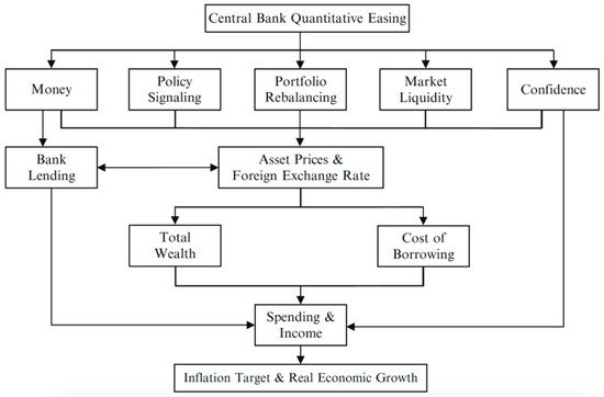
Figure 1.
Transmission channels of quantitative easing (adopted from Joyce et al. (2011)).
Concerning the portfolio balance channel, it is crucial to comprehend the ‘preferred habitat theory’ for investors, which has significantly influenced the yields of securities being purchased and their close substitutes. Generally, investors would place their capital in long-term safe investments (Krishnamurthy and Vissing-Jorgensen 2011). However, once the Federal Reserve purchases securities, the portfolio rebalancing channel will produce its effect so that the amount of assets held by private sectors reduces. Therefore, they are inclined to invest in international securities that closely substitute for US assets being purchased (Hausman and Wongswan 2011). Consequently, this purchase program bids up the price of the assets being bought under the LSAPs as well as their substitutes, thus lowering yields and the term premium of these assets until the new equilibrium is reached.
Regarding the signaling channel, the announcements of non-traditional expansionary monetary policy aim to signal that the future course of short-term interest rates will continue to decline. By implementing LSAPs, the Federal Reserve aims to sustain an expansionary monetary policy for a longer time than expected previously. The signaling effect refers to the perceptions of central banks about future economic conditions. For example, an expectation of worse conditions will increase the demand for T-bills from investors, and such a signal will immediately lower the average, expected short-term yield, which is a crucial component of a bond yield over longer terms.
As for the liquidity channel, the greater participation of the central bank in the market is expected to increase market functioning and also reduce the liquidity premium required (Joyce et al. 2011). Furthermore, an increasing liquidity flow following QE policy would help boost equity and property prices. Through this channel, the QE policy is expected to stimulate more investments in riskier assets. Consequently, by boosting wealth and the level of spending, the expansionary policy will significantly contribute to greater consumption, production, and employment.
Other channels also mentioned by Joyce et al. (2011) were the confidence and bank lending effects. Once the economic outlook improves, market participants will be more confident purchasing assets, resulting in increased prices and declined risk premiums. Relevant to the bank lending channel, UMP policy would benefit the banking sector by increasing the broad money held by people after they purchase large assets.
Generally, these transmission channels indicate that UMP shocks will cause interest rates to decline and stock prices to increase. Adding to this, commodity prices tend to decline in response to the announcements of LSAPs. Nevertheless, according to Glick and Leduc (2012), LSAPs could also raise the security yields and commodity prices given future expectations of lower risk.
Another theoretical model has been proposed in a recent study by Alpanda and Kabaca (2020), which is named “the two-country dynamic stochastic general equilibrium model”. The authors employ this model with nominal and real rigidities, as well as a portfolio balance effect to explore the domestic and international spillover effect of US QE round 2. Alpanda and Kabaca (2020) point out that the inadequate substitution between short- and long-term government bonds or between domestic and international and foreign bonds leads to the portfolio balance effect among countries. In other words, as these kinds of bonds cannot perfectly substitute for each other, a decrease in supply will result in a drop in long-term rates. Such a fall in long-term rates in one country will then create pressure for a nominal appreciation of local currencies in other economies and stimulate the demand for foreign assets. Alpanda and Kabaca (2020) also emphasize the stronger effect of portfolio balance under the implementation of unconventional monetary policy.
All in all, the theoretical points of view have not delivered clear-cut arguments on whether a loosening monetary policy in a home country can exert positive or negative effects on recipient countries. Indeed, the final conclusion is determined by the relative strength of each channel, which awaits much empirical studies.
3. Literature Review
Generally, there exists two strands of the literature on this topic. The first explores the determinants of shocks to developing countries (Fratzscher 2012). Second are studies investigating the impact of unconventional monetary policy shock on real and financial variables in emerging markets (Bowman et al. 2015). Concerning the measurement of the Fed’s policy stance applied after the GFC, earlier studies used two primary categories of analysis, namely event study and balance sheets’ assets changes.
Event studies generally follow two research courses: first, the announcements of the Federal Open Market Committee (FOMC) meetings and speeches by Chairman Bernanke; and second, they assess changes in the term structure of interest rates. The most popular approach to event study analysis used in the literature is to investigate the impact of monetary policy shocks on asset prices through the signaling and portfolio balance channels (Gagnon et al. 2011; Hancock and Passmore 2011; Krishnamurthy and Vissing-Jorgensen 2011; Doh 2010; Hamilton and Wu 2012).
Much research uses event-study analysis, starting with Gagnon et al. (2011), followed by Krishnamurthy and Vissing-Jorgensen (2011), and Wright (2012) and Neely (2015). Some focus on the domestic financial markets (Gagnon et al. 2011; Glick and Leduc 2012), while some also consider international financial markets (Hausman and Wongswan 2011; Neely 2015). However, less research investigates the impact of non-standard policy shocks on the real economy, as Dahlhaus et al. (2018) do. The high-frequency event-study analysis of Wright (2012) considers the total effect of monetary policy shocks on intraday changes of asset prices. Such analyses point to a negative relation between three QE periods and the interest rates that are reserved over the following periods. In a model-based event study, Bauer and Rudebusch (2014) suggest that around 30% to 65% of the total impact on term structure is attributable to the signaling effect, while Gagnon et al. (2011) document that this channel only accounts for 30% of the changes in interest rates. Bauer and Neely (2014) measure three rounds of asset purchases including QE1, QE2, and QE34 by estimating the importance of signaling and portfolio balance channels with the focus on the term structure of interest rates.
Likewise, following a standard event study, Hausman and Wongswan (2011) find that nations with rigid exchange rate regimes would have a greater reaction in the equity market and a larger interest-rate response. Hancock and Passmore (2011) find that monetary surprises create substantial downward pressure on mortgage rates through the portfolio rebalancing channel. Christensen and Rudebusch (2012) use monthly international excess bond returns to estimate the impact of QE surprises from the US on other developed nations. They document a positive covariance between the US and Australian long bond returns, signifying that the portfolio balance effect is dominant in this market rather than signaling channel. Hancock and Passmore (2011) find that QE surprises create substantial downward pressure on mortgage rates through the portfolio rebalancing channel. This channel specifically explains half the decline in mortgage rates after the statements released by the Federal Reserve. Although the magnitude of the QE2 surprise was greater than that of QE1, Glick and Leduc (2012) surprisingly show a greater daily movement in long-term interest rates on days of LSAP1 announcements. Aizenman et al. (2016) conduct a ‘quasi-event’ and show that a country characterized by a strong fundamental will respond more to the tapering statements compared to a weak country.
Concerning the second measurement of policy stance, the central bank balance sheet, researchers used to base their approach on the changes of components on the balance sheet as per unconventional monetary policy. Bhattarai et al. (2018) argue that securities held outright are the main components of QE policy in the US, especially after ZLB started binding. Bhattarai et al. (2018) also evidence a stronger impact of QE shocks on financial variables compared to that on real macroeconomic variables. Additionally, Dahlhaus et al. (2018) proxy the unconventional monetary stance by the long-term assets on the US Federal Reserve’s balance sheet. From studying the spillover effect of QE programs on the East Asian market, Morgan (2011) defines the stance of policy based on the outright purchases of US Treasury notes and bonds. After comparing the statistics, he concludes that QE programs only slightly impact upon these markets.
Anaya et al. (2017) also identify the UMP shocks through changes in the balance sheet of the Fed by focusing on the role of financial flows. Additionally, the unconventional monetary policy shock from the US is associated with an increase in equity return, an appreciation in currencies, and a decline in the real lending interest rate in emerging economies. This confirms the previous studies related to the impact of UMP shocks on asset prices in foreign countries. Anaya et al. (2017) also consider the economic characteristics, the degree of financial openness to global markets, and the institutions of emerging countries to explore the heterogeneous effects of UMP shocks. Their results show less evidence of heterogeneity among recipient countries in response to the excess liquidity spawned from the US.
MacDonald (2017) measures the policy stance of the Fed during the aftermath period by five different types of assets in balance sheets with the gravity-in-international-finance model, indicating significant differences in the responses of emerging market economies (EMEs) to the monetary shocks from the US. MacDonald (2017) eventually points to a salient suggestion, recommending policymakers in emerging countries to orientate their monetary policies earlier by cautiously bearing in mind the level of market friction and trade integration in the global market earlier.
In the same vein, Matousek et al. (2019) gauge the quantitative easing shock from the Bank of Japan as the current account balance changes. With a focus on the bank lending channel, the authors explore the effect of quantitative easing conducted by the Bank of Japan on the assets and liabilities composition of regional banks by applying a Panel VAR. The main finding signifies an increase in the degree of leverage for small banks with high non-performing loans under the QE shock, boosting the ability of these banks to take higher risks. Furthermore, QE shock in Japan seems to exert a positive and long-lasting effect on macroeconomic variables, including GDP and inflation.
Fratzscher et al. (2018) provide two reasons for measuring policy stance based on the actual asset purchased rather than on FOMC announcements. First, asset purchases could capture the liquidity of actual market operations by the Federal Reserve during the aftermath. Second, it is inaccurate to measure the effectiveness of non-standard monetary policy by market expectations following the announcements (Fratzscher et al. 2018).
Regarding the econometric method, most studies adopt the VAR model or related methods including panel, global, Bayesian, and factor augmented vector autoregressive models (Gambacorta et al. 2014; Punzi and Chantapacdepong 2019; Bhattarai et al. 2018) to examine the UMP shocks. Using a Panel VAR, Punzi and Chantapacdepong (2019) indicate that central banks in Asia and the Pacific regions respond by lowering policy rates to allay further appreciation. The responses of central banks in these regions show that central banks are gradually losing their independence to decide their monetary policy stances. Inoue and Rossi (2019) advise a new approach by applying ‘VARs with functional shocks’. Similar to the previous work of Wright (2012), Inoue and Rossi (2019) observe the impact of news on the yield curve to gauge UMP. However, while monetary shocks are usually measured by the exogenous changes in short-term interest rates in previous work, Inoue and Rossi (2019) differently measure the economic shocks as functional rather than scalar. In other words, these authors consider the shift of the yield curve and how key macroeconomic variables respond to the joint change of the curve. The empirical results point to an increase in output and inflation in the US with a peak after one year.
Employing the Panel VAR model, Punzi and Chantapacdepong (2019) also indicate that central banks in Asia and the Pacific regions respond by lowering policy rates to allay further appreciation. The responses of central banks in these regions show that central banks are gradually losing their independence to decide their monetary policy stances. Pham and Nguyen (2019) evaluate the spillover effect of UMP from the US on the monetary policies in Asian countries by a Bayesian vector autoregressive model. To address such an issue, this research considers how policy rates in Asian countries respond to the shock to the Fed policy rate. The empirical results indicate a co-movement between policy rates in Asian economies and the US with a lag of one quarter. Concerning the size of responses, Asian developing countries characterized by pegged rate regimes significantly respond to innovations in the Fed rate, while the developed ones are less likely to be affected by the UMP shocks.
Nevertheless, there are still considerable gaps in the literature. Few studies either compare the different impacts between conventional and unconventional monetary policies or indicate whether the impact of financial variables outweighs that of macroeconomic variables. As far as we are concerned, only Bhattarai et al. (2018) take account of this matter. In addition, there is no consensus on which is the most appropriate measure of policy stances of the US Federal Reserve during the aftermath. While event studies cannot reflect the impacts of monetary surprises on macroeconomic variables, the changes on a central bank balance sheet also fail to comprehensively capture policies related to non-standard policies—for example, the forward guidance (Macdonald and Popiel 2017). Notably, little research addresses the spillover effect of UMP on both macroeconomic and financial conditions in Asian developing markets. For instance, Miyajima et al. (2014) only focus on the direct role of the interest rate channel but do not investigate in other channels such as portfolio rebalancing or market liquidity channels. Cho and Rhee (2014) investigate how the US monetary policy influences the capital inflows and financial condition in Asia. Nonetheless, Cho and Rhee (2014) do not address how stock markets in Asia are influenced by monetary surprises and do not account for the potential spill-over effect of UMP from the US.
After noting these gaps and varying empirical results, we aim to study the spillover effect of the UMP from the US on Asian developing nations to an extent that could complement previous studies. To the best of our knowledge, this is one of the first studies that focuses on this group of recipient countries considering the changes of different asset prices. Different from previous research in Asian countries, we measure the policy stance based on the shadow short rate (SSR), as it can capture the overall policy stance that comprise LSAPs and forward guidance by the Fed. Although Neely (2015) uses event-study analysis, he nonetheless argues that including a set of suitable events is not easy to achieve. Specifically, researchers would exhibit bias if they excluded events that are associated with changes in LSAP expectations. Applying extraneous events to model-based event studies is also inefficient. Lombardi and Zhu (2018) also relate the shadow short rate to a close approximation for monetary surprises once the zero lower bound is binding. On top of that, the shadow short rate is in line with Taylor rules. With these distinctions, we aim to contribute meaningfully to the literature.
4. Data and Methodology
4.1. Data
The sample contains 8 Asian developing countries according to Morgan Stanley Capital International (MSCI) classifications: China, India, Indonesia, Malaysia, South Korea, Thailand, the Philippines, and Vietnam5. The monthly data cover the period from February 2004 to April 2018 with the primary sources being the Bloomberg and International Monetary Funds (IMF) databases. As the real GDP is not available at a monthly frequency, we employ the Chow–Lin procedure for temporal disaggregation. The US data were retrieved from Federal Reserve Economic Data (FRED). In this research, we engage the SSR by Krippner (2013) to measure monetary policy in the US, as it provides an explicit function to inspect the shadow rate curve (Lombardi and Zhu 2018).
The idea of using the shadow rate term structure model was initiated by Black (1995), accounting for the ZLB period. As can be seen from Figure 2, the shadow short rate can be positive or negative. If the shadow short-term rate is above the lower bound, it is equal to the observed short-term rate. Hence, these two rates are not equivalent when the short rate effectively hits the ZLB or QE is enacted. The one-period SSR is specified by a term structure model, as follows:
Upon this point, a surprise in SSR is regarded as an UMP shock once the non-traditional policy is effective; otherwise, it is just a conventional monetary policy shock.
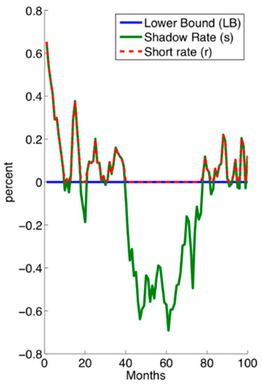
Figure 2.
Short rate and shadow rate association (adopted from Lemke and Vladu 2017).
Doh and Choi (2016) argue that the 10-year interest rate could be a proper proxy of unconventional monetary policy during the ZLB period as it reflects the current and future short-term interest rate. From this idea, they suggest constructing a shadow short-term interest rate as a good candidate for unconventional monetary shock. Krippner (2013) and Wu and Xia (2016) both postulate that the SSR is a more accurate measure of policy stance rather than the fund rate itself, as the SSR is likely to diverge from the short-term rate given a ZLB constraint. In short, the SSR closely tracks the funds rate executed by the US Federal Reserve since the onset of ZLB.
A variety of research methods can estimate the US SSR. Wu and Xia (2016) estimate the SSR with the latent factor based on a panel of monetary and financial quantities. Krippner (2016) uses an option-based approach to obtain the shadow rate. The SSR used in this research was adopted from the measure of Krippner (2016), which incorporated two latent factors. Damjanović and Masten (2016) suggest that, compared to that of Wu and Xia (2016), the estimate of Krippner (2016) is a superior proxy for policy stance. Wu and Xia (2016) also identify another advantage using Krippner’s measure: to maintain the stability of the parameters and deliver favorable robustness checks of the choice of the sample period.
Table 1 depicts the data statistics in this research. Other details are presented in Appendix A. We use monthly data for three samples spanning 2004M2–2007M12 (pre-UMP period), 2008M9–2014M1 (during the UMP period), and 2014M2–2018M4 (post-UMP period) and focus on 8 Asian developing economies. The rationale is to exclude the period when the market witnessed abnormal volatility, which might lead to biased results. Additionally, to answer the second research question of examining the differences between conventional and unconventional monetary policies in the US, we split out the second phase 2008M9–2014M1 as the UMP period, corresponding to the period when QE1, QE2, and QE3 are sequentially executed. In other words, any surprise within 2004M2–2007M12 or 2014M2–2018M4 is considered as a conventional monetary policy shock, also referring to MP shock later on in this paper.

Table 1.
Descriptive Statistics of Panel Data for Three Periods. UMP: unconventional monetary policy.
As mentioned earlier, we study the impact of UMP shocks on three different asset prices in Asian economies, which are equity prices, long-term interest rates, and exchange rates. The variation of three asset prices is presented in Figure 3, Figure 4 and Figure 5 accordingly. GDP growth and inflation are included as the control variables for domestic macroeconomic conditions.
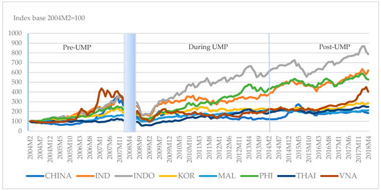
Figure 3.
Equity prices in Asian developing countries for the whole period (source: Bloomberg). CHINA = China; IND = India; INDO = Indonesia; KOR = Korea; MAL = Malaysia; PHI = Philippines; THAI = Thailand; VNA = Vietnam.  Crisis period.
Crisis period.
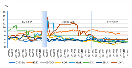
Figure 4.
Long-term interest rates in Asian developing countries for the whole period (source: Bloomberg, national sources). CHINA = China; IND = India; INDO = Indonesia; KOR = Korea; MAL = Malaysia; PHI = Philippines; THAI = Thailand; VNA = Vietnam.  Crisis period.
Crisis period.
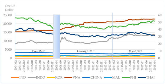
Figure 5.
Exchange rates in Asian developing countries for the whole period (source: Bloomberg). CHINA = China; IND = India; INDO = Indonesia; KOR = Korea; MAL = Malaysia; PHI = Philippines; THAI = Thailand; VNA = Vietnam.  Crisis period.
Crisis period.
As can be seen from Figure 3, it is likely that there is an upward trend in equity prices after 2008M9 when the US launches its first quantitative easing program. Figure 4 visually shows more volatile interest rates in Asian developing countries when the UMP from the US is implemented, except for the Philippines. Figure 5 describes the variation of local currencies in Asian developing countries versus the US dollar, in which the second axis is for China, Malaysia, Thailand, and the Philippines. It seems that there is a declining trend of exchange rates during the UMP period in Asian developing countries, implying an appreciation of local currencies.
4.2. Econometric Methodology
The research will be implemented in two steps:
- Identifying shocks from unconventional monetary policy.
- Tracing out the spillover effects of unconventional monetary policy in the US on Asian developing countries.
4.2.1. Identifying Shocks from Unconventional Monetary Policy
Structural Vector Autoregressive Model
Generally, the monetary shocks can be identified by two main approaches. The first method is to gather evidence from the course of historical events. Friedman and Schwartz (2008) initiated the idea of tracing out the changes in monetary aggregates during a 10-year period. Similar to this vein, by employing this narrative record, Romer and Romer (2004) indicate that the Fed’s monetary policy significantly affected inflation and growth in the US. Nonetheless, Lombardi and Zhu (2018) point to the endogeneity of policy intentions that might merge with other shocks. In other words, when the monetary policy reacts to the effect of other macroeconomic variables, it is difficult to measure the pure impact of the policy on the economy. Second, vector autoregressive (VAR) models have been widely employed in previous work to investigate the variation of monetary policy. Early VAR studies on this topic are conducted by Bernanke and Blinder (1992) and Christiano et al. (1996). However, Rudebusch (1998) argues that the VAR model fails to distinguish between exogenous and endogenous monetary policy actions, resulting in bias covariance matrix. Moreover, the recursive form of VAR could not capture the simultaneous interactions between variables. Thus, the recursive VAR approach leads to misinforming inferences regarding the impact of monetary surprises on macroeconomic variables (Bhuiyan 2012). Specifically, Stock and Watson (2001) emphasize that structural VAR (SVAR) has the remarkable ability of identifying the causal links in the model, allowing simultaneous interactions among variables. SVAR is typically preferred to VAR for analyzing economic shocks, since VAR serves mainly to forecast. Then, structural VAR (SVAR) is suggested as a useful tool to analyze the economic shocks stemming from policy interventions and changes in policy conditions, especially monetary policies. Sims and Zha (2006) also add to the literature by imposing more structure on the VAR to investigate the endogenous features of monetary policy. Kim and Roubini (2000) also employ the SVAR approach in their research of the US QE shocks on G7 countries, clarifying the liquidity puzzle, price puzzle, and exchange rate puzzle. Their methodology is in the same vein with Sims and Zha (2006), using non-recursive identification restrictions upon economic theories. In association with previous studies, the authors also find that the non-traditional monetary shocks from the US significantly affect the output level of other economies in G7 members.
All in all, identifying only the exogenous shocks would help to ascertain the dynamic effects of the unconventional monetary policy. Hence, applying a structural VAR model is much needed in this case.
Sims (1980) signifies that SVAR is one of the most practical classes of models for empirical macroeconomics and finance. Furthermore, the advantage of SVAR is to predict the impacts of intervention of public policies, especially monetary policy (Sims 1980). Since SVAR allows greater flexibility in economic content, it has been widely adopted as a useful means of analyzing the macroeconomic effects of both traditional and non-traditional monetary shocks. By employing the SVAR approach, Lombardi and Zhu (2018) also document that the monetary policy shocks could better explain the UMP stance of the Federal Reserve. As we intend to delay the transmission of monetary policy, its effects should be restricted. To impose such restrictions, structural VAR is thus the most suitable approach in this research. Regarding the US economy, we use a SVAR model as follows:
in which is a vector of endogenous variables, which will be later detailed later in this paper. In addition, follows the normal distribution . Moreover, E (.
In this model, we assume that the structural shocks are orthogonal and can thus ascertain the relationship between the errors of the reduced and structural forms, as follows:
Breitung et al. (2004) explain the setting of linear restrictions of A and B matrices, and they specify the additional restrictions needed for identification:. Therefore, the system becomes exactly identified. It is important to note that a proper identified structural model would help lessen the probability of endogeneity problems.
Kim (2001) is one of the first to approach SVAR to estimate the QE shocks from the US to other nations. The author uses the SVAR model by setting up both recursive and non-recursive contemporaneous identification restrictions and found similar results under these two schemes. The study finds that unconventional monetary policy from the US impacted positively upon the output of non-US G6 economies. Similarly, Bhattarai et al. (2018) and Bacchiocchi et al. (2017) obtain consistent results when using either a non-recursive or recursive structure on a standard SVAR to identify the US monetary shocks. The intuition behind the model is that macroeconomic variables respond with a delay to monetary shocks (Bacchiocchi et al. 2017). In addition, monetary variables are assumed to respond immediately to the shocks of ‘slow-moving variables’ (Bacchiocchi et al. 2017). Therefore, in this study, we impose the recursive structure on the contemporaneous relationships among variables to identify the shocks.
Benchmark Identification of Structural Shock
The focus of this research is to identify and measure monetary shocks that cause foreign financial markets to react. This research employs a theory-based restrictions SVAR approach to identify monetary policy shocks when the economy gets stuck at ZLB. The identification of structural shocks in this model will use exact restrictions, based on the beliefs of the relationship between variables. Imposing additional zero restrictions would help to reduce the number of admissible impulse responses. Thus, the identification would be sharpened, given that zero constraints are realistic. The focus is still on capturing the UMP structural shocks. The AB model adopted in this analysis was introduced by Amisano and Giannini (1997).
Generally, as the MP shocks can be understood as an unanticipated deviation from the monetary policy, this deviation is exogenous to the US macroeconomic condition. Macdonald and Popiel (2017) adopt an upper triangular matrix with the order {policy rate, VIX index, commodity export price, price, output} to identify the unconventional monetary policy shocks. Gambacorta et al. (2014) assume that stock market volatility would not respond to the UMP shocks. Output and prices would not be expected to react to the changes of monetary policy within a month, according to Leeper et al. (1996) and Macdonald and Popiel (2017). Gambacorta et al. (2014) also assert that monetary shocks only affect macroeconomic variables with lags. In other words, because the growth rate and price level would not change in the short term, the contemporaneous impacts of MP shocks on these variables are restrained to zero.
This research thereby follows Macdonald and Popiel (2017) in ordering the variables. Table 2 summarizes the restrictions considered for the benchmark model, as follows. The first series of structural shocks is obtained as SSR shocks, in which data spanning within 2008M9–2014M1 are UMP shock. The structural shocks in other periods refer to MP shocks during the conventional monetary policy of the US.
Table 2.
Identifying restrictions-benchmark identification.
An alternative identification of UMP shock is employing a mixture of zero and sign restrictions on the contemporaneous impact matrix B in Equation (2). This kind of combination has been widely used in earlier studies to identify structural shocks (Gambacorta et al. 2014; Eickmeier and Hofmann 2013). For example, Gambacorta et al. (2014) impose zero restrictions on the mean responses of macroeconomic variables including output and price level to disentangle the real economy from the monetary shocks. The sign restrictions are used for the VIX, as unconventional monetary policies will lessen the risk in the stock market (Gambacorta et al. 2014).
Additionally, the specification can be extended by adding or replacing one or two variables to the baseline model at a time, as done by Bhattarai et al. (2018). For instance, in identifying the QE shocks, these authors add house prices and corporate bond yields to the baseline specification. In addition, they replace industrial production by monthly GDP as an alternative identification.
4.2.2. Tracing Out the International Effect of Non-Standard Monetary Policy from the US on Asian Developing Countries
Previous research regarding the spillover effect of UMP policy on Asian markets usually adopted a normal Panel Analysis or Panel VAR to address the issue such as Brana et al. (2012) and Bhattarai et al. (2018). The Panel VAR was introduced by Holtz-Eakin et al. (1988), which is considered as a pair of extensions based on panel data analysis and VAR. The most important assumption of Panel VAR is that the slope coefficients for all individuals are identical. Pedroni (2013) emphasizes the advantage of this method of suitability for unbalanced panels, allowing researchers to process the panel data with different timespans among individuals. Specifically, as monetary policy shock from the US is exogenous to the economic condition in Asian developing countries, we adopt a Panel VARX, which means a Panel VAR with exogenous variables. The economic model is expressed as follows:
The sample includes 8 countries, which are indexed as i = 1, 2, 3, … N, and the time index for country i is t = −1, 0, 1, …, Ti; and represent individual effects and idiosyncratic error terms in the system; while p and q are the lag lengths of endogenous and exogenous variables, respectively. Belke et al. (2010) suggest placing macroeconomic variables before financial variables, implying that output and inflation should be placed before asset prices. Hence, the 3 × 1 vector of endogenous variables comprises real output growth, inflation, and one of three asset prices in Asian developing countries, which is detailed as below:
One exogenous variable is the monetary policy shocks retrieved from the SVAR model, which is common to all countries in our sample. We assume that , for all i and t. Additionally, we assume that within equations, the errors are independent with s t. This assumption is also set across equations, for for any s and t where i j.
Once a country’s fixed effects are controlled, Equation (3) can be compactly inverted as follows:
where L represents the usual lag operator. The mean responses of asset prices to monetary policy shocks can be obtained by the lag polynomial:
We adopt the least-squares dummy variable (LSDV) in simulations to the Panel VARX model with an unbalanced panel based on the following rationale. According to Fomby et al. (2013), the LSDV method yields good estimates, as bootstrap bias-corrected estimator does, given the annual data for a period of 35 years for each country. Thus, the LSDV method is also likely to suit our monthly panel data in each of the three phases. Although Nickell (1981) emphasizes the inconsistency of an LSDV given a dynamic model with small T, this problem can be corrected as T grows (Cavallari and D’Addona 2015). Concerning our sample, the time dimension characterized by the monthly panel data is relatively large enough for the LSDV estimator.
4.3. Diagnostic Tests
4.3.1. Panel Unit Root Tests
It is essential to consider the properties of data in time series analysis, the purpose being to ensure that the methodology is appropriate and the conclusions are accurate and reliable. Accordingly, in this research, we conduct the panel-unit root tests for the stationary properties of the variables included. The variables of interest are: (1) real GDP growth; (2) inflation; (3) equity prices; (4) long-term interest rates; (5) exchange rates and (6) monetary policy shocks retrieved from the SVAR model of the US economy.
We use the panel unit root test developed by Breitung (2000), which is able to adjust the data before employing them to the regression model. The null hypothesis is that all the time series in the panel dataset contain a unit root, versus the alternative hypothesis that each individual in the panel does not have a unit root. Additionally, the Breitung procedure exhibits a higher statistical power when the panel-specified effects are presented in the regression model or autoregressive parameters close to one, compared to the Levin–Lin–Chu7 test. The basic Augmented Dickey–Fuller specification considered in the Breitung test is specified as:
In the Breitung test, the null hypothesis denotes that all have a unit root:
Then, the alternative hypothesis is expressed as:
Another unit-root test procedure performed in this research is that of Im et al. (2003) (Im – Pesaron–Shin, IPS), which is more powerful than the Levin–Lin–Chu test (Maddala and Wu 2001). Im et al. (2003) propose the panel unit root test under the assumption that not all the same autoregressive parameters are identical. The most significant advantage of IPS’s test is that it accounts for cross-sectional dependence by involving cross-sectionally Augmented Dickey–Fuller for each cross-sectional unit (Herzer and Vollmer 2012). For the IPS’s test, the alternative hypothesis is:
4.3.2. Lag Structure
Before estimating the SVAR model for the US economy, it is important to select the lag structure. Two well-known criteria are engaged: Akaike’s information criterion (AIC) and Schwarz’s Bayesian information criterion (SBC). According to Fomby et al. (2013), the higher the lag lengths, the more informative the impulse response function (IRF).
Additionally, the appropriate lag length is crucial before estimating the panel VARX. If a too-short lag length is used, the dynamics of the systems cannot be properly captured, and bias problems will occur with the omitted variables issue. On another hand, too many lags cause a loss of the degree of freedom in the model, resulting in the over-parameterization problem. The optimal lag length can be chosen based on the moment and model selection criteria (MMSC) introduced by Andrews and Lu (2001). They proposed three criteria: modified Bayesian information criterion (MBIC), modified Akaike information criterion (MAIC), and modified Hannan–Quinn information criterion (MHQIC), which are similar to the common model selection criteria, namely the BIC, AIC and HQIC. The estimators proposed by Andrews and Lu (2001) are presented as follows:
in which p and q are the lag lengths of endogenous and exogenous variables, respectively. The order that has the smallest values of MAIC, MBIC, and MHQIC will be selected.
5. Results
5.1. Benchmark Results of Structural Shock
Then, the SVAR estimation proceeds with the constraints introduced previously. The optimal lag selected by AIC is 2, while SBC criterion suggest the lag of 1. We select the lag length of 2 for the SVAR model, based on AIC criterion.
The IRFs of US macroeconomic variables to one standard deviation of SSR shocks is depicted in Figure 6 above. As commonly evidenced in previous studies (Anaya et al. 2017; Gambacorta et al. 2014), unconventional monetary policy exerts a positive shock on real GDP growth, which peaks at around 0.04%. This finding is in line with the visual inspection data earlier, implying that the expansionary monetary policy in the US during the aftermath helps boost economic growth in this country. Likewise, the response of inflation on the Fed’s enlargement of balance sheet is positive. The response of price level reaches its peak of 0.05% and lasts up to 5 months. Figure 6 also indicates a negative response of VIX Index to monetary policy shocks after 2 months, which is analogous to Gambacorta et al. (2014). As a prime gauge of stock market volatility, a negative response of VIX Index implies that the monetary policy mitigates the fear of financial turmoil and economic instability in the US. As expected, after loosening the monetary policy, the long-term interest rate gradually decreases, indicating market participants’ expectation of a lower interest rate. Afterwards, the first series of structural shocks is then retrieved as the measure of monetary policy shocks for subsequent analysis in the international context in Section 5.2.
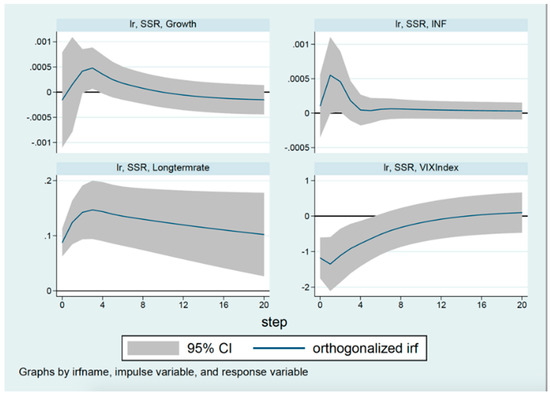
Figure 6.
Impulses responses of US macroeconomic variables to monetary policy shocks.
5.2. Panel VARX Estimations
As mentioned previously, this paper aims to figure out whether the UMP from the US influences three asset prices in Asian developing countries. Specifically, we would also investigate the direction of UMP effects in comparison with MP effects. To address such an issue, we include one asset price at a time in Equation (4). Upon MBIC criterion, a lag length of one is selected for three periods: pre-UMP, during UMP, and post-UMP periods, which means p = q = 1. The unit root tests show that real GDP growth, the inflation rate in Asian developing countries, and UMP shocks from the US are stationary at levels in each period, while the three asset prices do have a unit root. The first differenced series of asset prices appear to be stationary in three periods. The results are provided in Appendix A.
Table 3, Table 4 and Table 5 present the estimates from Panel VARX with respect to equity prices, long-term interest rates, and exchange rates, respectively. Here, macroeconomic variables including growth rate and inflation are included as the control variables for domestic conditions. The real GDP growth rate in Asian developing countries respond positively to UMP surprises during 2008M9–2014M1, about 0.36 percentage points on impact. This finding is in line with Brana et al. (2012), pointing that excess liquidity from the US contributes to a rise in GDP in recipient countries. Particularly, real output growth in Asian developing countries progressively increases at least one month after the shock occurs during the phases of UMP. As our main objective is to explore the impact of UMP shocks on asset prices, we would not study how long the shocks last, regarding the macroeconomic variables. In contrast, the empirical results show negative responses of GDP growth in these countries to the monetary surprises from the US in the pre- and post-UMP, which is also considered as the conventional monetary shock.
Table 3.
Panel VARX estimations for equity prices. VARX: panel vector autoregression with exogenous variables.
Table 4.
Panel VARX estimations for long-term interest rates.
Table 5.
Panel VARX estimations for exchange rates.
The changes in inflation in the aftermath draw much attention in monetary policy. Bhattarai et al. (2018) conceive inflation expectations as a fast-moving variable in their VAR model. The results above signify a pick-up response of price levels in Asian countries to the shock generated by non-traditional monetary policy in the US during 2008M9–2014M1. Specifically, on impact, a one percentage point increase in the UMP shock leads to a decline in inflation by 0.037 percentage points. Nonetheless, the price levels in Asian developing markets seem to be recovered after one month, which is documented by a positive response of price levels by 0.05 percentage points. While inflation positively responds to external monetary shocks during the pre-UMP phase, there is no evidence of a significant impact of policy shock on inflation in Asian countries in the post-UMP period.
Table 5 indicates an appreciation of exchange rates in Asian developing economies under monetary policy shocks in three periods, but with different sizes. During the UMP period, while the policy shocks significantly influence equity prices and exchange rates in Asian countries, they exert trivial impacts on long-term interest rates in those countries. The mean responses of each asset prices in every month of and after the event are detailed in Table 6.
Table 6.
Mean responses of asset prices to monetary policy shocks over three periods.
To carefully estimate the impact of monetary policy shocks on Asian developing countries, we consider the size and significance of the mean responses on impact and within a time span of 12 months, in different phases of the US monetary policy. Most of the earlier studies, for instance Miyajima et al. (2014) and Punzi and Chantapacdepong (2019), evaluate the spillover effects of the US UMP between pre- and post-crisis periods. Our paper distinguishes from previous studies by considering the spillover effect of monetary policy shocks on recipient countries in pre-UMP, during UMP, and post-UMP periods. The underlying reason is to precisely evaluate the impact of non-traditional monetary policy when it actually operates.
Overall, the cumulative responses of three asset prices during the UMP period are in line with the theory and also indicate differences between the UMP phase and others. Specifically, the cumulative mean responses of equity prices remain significantly positive to UMP shocks during 2008M9–2014M1, while the traditional policy phases witness a negative cumulative effect on this type of asset. Compared to pre-UMP and post-UMP periods, UMP shocks exert negligible impact on long-term bond yields in Asian developing markets. Remarkably, concerning the cumulative responses of asset prices during the UMP phase, the cumulative effect on exchange rate is more negative than that on long-term interest rates, which is also the largest cumulative response in terms of absolute value.
As expected, an expansionary monetary policy from the US leads to a surge in equity price, a decline in long-term interest rate, and an appreciation of currencies in small open economies during the UMP period. Particularly, there seems to be no difference on the mean responses of asset prices to UMP shocks between pre-UMP and post-UMP periods. Table 6 clearly indicates the presence of UMP shocks from the US in Asian developing countries during 2008M9–2014M1, answering the first research question. As the month grows, the effects of UMP shocks in these markets seem to disappear. The average responses of asset prices to MP shock and UMP shock are visually shown in Figure 7, Figure 8 and Figure 9. Generally, the responses of three asset prices reach their peak after one month.
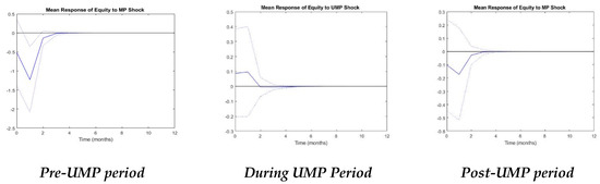
Figure 7.
Mean responses of equity prices in Asian developing economies to monetary policy shocks in pre-UMP, during UMP, and post-UMP periods.
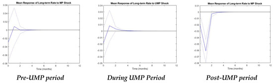
Figure 8.
Mean responses of long-term interest rates in Asian developing economies to monetary policy shocks in pre-UMP, during UMP, and post-UMP periods.
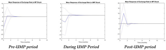
Figure 9.
Mean responses of exchange rates in Asian developing economies to monetary policy shocks in pre-UMP, during UMP, and post-UMP periods.
As can be seen from Figure 7, the response of equity prices in Asia to external shock is significantly positive once UMP is implemented. The other periods witness adverse reactions of equity prices to MP shock. This again confirms the existence of unconventional monetary effects from the US to Asian developing countries from 2008M9 to 2014M1.
In line with theory expectations, long-term interest rates in Asian developing countries respond negatively to the UMP shocks from the US, on impact. While Bowman et al. (2015) indicate that sovereign yields in emerging countries are significantly influenced by UMP shocks, our study does not find a substantial impact of the UMP shocks on long-term rates in Asian developing countries. MacDonald (2017) emphasizes that the market frictions can be balanced by the capital controls, leaving results somewhat diversified. The differences might stem from different methods, different samples, and the date of analysis.
During the UMP period, local interest rates immediately decline by around 0.02% before returning to the baseline in less than nine months. The influence of monetary policy shocks is trivial during the UMP period, in comparison with other phases. In addition, there has not been a significant difference in the mean responses of interest rates between pre-UMP and during UMP periods. As the long-term interest rate is not a fast-moving variable, this result seems to be reasonable. The spillover effect of UMP shocks on long-term interest rates in Asian developing countries seems to be ambiguous.
Concerning the changes of local currencies versus the USD dollar, these empirical results indicate that the UMP in the US appreciates the value of currencies in Asian developing countries. This study is consistent with previous papers (Glick and Leduc 2012; Punzi and Chantapacdepong 2019) that suggest external monetary shocks put an upward pressure on currency values in the recipient countries. Strikingly, similar to the mean responses of equity prices, there has been significant differences in the responses of exchange rates in these countries to monetary shocks between unconventional and conventional periods. Specifically, as can be seen from Figure 9, while UMP shocks from the US result in an appreciation of local currencies, MP shocks seem to exert adverse effects. Such an appreciation of domestic currencies might reduce the competitiveness of Asian developing countries in terms of export volume. Punzi and Chantapacdepong (2019) also suggest that this situation can be the source of financial vulnerability in the recipient countries. However, in comparison to the pre-UMP and during UMP periods, the size of responses in 2008M9–2014M1 is fairly small, which might not lead to severe consequences.
All in all, the spillover effects of the US UMP shocks do exist on the Asian developing markets, even though the magnitude of shocks is relatively small, which accords with Rafiq (2015). This result somehow supports the finding of Chudik and Fratzscher (2011) that the liquidity shocks from the US tend to influence other developed countries rather more strongly than developing markets.
6. Robustness Check8
For a robustness check, we alternate the SSR measured by Krippner (2013) by the SSR formulated by Wu and Xia (2016). The SSR by Wu and Xia (2016) follows a factor structure, which could capture rich information from a large dataset. The monetary policy shocks estimated by the SSR of Wu and Xia (2016) also significantly affect asset prices in Asian developing countries. During the UMP period, the SSR shock from the US leads to an increase in stock prices and appreciation of local currencies in Asian developing countries on impact. In addition, long-term bond yields witness a slight drop during 2008M9–2014M1 in these recipient countries, which is under the spillover effect of UMP surprises. Additionally, we implement another robustness check by excluding China. The empirical findings remain almost unchanged.
In sum, the results are robust to different measures of SSR and found that, on average, the UMP shocks also impose a small effect on long-term interest rates in these Asian developing nations, during 2008M9–2014M1, which is similar to the main analysis shown previously.
7. Conclusions
Our paper mainly examines the spillover effect of UMP shock from the US on Asian developing countries with consideration of different asset prices. The empirical findings suit well with what is expected from theories.
The first contribution of this research is to study the impact of UMP shock on three different asset prices, which meaningfully contributes to the literature. In line with theoretical predictions, during the period of UMP, a monetary shock is linked with an increase in equity prices, a decline in interest rates, and an appreciation of local currencies in Asian developing markets. These results confirm the existence of a spillover effect from US to its partner countries through transmission mechanisms including the exchange rate channel, portfolio rebalancing channel, and liquidity channel. The influence of UMP shocks seems to entirely disappear in Asian developing countries after 10 months. Additionally, the unconventional monetary policy from the US also helps boost economic growth and contemporaneously stabilize price levels in Asian developing countries.
Second, we found different spillover effects of the US monetary policy on Asian developing markets between unconventional and conventional periods. This result implies that policymakers in Asian developing countries should carefully consider the increasing capital inflows as it is a double-edged sword, challenging small open economies with a higher probability of severe problems such as an asset price bubble or current account deficit (Lee and Kim 2018). How to balance the excessive capital inflows and sustain economic growth is a complex question for developing countries to answer. Additionally, Asian developing countries might face a major risk caused by advanced economies winding down QE. Hence, policymakers in Asian developing economies should focus on strengthening macro-prudential policies for cross-border transactions, in order to mitigate the risk of volatile economic and financial conditions.
Up to this point, our research comes with some limitations regarding economic issues; such limitations suggest ideas for future studies. First, we did not address the effect of ‘sudden stop’ during the implementation of UMP. The risk of contagion triggered from advanced economies can threaten the economic growth in developing countries, especially those with high debt such as Malaysia and Thailand. Deeper research into the issue of contagion effects should be considered in future research. Second, this paper can be further developed by examining the spill back of capital from Asian developing nations to the US. Such large adverse cross-border effects can affect the US economy and the success of QE programs. Third, future studies might take into account whether the UMP shocks from other regions such as the UK, the Euro area, or Japan might interfere with the existing findings. These additional UMP shocks could be included in the existing model as control variables or employed in a separate model to compare with the US UMP shocks in terms of sign and magnitude.
Author Contributions
Investigation, methodology, writing—review/editing and supervision, T.B.N.T.; data curation, investigation, methodology and writing—original draft, H.C.H.P. All authors have read and agreed to the published version of the manuscript.
Funding
This research received no external funding.
Conflicts of Interest
The authors declare no conflict of interest.
Appendix A
Table A1.
Data description and sources.
Table A1.
Data description and sources.
| Variable | Description | Source |
|---|---|---|
| For the US | ||
| SSR | Shadow short rates—measure of monetary policy stances | Krippner (2016), monthly frequency, end of period data. |
| Real GDP (billions of chained 2012 dollars) | Fred, Bloomberg, IMF | |
| VIX Index | Measure of volatility of stock market | Bloomberg |
| Long-term interest rate (%) | Fred, Bloomberg | |
| CPI | Consumer Price Index | Fred |
| For Asian Developing Countries | ||
| Stock price index | Measure of equity price | Bloomberg, last price |
| Real exchange rate | Expressed as the bilateral exchange rate vis-à-vis the US dollars, in real term | Bloomberg, last price |
| Long-term yield (%) | Long-term interest rate | Bloomberg, national sources |
| Trade linkage (%) | Exports plus imports divided by GDP of each country | Bloomberg, IMF |
| Financial linkage (%) | Expressed as the ratio of Foreign Direct Investment (FDI) from US to one country over GDP of each country | US Bureau of Economic Analysis |
| Real GDP (billion USD) | Control variable for macroeconomic conditions | Fred, Bloomberg, IMF |
| CPI | Consumer Price Index | Bloomberg, national sources |
Table A2.
Lag structure selection.
Table A2.
Lag structure selection.
| Criterion | Pre-UMP Period (2004M2–2007M12) | During UMP Period (2008M9–2014M1) | Post-UMP Period (2014M2–2018M4) | |||||
|---|---|---|---|---|---|---|---|---|
| Number of Lags | p = q = 1 | p = q = 2 | p = q = 1 | p = q = 2 | p = q = 1 | p = q = 2 | ||
| Panel VARX Model for: | ||||||||
| Equity prices | MBIC | −167.239 | −134.780 | −168.676 | −136.189 | −160.744 | −141.796 | |
| MAIC | −33.426 | −34.420 | −16.662 | −22.179 | −17.778 | −34.572 | ||
| MQIC | −86.954 | −74.566 | −76.292 | −66.901 | −74.439 | −77.068 | ||
| Long-term interest rates | MBIC | −136.2503 | −123.111 | −185.399 | −143.828 | −158.724 | −136.010 | |
| MAIC | −8.906 | −27.603 | −33.386 | −29.818 | −14.758 | −28.787 | ||
| MQIC | −60.135 | −66.025 | −93.016 | −74.54 | −71.419 | −71.283 | ||
| Exchange rates | MBIC | −138.819 | −86.269 | −186.939 | −146.062 | −183.003 | −153.842 | |
| MAIC | −5.006 | 14.090 | −34.926 | −32.052 | −40.037 | −46.618 | ||
| MQIC | −58.534 | −26.056 | −94.556 | −76.774 | −96.699 | −89.114 | ||
Table A3.
Unit root tests for panel data.
Table A3.
Unit root tests for panel data.
| Variables |
Pre-UMP Period (2004M2–2007M12) |
During UMP Period (2008M9–2014M1) |
Post-UMP Period (2014M2–2018M4) | |||
|---|---|---|---|---|---|---|
| Breitung Statistic (Lamda) | p-Value | Breitung Statistic (Lamda) | p-Value | Breitung Statistic (Lamda) | p-Value | |
| MP shocks | −3.407 | 0.003 | −5.887 | 0.000 | −3.678 | 0.000 |
| Equity9 | −7.438 | 0.000 | −2.494 | 0.063 | −9.123 | 0.000 |
| Long-term rate | −8.262 10 | 0.000 | −1.524 | 0.063 | −9.034 | 0.000 |
| Exchange rate | −5.161 | 0.000 | −1.532 | 0.063 | −4.829 | 0.000 |
| Growth | −5.640 | 0.000 | −9.582 | 0.000 | −6.136 | 0.000 |
| Inflation | −8.393 | 0.000 | −6.167 | 0.000 | −7.214 | 0.000 |
References
- Aizenman, Joshua, Mahir Binici, and Michael M. Hutchison. 2016. The transmission of Federal Reserve tapering news to emerging financial markets. International Journal of Central Banking 12: 317–56. [Google Scholar]
- Alpanda, Sami, and Serdar Kabaca. 2020. International spillovers of large-scale asset purchases. Journal of the European Economic Association 18: 342–91. [Google Scholar] [CrossRef]
- Amisano, Gianni, and Carlo Giannini. 1997. From VAR models to Structural VAR models. In Topics in Structural VAR Econometrics. Berlin/Heidelberg: Springer. [Google Scholar]
- Anaya, Pablo, Michael Hachula, and Christian J. Offermanns. 2017. Spillovers of U.S. Unconventional Monetary Policy to Emerging Markets: The Role of Capital Flows. Journal of International Money and Finance 73: 275–95. [Google Scholar] [CrossRef]
- Andrews, Donald W. K., and Biao Lu. 2001. Consistent model and moment selection procedures for GMM estimation with application to dynamic panel data models. Journal of Econometrics 101: 123–64. [Google Scholar] [CrossRef]
- Bacchiocchi, Emanuele, Efrem Castelnuovo, and Luca Fanelli. 2017. Gimme a Break! Identification and Estimation of the Macroeconomic Effects of Monetary Policy Shocks in the U.S. Macroeconomic Dynamics. [Google Scholar] [CrossRef]
- Bauer, Michael D., and Christopher J. Neely. 2014. International Channels of the Fed’s Unconventional Monetary Policy. Journal of International Money and Finance 44: 24–46. [Google Scholar] [CrossRef]
- Bauer, Michael D., and Glenn D. Rudebusch. 2014. The Signaling Channel for Federal Reserve Bond Purchases. International Journal of Central Banking 10: 233–89. [Google Scholar] [CrossRef]
- Belke, Ansgar, Walter Orth, and Ralph Setzer. 2010. Liquidity and the dynamic pattern of asset price adjustment: A global view. Journal of Banking and Finance 34: 1933–45. [Google Scholar] [CrossRef]
- Bernanke, Ben S., and Blinder Alan S. 1992. The federal funds rate and the channels of monetary transmission. American Economic Review 82: 901–21. [Google Scholar]
- Bhattarai, Saroj, Arpita Chatterjee, and Woong Yong Park. 2018. Effects of US Quantitative Easing on Emerging Market Economies. Tokyo: Working Paper ADB Institute. [Google Scholar]
- Bhuiyan, Rokon. 2012. The Effects of Monetary Policy Shocks in Bangladesh: A Bayesian Structural VAR Approach. International Economic Journal 26: 301–16. [Google Scholar] [CrossRef]
- Black, Fischer. 1995. Interest Rates as Options. Journal of Finance 50: 1371–76. [Google Scholar] [CrossRef]
- Bowman, David, Juan M. Londono, and Horacio Sapriza. 2015. U.S. Unconventional Monetary Policy and Transmission to Emerging Market Economies. Journal of International Money and Finance 55: 27–59. [Google Scholar] [CrossRef]
- Brana, Sophie, Marie-Louise Djigbenou, and Stéphanie Prat. 2012. Global excess liquidity and asset prices in emerging countries: A PVAR approach. Emerging Markets Review 13: 256–67. [Google Scholar] [CrossRef]
- Breitung, Jörg. 2000. The local power of some unit root tests for panel data. In Advances in Econometrics, Volume 15: Nonstationary Panels, Panel Cointegration, and Dynamic Panels. Edited by Badi Hadi Baltagi. Amsterdam: JAI Press, pp. 161–78. [Google Scholar]
- Breitung, Jorg, Ralf Brüggemann, and Helmut Lütkepohl. 2004. Structural vector autoregressive modelling and impulse responses. In Applied Time Series Econometrics. Edited by H. Lütkepohl and M. Krãtzig. Cambridge: Cambridge University Press, pp. 159–96. [Google Scholar]
- Cavallari, Lilia, and Stefano D’Addona. 2015. Trade margins and exchange rate regimes: New evidence from a Panel VARX model. In Achieving Dynamism in an Anaemic Europe. Cham: Springer, pp. 29–48. [Google Scholar] [CrossRef]
- Cho, Dongchul, and Changyong Rhee. 2014. Effects of Quantitative Easing on Asia: Capital Flows and Financial Markets. Singapore Economic Review 59: 1–23. [Google Scholar] [CrossRef]
- Christensen, Jens H. E., and Glenn D. Rudebusch. 2012. The Response of Interest Rates to US and UK Quantitative Easing. Economic Journal 122: 385–414. [Google Scholar] [CrossRef]
- Christiano, Lawrence J., Martin Eichenbaum, and Charles Evans. 1996. The effects of monetary policy shocks: Evidence from the flow of funds. Review of Economics and Statistics 78: 16–34. [Google Scholar] [CrossRef]
- Chudik, Alexander, and Marcel Fratzscher. 2011. Identifying the global transmission of the 2007-09 financial crisis in a GVAR model. European Economic Review 55: 325–39. [Google Scholar] [CrossRef]
- Dahlhaus, Tatjana, Kristina Hess, and Abeer Reza. 2018. International Transmission Channels of U.S. Quantitative Easing: Evidence from Canada. Journal of Money, Credit and Banking 50: 545–63. [Google Scholar] [CrossRef]
- Damjanović, Milan, and Igor Masten. 2016. Shadow Short Rate and Monetary Policy in the Euro Area. Empirica 43: 279–98. [Google Scholar] [CrossRef]
- Doh, Taeyoung. 2010. The Efficacy of Large-Scale Asset Purchases at the Zero Lower Bound. Economic Review 95: 5–34. Available online: http://core.kmi.open.ac.uk/download/pdf/6380770.pdf (accessed on 16 March 2020).
- Doh, Taeyoung, and Jason Choi. 2016. Measuring the stance of monetary policy on and off the zero lower bound. Economic Review (Kansas City) 101: 5. [Google Scholar]
- Dornbusch, Rudiger. 1976. Expectations and exchange rate dynamics. Journal of Political Economy 84: 1161–76. [Google Scholar] [CrossRef]
- Eickmeier, Sandra, and Boris Hofmann. 2013. Monetary policy, housing booms, and financial (im) balances. Macroeconomic Dynamics 17: 830–60. [Google Scholar] [CrossRef]
- Fleming, J. Marcus. 1962. Domestic Financial Policies Under Fixed and Under Floating Exchange Rates Politiques. Staff Papers-International Monetary Fund 9: 369–80. [Google Scholar] [CrossRef]
- Fomby, Thomas, Yuki Ikeda, and Norman Loayza. 2013. The growth aftermath of natural disasters. Journal of Applied Econometric 28: 412–34. [Google Scholar] [CrossRef]
- Fratzscher, Marcel. 2012. Capital flows, push versus pull factors and the global financial crisis. Journal of International Economics 88: 341–56. [Google Scholar] [CrossRef]
- Fratzscher, Marcel, Marco Lo Duca, and Roland Straub. 2018. On the International Spillovers of US Quantitative Easing. Economic Journal 128: 330–77. [Google Scholar] [CrossRef]
- Frenkel, Jacob A., and Assaf Razin. 1987. The Mundell-Fleming model a quarter century later: A unified exposition. Staff Papers 34: 567–620. [Google Scholar] [CrossRef]
- Friedman, Milton, and Anna Jacobson Schwartz. 2008. A monetary History of the United States. Princeton: Princeton University Press. [Google Scholar]
- Gagnon, Joseph, Matthew Raskin, Julie Remache, and Brian Sack. 2011. The Financial Market Effects of the Federal Reserve’s Large-Scale Asset Purchases. International Journal of Central Banking 7: 3–43. [Google Scholar]
- Gambacorta, Leonardo, Boris Hofmann, and Gert Peersman. 2014. The Effectiveness of Unconventional Monetary Policy at the Zero Lower Bound: A Cross-Country Analysis. Journal of Money, Credit and Banking 46: 615–42. [Google Scholar] [CrossRef]
- Glick, Reuven, and Sylvain Leduc. 2012. Central Bank Announcements of Asset Purchases and the Impact on Global Financial and Commodity Markets. Journal of International Money and Finance 31: 2078–101. [Google Scholar] [CrossRef]
- Hamilton, James D., and Jing C. Wu. 2012. The Effectiveness of Alternative Monetary Policy Tools in a Zero Lower Bound Environment. Journal of Money, Credit and Banking 44: 3–46. [Google Scholar] [CrossRef]
- Hancock, Diana, and Wayne Passmore. 2011. Did the Federal Reserve’s MBS Purchase Program Lower Mortgage Rates? Journal of Monetary Economics 58: 498–514. [Google Scholar] [CrossRef]
- Hausman, Joshua, and Jon Wongswan. 2011. Global Asset Prices and FOMC Announcements. Journal of International Money and Finance 30: 547–71. [Google Scholar] [CrossRef]
- Herzer, Dierk, and Sebastian Vollmer. 2012. Inequality and growth: Evidence from panel cointegration. The Journal of Economic Inequality 10: 489–503. [Google Scholar] [CrossRef]
- Holtz-Eakin, Douglas, Whitney Newey, and Harvey S. Rosen. 1988. Estimating vector autoregressions with panel data. Econometrica 56: 1371–95. [Google Scholar] [CrossRef]
- Im, Kyung So, M. Hashem Pesaran, and Yongcheol Shin. 2003. Testing for unit roots in heterogeneous panels. Journal of Econometrics 115: 53–74. [Google Scholar] [CrossRef]
- Inoue, Atsushi, and Barbara Rossi. 2019. The Effects of Conventional and Unconventional Monetary Policy on Exchange Rates. Journal of International Economics 118: 419–47. Available online: https://econpapers.repec.org/RePEc:eee:inecon:v:118:y:2019:i:c:p:419-447 (accessed on 16 March 2020). [CrossRef]
- Joyce, Michael, Ana Lasaosa, Ibrahim Stevens, and Matthew Tong. 2011. The Financial Market Impact of Quantitative Easing in the United Kingdom. International Journal of Central Banking 7: 113–61. [Google Scholar]
- Kawai, Masahiro. 2015. International Spillovers of Monetary Policy: US Federal Reserve’s Quantitative Easing and Bank of Japan’s Quantitative and Qualitative Easing. SSRN Electronic Journal. [Google Scholar] [CrossRef]
- Khatiwada, Sameer. 2017. Quantitative Easing by the Fed and International Capital Flows. IHEID Working Paper, No. 02-2017. Available online: http://repec.graduateinstitute.ch/pdfs/Working_papers/HEIDWP02-2017.pdf (accessed on 16 March 2020).
- Kim, Soyoung. 2001. International Transmission of U.S. Monetary Policy Shocks: Evidence from VAR’s. Journal of Monetary Economics 48: 339–72. [Google Scholar] [CrossRef]
- Kim, Soyoung, and Nouriel Roubini. 2000. Exchange rate anomalies in the industrial countries: A solution with a structural VAR approach. Journal of Monetary Economics 45: 561–86. [Google Scholar] [CrossRef]
- Krippner, Leo. 2013. Measuring the Stance of Monetary Policy in Zero Lower Bound Environments. Economics Letters 118: 135–38. [Google Scholar] [CrossRef]
- Krippner, Leo. 2016. Documentation for Measures of Monetary Policy; Wellington: Reserve Bank of New Zealand. Available online: https://www.rbnz.govt.nz/-/media/ReserveBank/Files/Publications/Research/additional-research/leo-krippner/5892888.pdf (accessed on 16 March 2020).
- Krishnamurthy, Arvind, and Annette Vissing-Jorgensen. 2011. The Effects of Quantitative Easing on Interest Rates: Channels and Implications for Policy. Brookings Papers on Economic Activity 287: 215–87. [Google Scholar] [CrossRef]
- Lee, Il Houng, and Kyunghun Kim. 2018. Exchange Rate Flexibility, Financial Market Openness, and Economic Growth. Asian Economic Papers 17: 145–62. [Google Scholar] [CrossRef]
- Leeper, Eric M., Christopher A. Sims, Tao Zha, Robert E. Hall, and Ben S. Bernanke. 1996. What does monetary policy do? Brookings Papers on Economic Activity 1996: 1–78. [Google Scholar] [CrossRef]
- Lemke, Wolfgang, and Andreea Vladu. 2017. Below the Zero Lower Bound: A Shadow-Rate Term Structure Model for the Euro Area. In ECB Working Paper No. 1991. Frankfurt: European Central Bank. [Google Scholar]
- Lombardi, Marco J., and Feng Zhu. 2018. A shadow policy rate to calibrate US monetary policy at the zero lower bound. International Journal of Central Banking 14: 305–46. [Google Scholar]
- Lorenzoni, Guido. 2008. Inefficient Credit Booms. Review of Economic Studies 75: 809–33. [Google Scholar] [CrossRef]
- MacDonald, Margaux. 2017. International Capital Market Frictions and Spillovers from Quantitative Easing. Journal of International Money and Finance 70: 135–56. [Google Scholar] [CrossRef]
- Macdonald, Margaux, and Michał Ksawery Popiel. 2017. Unconventional Monetary Policy in a Small Open Economy. In IMF Working Paper 17/268. Washington, DC: International Monetary Fund. [Google Scholar]
- Maddala, Gangadharrao S., and Shaowen Wu. 2001. A comparative study of unit root tests with panel data and a new simple test. Oxford Bulletin of Economics and Statistics 61: 631–52. [Google Scholar] [CrossRef]
- Matousek, Roman, Stephanos T. Papadamou, Aleksandar Šević, and Nickolaos G. Tzeremes. 2019. The effectiveness of quantitative easing: Evidence from Japan. Journal of International Money and Finance 99: 102068. [Google Scholar] [CrossRef]
- Miyajima, Ken, Madhusudan S. Mohanty, and James Yetman. 2014. Spillovers of US Unconventional Monetary Policy to Asia: The Role of Long-Term Interest Rates. In BIS Working Paper No. 478. Available online: https://ssrn.com/abstract=2542229 (accessed on 16 March 2020).
- Morgan, Peter. 2011. Impact of US Quantitative Easing Policy on Emerging Asia. In ADBI Working Paper 321. Tokyo: Asian Development Bank Institute. [Google Scholar]
- Mundell, Robert A. 1963. Capital Mobility and Stabilization Policy under Fixed and Flexible Exchange Rates. The Canadian Journal of Economics and Political Science/Revue Canadienne d’Economique et de Science Politique 29: 475–85. [Google Scholar] [CrossRef]
- Neely, Christopher J. 2015. Unconventional Monetary Policy Had Large International Effects. Journal of Banking and Finance 52: 101–11. [Google Scholar] [CrossRef]
- Nickell, Stephen. 1981. Biases in dynamic models with fixed effects. Econometrica: Journal of the Econometric Society 49: 1417–26. [Google Scholar] [CrossRef]
- Park, Donghyun, Arief Ramayandi, and Kwanho Shin. 2013. Why Asia Fare Better during the Global Financial Crisis than during the Asian Financial Crisis? Peterson Institute for International Economics 2013: 103–39. Available online: www.piie.com (accessed on 16 March 2020).
- Pedroni, Peter. 2013. Structural Panel VARs. Econometrics 1: 180–206. [Google Scholar] [CrossRef]
- Pham, Trinh T. T., and Phuc T. Nguyen. 2019. Monetary Policy Responses of Asian Countries to Spillovers from US Monetary Policy. Asian-Pacific Economic Literature 33: 78–97. [Google Scholar] [CrossRef]
- Punzi, Maria Teresa, and Pornpinun Chantapacdepong. 2019. Spillover Effects of Unconventional Monetary Policy on Asia and the Pacific. In Macroeconomic Shocks and Unconventional Monetary Policy: Impacts on Emerging Markets. Oxford: Oxford University Press, pp. 182–215. [Google Scholar]
- Rafiq, Sohrab. 2015. The Effects of U.S. Unconventional Monetary Policy on Asia Frontier Developing Economies. IMF Working Papers 15: 1. [Google Scholar] [CrossRef]
- Romer, Christina D., and David H. Romer. 2004. A new measure of monetary shocks: Derivation and implications. American Economic Review 94: 1055–84. [Google Scholar] [CrossRef]
- Rudebusch, Glenn D. 1998. Do measures of monetary policy in a VAR make sense? International Economic Review 39: 907–31. [Google Scholar] [CrossRef]
- Sims, Christopher. A. 1980. Macroeconomics and Reality. Econometrica 48: 1–48. [Google Scholar] [CrossRef]
- Sims, Christopher A., and Tao Zha. 2006. Were There Regime Switches in U.S. Monetary Policy? The American Economic Review 96: 54–81. Available online: http://www.jstor.org/stable/30034354 (accessed on 16 March 2020). [CrossRef]
- Stock, James H., and Mark W. Watson. 2001. Vector Autoregressions. Journal of Economic Perspectives 15: 101–15. [Google Scholar] [CrossRef]
- Tillmann, Peter. 2015. Unconventional monetary policy and the spillovers to emerging markets. Journal of International Money and Finance 66: 136–56. [Google Scholar] [CrossRef]
- Wolfers, Justin. 2014. The Fed has not stopped trying to stimulate the economy. The New York Times. Available online: https://www.nytimes.com/2014/10/30/upshot/the-fed-has-not-stopped-trying-to-stimulate-the-economy.html (accessed on 16 March 2020).
- Wright, Jonathan H. 2012. What Does Monetary Policy Do to Long-Term Interest Rates at the Zero Lower Bound? Economic Journal 122: 447–66. [Google Scholar] [CrossRef]
- Wu, Jing Cynthia, and Fan Dora Xia. 2016. Measuring the Macroeconomic Impact of Monetary Policy at the Zero Lower Bound. Journal of Money, Credit and Banking 48: 253–91. [Google Scholar] [CrossRef]
- Xu, Ying, and Hai Anh La. 2019. Spillovers of the United States’ Unconventional Monetary Policy to Emerging Asia. In Macroeconomic Shocks and Unconventional Monetary Policy: Impacts on Emerging Markets. Oxford: Oxford University Press, pp. 118–45. [Google Scholar]
| 1 | In this study, we will use QE and LSAPs interchangeably. |
| 2 | Agency securities refer to bonds and notes issued by the government or the national mortgage associations such as Fannie Mae and Freddie Mac. Moreover, these securities are considered as the second quality debts instruments. |
| 3 | The IS–LM model refers to the interaction among countries by exploring the international transmission. An expansion in government purchases causes the IS curve to shift to the right, resulting in an upward turn in the interest rate in the home country. |
| 4 | QE1, QE2, and QE3 are used to refer to quantitative easing programs that occurred in the first, second, and third phases of implementation, respectively. |
| 5 | We exclude Pakistan, Taiwan, Bangladesh, and Sri Lanka due the lack of data. |
| 6 | Especially for this variable, we later take its logarithm instead to stabilize the variance of the underlying series. |
| 7 | A panel-data unit-root test. |
| 8 | Results available upon request. |
| 9 | For the purpose of compactness, we just present the unit root tests for asset prices which have been taken the first differences already. |
| 10 | We employ the IPS unit root test instead, the statistic refers to ‘z-t-tilde-bar’. |


© 2020 by the authors. Licensee MDPI, Basel, Switzerland. This article is an open access article distributed under the terms and conditions of the Creative Commons Attribution (CC BY) license (http://creativecommons.org/licenses/by/4.0/).