Article

Is Investors’ Psychology Affected Due to a Potential Unexpected Environmental Disaster?

Laboratory of Operations Research, Department of Economics, University of Thessaly, 38333 Volos, Greece
*
Author to whom correspondence should be addressed.
J. Risk Financial Manag. 2020, 13(7), 151; https://doi.org/10.3390/jrfm13070151
Submission received: 9 June 2020 / Revised: 7 July 2020 / Accepted: 10 July 2020 / Published: 12 July 2020
(This article belongs to the Special Issue Risk and Financial Consequences)

Abstract

:
The purpose of this paper is to approach the way investors perceive the risk associated with unexpected environmental disasters. For that reason, we examine certain types of natural and technological disasters, also known as “na-tech”. Based on the existing relevant literature and historical sources, the most common types of such disasters are geophysical and industrial environmental disasters. After providing evidence of the historical evolution of the na-tech events and a brief description of the events included in the sample, we estimate the systematic risk of assets connected to these events. The goal is to capture possible abnormalities as well as to observe investors’ psychology of risk after the occurrence of an unexpected event. Finally, we examine whether macroeconomic factors may affect those abnormalities. The empirical findings indicate that the cases we examined did not cause significant cumulative abnormal returns. Moreover, some events caused an increase in systematic risk while surprisingly some others reduced risk, showing that investors tend to support a country and/or corporation due to their reputation.

1. Introduction

Among those studying or working in the financial sector there is a well-spread knowledge regarding the rational investors’ preferences. Regardless of the business sector they invest in, investors’ main goal is to maximize their profits, being characterized as “risk averters” (Merton 1969; Benartzi and Thaler 1999; Campbell and Cochrane 1999; Aıt-Sahalia and Lo 2000; Jackwerth 2000; Rosenberg and Engle 2002; Brandt and Wang 2003; Gordon and St-Amour 2004; Bliss and Panigirtzoglou 2004; Bollerslev et al. 2011; Halkos et al. 2017). Investors are usually assumed to be rational, so if we ignore the arbitrage case, they tend to choose more “safe” investments which will allow them to maximize their profits, or in other words minimize potential risk they receive by investing (Cohn et al. 1975; Benartzi and Thaler 1995; Haigh and List 2005).
Hedging and portfolio diversification may appear to be efficient in reducing the potential loss of an investment. Great attention has been drawn about the advantages of portfolio diversification (Bugár and Maurer 2002). Graham and Jennings (1987) mentioned the ability of transferring the risk of investment through hedging, while Bond and Thompson (1985) highlighted that the size of the optimal hedging ratio is one of the main determinants used by decision makers apart from cash position of the corporation.
Based on available information, such as credit rating, stability of the corporation or government, whether we are working with stocks or bonds, as well as investors’ preferences, diversification of portfolios and assurance of investors’ capital may be achieved. The first researcher who extended the Markovitz theoretical idea of the modern portfolio selection was Grubel (1968). We can use options or future derivatives concerning our predictions regarding, for instance, the value of exchange rates. However, there are some cases which cannot be predicted. The act of nature is such a case (Halkos and Zisiadou 2018).
Nature acts independently, and a common example of that independence is the tectonic plate movement (Halkos and Zisiadou 2018). Distinguished sciences, such as Geology and Seismology, have the techniques to monitor, observe, and examine the geophysical events caused by those tectonic plate movements. However, even those specialized sciences cannot predict the occurrence, and more specifically the exact place, epicenter, and intensity of an upcoming event. Thus, those actions which cannot be predicted may cause significant losses, both economic and life-related. Regarding economic losses, they can be due to many factors such as partial or total destruction of homes or business premises that will lead to reduced, if not zero, productivity.
Concerning the country that may be affected by such a situation, reduced productivity can cause a drastic decline in gross domestic product (GDP)1, as well as affect a country’s borrowing capacity and reliability, which tend to be depicted in its credit rating. As we have already mentioned, the credit rating of a country or corporation is one of the most common rates that mirror the potential risk the investor is about to perceive by investing in this specific bond or stock. In the case of businesses, reduced productivity may affect investors’ perceptions causing fluctuations in the share price or even volatility in its board of directors. Although disasters are associated with risk, investors tend to have a different perspective regarding the source of the disaster2.
More specifically, if a country is facing a natural disaster, where no one can be blamed, foreign investors who may hold this country’s bonds will continue to trust the country due to the “innocence” of the country. On the other hand, when a firm causes a technological disaster, such as a nuclear power plant explosion, investors will “punish” the firm by selling its shares at any price to avoid a bigger loss, if this corporation is publicly traded. In such cases, corporations may lose trustworthiness. Nevertheless, in some cases, the possible technological disaster is not a firm’s fault.
In the literature, these cases tend to be called “na-tech”, a term that actually depicts the source of the disaster. Sometimes, one natural disaster, caused by a tectonic plate movement, can lead to another natural or even technological disaster. For instance, a ground movement may lead to another earthquake3 at the seabed, known as a tsunami, or an earthquake, in general, may cause a dysfunction in a factory installation which may therefore cause an industrial disaster. A characteristic example is the case of Fukushima Daiichi Power Plant disaster, which will be analyzed in the following section.
The purpose of this paper is to approach the way investors perceive the risk associated with unexpected environmental disasters. More specifically, it examines certain types of natural and technological disasters which tend to be associated and are listed under the categories of geophysical and industrial disasters. The goal is to capture possible abnormalities as well as to observe investors’ psychology of risk after the occurrence of an unexpected event. Ultimately, we examine whether macroeconomic factors may affect those abnormalities. The structure of the paper is as follows. Section 2 reviews the existing relevant literature, while Section 3 provides the methodology and data used. In Section 4 the results of the analysis are presented and discussed. Finally, Section 5 concludes the study providing important statements and fundamentals for further research.

2. Literature Review

2.1. Geophysical and Industrial Hazards

Geophysical phenomena are not unexpected processes in terms of appearance and frequency. More specifically, since ancient times, the existence of these phenomena was known and commonly detected at a higher frequency in certain areas across the globe. The continuous movement of the Earth’s parts combined with weather condition changes have shaped the present image of the planet. Islands have been created or destroyed by volcanic eruptions, and landscapes have undergone changes from ground movements and tidal waves; however, the intensity of the event is the main factor affecting the final outcome.
Additionally, natural disasters cause a great number of fatalities as well as supreme national catastrophes (Viscusi 2009). An extended literature considering the terminology and high-risk areas was presented by Halkos and Zisiadou (2018). Based on the CRED (Centre for Research on the Epidemiology of Disaster) database, 1621 geophysical events have been recorded since 1900 causing 2,678,022 fatalities and economic damages, which aggregately exceeded 781.5 billion United States Dollar (USD) (EMDAT 2017; Halkos and Zisiadou 2018). The significance of a natural disaster to the economy was also emphasized by Lee et al. (2018), who described how possible natural disasters tend to cause volatility on stock markets.
Technological accidents, on the other hand, do not have similarities with the geophysical phenomena regarding expectancy. Nowadays, technology takes up more and more space in our lives, not only for professional but also for personal purposes. Of course, when it comes to technological accidents and disasters, the first thing that comes to mind is industrial accidents. What is important to mention is that, technological disasters include all types of accidents that may occur with technology as one of the main factors. The three main categories of technological accidents are industrial, miscellaneous, and transport accidents (Halkos and Zisiadou 2019).
Once again using the CRED database, we can come to the conclusion that industrial hazards are not the most frequent, however, they are the most disastrous. Over the last 117 years (1900–2016), 1434 industrial events have caused 57,619 fatalities and almost 43.1 billion USD economic damages (EMDAT 2017; Halkos and Zisiadou 2019). Industrial hazards, or even disasters, include all cases that may cause production disruption or even fatalities involving industrial buildings, such as chemical spills, collapses, explosions, fires, gas leaks, oil spills, poisoning, and radiation. What is really important to mention is that the number of fatalities became greater during the last years due to population increases in these high-risk areas (Kunreuther 1996).
Although there is a perception that natural phenomena are unexpected and occur randomly, there is evidence to suggest that, partially, the assertion of randomness is not valid. To be more specific, there is a proven regional distribution regarding geophysical events, initially mentioned by Bolt (1988) as the “Ring of Fire”. Based on the CRED database (EMDAT 2017) and with the use of R-studio packages and routines, maps of occurrence have been created both for geophysical and industrial hazards (Halkos and Zisiadou 2018, 2019). Figure 1a represents the space concentration of geophysical hazards in the high-risk area called the “Ring of Fire”.
In other words, although the exact place and time of an upcoming geophysical event cannot be predicted, based on evidence, we know a priori, which regions are more prone to face another disaster. Due to the possibility of a new catastrophe, governments should pay more attention to those high-risk areas as an attempt to reduce possible losses (Viscusi 2006). What is interesting though is that, although we were expecting a space concentration regarding natural events, the assertion of regional distribution is also observed in the case of industrial hazards. As seen in Figure 1b, East Asia is the most suffered region regarding industrial disasters. Although the reasons for such a space concentration are not known, based on evidence, researchers have at their disposal data that provide them with a first illustration of the riskiest areas.
As already mentioned, investors are primarily oriented to avoid most risk, or at least try to protect themselves from it. If they know, therefore, in advance, the risks they adopt by investing in those regions, they may be able to fully diversify their portfolios. Before analyzing the cases that will be used in our modeling, it is important to understand the basic concepts related to the seriousness of incidents included in our sample. The first basic requirement for sample creation is the date that each event occurred, as we included events from 2000 onwards for reasons of availability of stock data. The second, and equally important, reason is the intensity of each event.
Regarding the events we examine, there are four different intensity scales. For earthquakes, either ground movements or tsunamis, there are two different scales, the Moment Magnitude (Mw), also known as the Richter Scale, and the Intensity Scale, also known as the Mercalli Scale. These scales are most commonly used while measuring the intensity of a natural geophysical event. Regarding industrial events, to our knowledge, there is only one scale that is used as a tool to rate an industrial disaster. This scale is the International Nuclear and Radiological Event Scale (INES) which was created by the International Atomic Energy Agency (IAEA) and the Nuclear Energy Agency of the Organization for Economic Co-operation and Development (OECD/NEA) in 19904. The values of each scale and their impact are quite useful when describing an event and explaining the reason for inclusion in the sample.

2.2. Events of the Research

The survey sample contains 25 events, including 12 earthquakes, nine volcanic eruptions, and just four industrial disasters. The initial list of events that occurred since 2000 included more industrial accidents, however most cases were related to non-publicly listed corporations. These corporations have no available share price data which automatically excludes them from the sample of examination. Additionally, events before 2000 were also excluded due to the fact that open source databases barely have available historical data before that date. A significant number of industrial disasters has been excluded due to the fact that most of the corporations are not publicly listed, thus there are no stock prices available for market reactions estimation. Moreover, regarding geophysical disasters, the 2006 Indonesia earthquake was excluded from the research after observing anomalies in its behavior, and more specifically, negative systematic risk.
The first event of the analysis (Event 1) is the Denali earthquake in Alaska, USA on 3 November 2002 (Dunham and Archuleta 2004; Eberhart-Phillips et al. 2003; Jibson et al. 2006; Freed et al. 2006), with a Mw = 7.9 and a maximum intensity IX causing approximately 56 million USD in economic losses. This earthquake caused an estimated total damage of 20–56 million USD and one injury, while it triggered several landslides, with the worst of them causing a collision of 30 million m3 of rocks and ice (Eberhart-Phillips et al. 2003). The 2004 Indian Ocean earthquake, which took place in Thailand on 26 December 2004 (Event 2), with a Mw = 9.1–9.3 and a maximum intensity IX, caused an estimated total damage of 15 billion USD and 227,838 fatalities. The tsunami was created after the ground movement reached a 51 m wave. According to Telford and Cosgrave (2007), the most interesting evidence from the earthquake, that occurred over the Burma and Indian plate joint, was the immediate funding response across the globe. Wang and Liu (2006) characterized this geophysical event as one of the most devastating over the last 100 years. Moreover, they mentioned that the initial magnitude estimation was 9.0 which afterwards was updated to 9.1–9.3 while the waves created by the earthquake travelled at the speed of 700 Km/h.
In Pakistan, the Kashmir earthquake took place on 8 October 2005 (Event 3) with a Mw = 7.6 and a maximum intensity VII causing in economic damage as reported by the Asian Development Bank and the World Bank. The casualties of this disaster were 28 million displaced citizens, an estimation of 86,000–87,351 fatalities, and 6900–75,266 injuries citizens (Avouac et al. 2006). According to Kamp et al. (2008), the Kashmir earthquake triggered severe landslides, however, the majority of the fatalities were caused due to the inappropriate design of buildings and poor quality of construction materials. The aftermath of natural disasters regarding losses can be reduced by respecting and following the construction building codes (Priest 1996).
Based on Liu-Zeng et al. (2009), the 2008 Sichuan earthquake (12.05.2008) in China (Event 4) was a geophysical disaster with a Mw = 8.0 which devastated the western rim of Sichuan Basin. The maximum intensity of that earthquake was XI and the estimated total damage was 150 billion USD, with 87,587 fatalities, 374,643 injured, and 18,392 missing citizens. One of the most known and disastrous geophysical events of the new millennium was the tsunamigenic5 earthquake in Tohoku, Japan on 11 March 2011 (Event 5) which led to the greatest nuclear accident in recent years (after the case of Chernobyl) at the Fukushima Daiichi Nuclear Power Plant. The earthquake with Mw = 9.0–9.1 and maximum intensity IX created waves up to 40.5 m as well as landslides. The estimated total damage was 360 billion USD. The industrial case of the Daiichi disaster is described further in detail as Event 25. The estimated economic damage that occurred due to this disastrous event was approximately 360 billion USD, from which, 210 billion USD was recorded as due to the industrial disaster.
Moving forward, on 22 February 2011 in Christchurch in New Zealand, a Mw = 7.2 earthquake, which also led to a tsunami and landslides, caused 115 fatalities and 1500–2000 injuries. The maximum intensity of this event (Event 6) was IX. Bradley and Cubrinovski (2011) explained that New Zealand is located on the joint of the Pacific and Australian plates, two active tectonic plates with lateral sedimentations. This earthquake, together with the one that occurred on 23 December 2011 in New Zealand, caused an estimated 15–30 billion USD in damage.
Less than eight years after the devastating Indian Ocean earthquake in 2004, another Mw = 8.6 earthquake struck on 11 April 2012 in the Indian Ocean, however, this time the affected country was Indonesia (Event 7). Pollitz et al. (2012), mentioned that this earthquake, with a maximum intensity VII, 10 fatalities, and 12 injured citizens, was by far the largest strike-slip event, causing almost 9 billion USD in economic damage. The 2012 Indian Ocean earthquake was a tsunami associated event, as most of the cases examined in this paper, showing that natural events, or even disasters, are not individual incidents—nature interacts. The Illapel case was a Mw = 8.3 earthquake which affected both Chile and Argentina on 16 September 2015 with maximum intensity IX; it also created a tsunami. The aftermath of this earthquake in Chile was 15 fatalities and six missing citizens and 800 million USD in economic losses, while in Argentina there was only one fatality and few injured citizens (Event 8). Ruiz et al. (2016) mentioned that since the earthquake of Malue in 2010, there is an extensive post seismic distortion. Based on Heidarzadeh et al. (2016), the Illapel case raised a lot of attention and has been observed by the Pacific Tsunami Warning Center and the Japan Meteorological Agency. The tsunami, which was created by the earthquake in South America that affected Chile and Argentina, reached the coastlines of Japan, Hawaii, New Zealand, Vanuatu, and Australia.
Meanwhile, on 25 October 2010, Indonesia faced all three cases of geophysical disasters (Event 9). The Mentawai earthquake in Sumatra was a Mw = 7.8 earthquake, which led to a tsunami as well, that caused 408 fatalities and 303 missing citizens, but reported no economic losses. As Newman et al. (2011) mentioned, the Mentawai earthquake was characterized as a rare slow-source tsunami earthquake. On the same day, in the region near Java in Indonesia, one of the most active and hazardous volcanoes globally, Mount Merapi, erupted (Jousset et al. 2012). This volcanic eruption caused a chaotic situation regarding air traffic to the point that 2000 flights were cancelled. At the end of 2011, and more specifically, on 23 December 2011, New Zealand experienced another earthquake event (Event 10). As Bannister and Gledhill (2012) described, two ground movements took place in Christchurch 10 km and 15 km east from the city center, respectively, only 10 months after the first earthquake of the same year. The cumulative economic losses were 15–30 billion USD as previously mentioned.
On 21 July 2014, a lake tsunami occurred in Iceland and more specifically in Aksja, caused by volcanic activity (Event 11); no fatalities nor economic damage was recorded. Gylfadóttir et al. (2017) emphasized the unique phenomenon of a tsunami into a lake due to the rockslide that was released from the inner Askja caldera. The last earthquake included in the sample of analysis is the one that took place in Kaikoura, New Zealand on 14 November 2016 (Event 12). Once again, it was the joint of the Pacific and Australian plates, two active tectonic plates with lateral sedimentations, that created the Mw = 7.8 earthquake event with a maximum intensity IX which afterwards led to a tsunami causing two fatalities and 57 injured citizens (Hollingsworth et al. 2017). The economic impact of this event reached 613 million New Zealand Dollar (NZ$).
Moving forward, the next events included in the analysis are related to volcanic activity since 2000. On 7 August 2008, Kasatochi volcano (Event 13) in the USA erupted unexpectedly. Based on Waythomas et al. (2010), this specific volcano had no significant eruptions since then, however, the eruption of 2008 received a level 4 rating on the Volcanic Explosivity Index (VEI) scale. Almost a year later, another eruption received a level 4 rating. On 11 June 2009, in Russia, the Sarychev Peak erupted (Event 14). As Urai and Ishizuka (2011) mentioned, the Sarychev Peak is not monitored with ground-based instruments, however, the great eruption of 2009, which lasted almost eight days was captured by satellites. Iceland is very famous regarding volcanic activities. On 20 March 2010 and for 39 days (Event 15), a level 4 volcanic eruption took place in Eyjafjallajokull (Gudmundsson et al. 2012). Moreover, the next year, on 22 May 2011 (Event 16), another level 4 eruption occurred at the most active volcano in Iceland, Grimsvotn, located beneath the Vatnajokull ice sheet (Sigmarsson et al. 2013).
Scollo et al. (2014) and Viccaro et al. (2015) examined the Etna eruption on 05 March 2013 (Event 17) which received a level 3 rating on the VEI scale. In a period of two years, Etna in Italy produced 38 basaltic lava fountains. According to Viccaro et al. (2015), the volcanic activity started after eight months of rest. Kato et al. (2015) analyzed the Mount Ontake, Japan, volcanic eruption on 27 September 2014 (Event 18), that caused the deaths of 57 climbers. The number of fatalities increased since six more missing climbers were assumed to be dead. Kaneko et al. (2016) characterized this eruption as a small eruption with a short period; since it received a level 3 rating, it has not been examined thoroughly, thus the causes remain unknown. The volcanic eruption of Kelud, Indonesia on 13 February 2014 (Event 19), raised a lot of attention as it was characterized as the most powerful eruption of the decade (Caudron et al. 2015) causing 185 million USD in economic damage compared to all previous volcanic activities that had no reported economic impacts. A historic eruption was the one of Calbuco, Chile on 22 April 2015 (Event 20) since it did not have any recorded eruption in the last 43 years (Van Eaton et al. 2016). Due to the eruption, volcanic ash was dispersed in Chile, Argentina, and Uruguay. Ivy et al. (2017) observed a change in the ozone hole caused by that eruption, which also reported 600 million USD in economic losses. The last volcanic eruption included in the sample is that of Sinabung (Event 21) on 22 May 2016. Sinulingga and Siregar (2017) mentioned that Sinabung is one of 130 volcanoes in Indonesia; it lies on the Ring of Fire, which is a high-risk area concerning earthquakes.
The final category of the events included in the sample are related to industrial accidents. Only four events were included in the analysis due to the fact that the rest of the corporations, which caused industrial disasters, are not publicly listed. Three of those events are oil spills while the last event is the greatest nuclear disaster in recent years, and one of the two greatest disasters in history. Event 22 is the Prudhoe Bay oil spill caused by BP on 2 March 2006. Based on Kurtz (2010), this specific oil spill was the largest pipeline incident in the history of the operating system. The reputation of BP suffered from this incident and four years after the first oil spill of the new millennium, a new oil spill, this time in the Gulf of Mexico, occurred and aggravated the existing situation. Moreover, BP was forced to pay a 25 million USD fine for the environmental disaster. On 20 April 2010, Deepwater Horizon (Event 23), caused 11 fatalities and 17 injuries, as well as an environmental disaster due to the 2.1 million gallons of dispersants on the surface and wellhead of the Gulf of Mexico (Kujawinski et al. 2011). This time the economic impact for BP was dramatically increased compared to the previous event. The corporation had to pay 70 billion USD in fines and cleanup costs, while at the same time the market value of the corporation faced a sharp decrease. Three years later, on 29 March 2013, the Mayflower oil spill (Event 24) caused by Exxon Mobil, released more than 5000 barrels of crude oil. Based on Droitsch (2014), 1.36 million gallons of crude oil have proven very difficult to clean up. The fine that Exxon Mobil was forced to pay equaled 5 million USD.
Last, but not least, is the nuclear disaster of the Fukushima Daiichi Nuclear Power Plant that occurred on 11 March 2011, after the Tohoku earthquake and tsunami that reached the coast of Japan. Due to the earthquake 11 nuclear power plants stopped their operations. The cooling system of Fukushima’s power plant also stopped operating, causing the mot catastrophic nuclear accident after the one in Chernobyl. As already mentioned, 210 billion USD of the 360 billion USD recorded as economic damage were due to this industrial disaster and not due to the tsunami. Initially, the Fukushima Daiichi disaster received a level 5 rating on the International Nuclear and Radiological Event Scale (INES), but after the reassessment of the situation, Fukushima disaster received a level 7 rating. Till that day, only Chernobyl had a level 7 rating (Norio et al. 2011).

2.3. Proposed Methodologies

The process of modeling has never been easy. Of course, it may become even more lax and chaotic if qualitative variables are included in the study, which may not be measurable (such as the investor’s psychology, credibility of a government, and reputation of a business). Of course, with appropriate econometric methods and use of specific variables, we can partially integrate qualitative variables in our models. Although one factor that cannot be modeled is randomness. From a theoretical point of view, it is expected that we cannot model and therefore predict the “unexpected” because then it would cease to be a random event. Randomness, and consequently uncertainty, are what characterize markets. However, significant efforts have been made to evaluate models that can determine the expected value of an asset.
The most known models are the market model, arbitrage pricing theory (APT), and capital asset pricing model (CAPM)6. Regarding cases where unexpected events or announcements occur, event study analysis initially proposed by MacKinlay (1997) is the most common method estimating abnormality on returns (Prabhala 1997; Binder 1998; Maloney and Mulherin 2003; Gaspar et al. 2005; Karolyi and Martell 2010; Charles and Darné 2006; Walker et al. 2006; Arin et al. 2008; Brounen and Derwall 2010; Carpentier and Suret 2015; Halkos et al. 2017).
Of these three approaches, the preferred one is the CAPM. Most financial advisors as well as many researchers tend to use it in order to estimate systematic risk of each stock or bond (Strong 1992; Faff 1991; Fernald and Rogers 2002; Chen 2003; Womack and Zhang 2003; Fernandez 2006; Bruner et al. 2008; Adrian and Franzoni 2009). By estimating systematic risk, we can therefore predict expected returns of the asset examined, as well as abnormal returns using the actual value of return. When an unexpected event occurs, the question raised is whether those abnormal returns tend to be significant, showing the reaction, either positive or negative, of investors. This is the main path to follow in our analysis.

3. Methodology

3.1. Hypotheses and Data

Carter and Simkins (2004) decided to investigate airline stocks after the terrorist attacks on 11 September 2001. Their findings provide information regarding the USA capital market and the returns of airline corporations. They found that after the attack, statistically significant negative abnormal returns were observed for the examined airlines. Based on that outcome, we intend to observe if the under-investigation assets follow the same path (Hypothesis 1). Another significant finding by Carter and Simkins (2004) is that the results indicated a rapid drop of stock prices which led to a shock of the USA capital markets. Based on that finding, we seek to examine whether an unexpected disaster can have a similar impact on the government’s bond price or the share price of a corporation7 (Hypothesis 2).
Moving forward, the psychological impact of an unexpected event, which in Carter and Simkins’ (2004) case is the September 11th attack, may trigger the rationality that characterizes investors and leads them to react immediately causing pricing volatility. However, it is proven by evidence that larger airline corporations took advantage of that event, while smaller airline corporations did not have that opportunity. On the same path, we shall observe if such a condition is feasible at a country level (Hypothesis 3). Finally, Carter and Simkins (2004) investigated the impact of corporations’ size to market reaction giving us the priming to include countries’ economic status and its impact on the investors’ psychology (Hypothesis 4).
The first step of our analysis is to put the underlying assumptions to determine both the course of analysis and the time interval and variables to be used. The main hypotheses that will be examined here as follows:
Hypothesis 1 (H1).
There is no significant abnormal return after an unexpected na-tech disaster.
Hypothesis 2 (H2).
The systematic risk of an asset remains unaffected by an unexpected na-tech disaster.
Hypothesis 3 (H3).
Macroeconomic factors of the country suffering from an unexpected na-tech disaster cannot influence investors’ psychology and decisions.
Hypothesis 4 (H4).
The status of an economy does not affect investors’ decision.
For examining the above hypotheses, both financial and macroeconomic data are used. Regarding financial data, it is important to mention that daily stock and bond prices have been derived from open-source databases8 with a time-span of 125 days before the occurrence of the event as well as three days after the occurrence of the event to capture the possible return abnormality. When the event of analysis belongs to a natural disaster, the asset of examination is the country’s government bond, while the market index used is the corresponding Government Bond Index. In order to collect the bond data, we searched for data related to the government bond with longer time-to-maturity of each country facing a disaster. However, in some cases, the longer time-to-maturity bond had stable (same) bond price values, which would have given us bond returns equal to zero. In those cases, the exact previous bond was selected and included in our analysis. Restrictions regarding the open source data, possible exclusion of events due to lack of data, and the unavailability of dividend yields and/or stock splits have undoubtedly affected our final estimations. When the event of analysis belongs to a technological disaster, the asset of examination is the corporation’s stock price, while the market index used is the corresponding market index which the corporation is listed in.
Concerning the risk-free asset that is necessary for the CAPM approach, the assumption of Barro and Misra (2016) was used; they underlined that gold can be considered as a risk-free asset since it cannot be used as a hedge against macroeconomic declines and its expected real rate of return should be close to risk-free. As already mentioned, some events have been excluded from the analysis due to lack of information, mainly because corporations are not publicly listed, or due to overlapping cases, where the examination window of one event overlaps with the estimation window of another in the same country. Using this open-source database, confronts us with the main limitation of the research, in terms of time span. This is the main reason we chose na-tech disasters which occurred since 2000. For the macroeconomic factors’ variables, the reliable and recognized database of the World Bank9 was used.

3.2. Event Study Analysis

The most widespread method for analysis of the market reactions is the event study analysis as described by MacKinlay (1997). The initial step for the following analysis is to set the estimation and the event windows. As an event window, we used a seven-day period (−3, +3) centered to the event day10 and including three days before and three days after the event, in an attempt to capture market reaction to the disaster. This event window will be used to estimate the expected return of the asset as well as the possible abnormality. As an estimation window, we used a 120-day period (−124, −4), which should not include the days of the event window. By establishing a wider estimation window, compared to the time span proposed by MacKinlay (1997), we estimated the systematic risk before the occurrence of the event with higher accuracy. This approach allowed us to predict more precisely the expected returns of the assets on the seven-day event window and these expected returns provided more accurate abnormal returns. After calculating systematic risk, we moved forward to the event window to approach abnormal returns.
The final step was to compute the cumulative abnormal return (CAR) which was examined for its significance. Moreover, as an extension of the proposed methodology, we decided to examine the abnormal returns of the seven-day event window for all 25 events and how they were influenced by macroeconomic factors. The initial methodology proposed by MacKinlay (1997) examined the cumulative abnormal returns using cross-sectional data analysis. However, we decided to observe separately all abnormal returns instead of their aggregations. The other extension included in the analysis was the inclusion of a dummy variable receiving the value 1 for the day of the event occurrence and the three-day span after the occurrence, and zero otherwise. The products (XjD) will shed more light on the post event reaction.
Specifically, as the abnormal return (AR) we set the actual ex post return of the security over the event window after extracting the normal return of security over the same period. The normal return equals to the expected return without occurrence of the unexpected event. For each case i and during period t the abnormal return is given by (1), where ARit, RAit, E(RAit|Xt), RMit, RFit, and e i t stand for abnormal, actual, normal returns, return of market and risk-free assets and residuals, respectively during the period t and Xt refers to the conditioning information (MacKinlay 1997):
A R i t = e i t = R A i t E ( R A i t | X t )
Based on CAPM specification, systematic risk known as βi, is defined as the covariance of RAit with RMit over some estimation period (Cov(RAit, RMit) divided by the variance of RMit over the same period (Var(RMit)) (Jagannathan and Wang 1993; Armitage 1995).
E [ R A i t ] = R F + β i [ E ( R M i t ) R F i t ] + ε i t E ( ε i t ) = 0 V a r ( ε i t ) = σ ε i t 2
where εit is the disturbance term with the usual properties.
We next built on this result and considered aggregation of abnormal returns as shown in (3) (Campbell and Wesley 1993). That is, the cumulative abnormal returns are given as:
C A R t = t = 3 3 A R t
What is important to mention though, is that, to the best of our knowledge, similar papers examining market reactions using event study analysis, do not examine the model specification for the ordinary least squares (OLS) hypotheses violations regarding time series analysis. In other words, and since we are dealing with time series data, it is crucial to evaluate whether our estimation outputs for autocorrelation and autoregressive conditional heteroskedasticity (ARCH) effect possible problems, and if any assumption is violated, to correct the model before forecasting. There is no need for specification error diagnostics since we are using an established model.

3.3. Pre-Event and Post-Event Comparison

Moving forward, we re-examined our events under a second hypothesis, that is related to the comparison of systematic risk before and after the event. This approach has one similarity with the event study analysis regarding the estimation window, however, the contrast comes to the period after the event. Firstly, we set the pre-event estimation window which in this case had a time span of 70 days. The pre-event estimation window begins just the day before the event (−70, −1).
The next step was to create the post-event estimation window using the same technique and setting the time span to (+1, +70). Day 0 is the day of the disaster occurrence and it has been excluded from both estimation windows. The estimation period in this analysis is limited, compared to the event study analysis described in the previous section, to 70 days before and after the occurrence of an event. Our attempt is to capture the immediate impact of the systematic risk change in a time span close to the event occurrence. Once again, all appropriate diagnostic tests were considered. This procedure provided us with different systematic risks (betas) before and after the occurrence which we assume will provide us useful information regarding investors’ perspectives.

3.4. Pooled OLS Regressions

In an attempt to understand investors’ possible reaction after an unexpected hazard, we tried to investigate the causes or factors that may influence this possible abnormality. Thus, the final part of the analysis evaluated all results of possible abnormal returns and combined them with macroeconomic factors. The main idea was to observe if there are specific macroeconomic factors that may influence investors to react positively or negatively to the asset price after the event. The idea behind the macroeconomic factors derives from the credit rating methodology, which uses fundamental variables of each economy to rate its creditability and reliability. As already mentioned, credit rating is one of the main elements investors use to diversify their portfolios. Consequently, the question raised is “Does the economic status of a country affect the final decision?”
For that purpose and due to small panel data with even within country differentiations, pooled OLS regressions specifications were used of the form
Y i t = α 0 + α 1 X 1 i t + + α k X k i t + β 1 X 1 i t D 1 t + + β k X k i t D k t + u i t
where Yit, Xit, Di, and uit are the dependent variable, independent variables, dummy, and disturbance term (with the usual properties), respectively. As dependent variable, we set the abnormal returns that occurred after an unexpected event. For the calculation of the abnormal returns we used the beta estimations computed using a 120-day estimation window. These betas were then used for a seven-day forecast, in which the abnormality was then estimated. In other words, each case of examination included abnormal returns of seven days. The whole dataset used for the estimation has 175 observations (25 events × 7 days abnormal returns). Although the number of observations per event are equal among all events, the period of the occurrence differs, meaning that each event occurred in a separate historical moment, making dynamic cross-sectional panel estimations a non-appropriate approach of estimation.

4. Results and Discussion

The presentation and discussion of results follow the same flow as the methodology from the previous section.

4.1. Event Study Analysis

As described, our initial attempt was to estimate systematic risk during the estimation window which will afterwards be used for computing expected returns and abnormalities. Table A1 (in Appendix A) presents the estimated systematic risk per event of analysis. Specifically, columns (1)11 and (2) refer to two different periods before the events with estimations (1) including a 120-day estimation window and estimations (2) including a 70-day estimation window. Parentheses oppose the t-statistics of the systematic risks, while the brackets oppose the probability values for the coefficients. The purpose of such an attempt is to observe the sensitivity of systematic risk even on non-risky periods.
It is crucial to mention, based on Table A1, that only three betas of the total (3 × 25 events) fall below the value of 0.40, while the majority is concentrated between values of 0.60 and 0.99 (44 out of the 75 estimations). Moreover, 11 cases exceeded the value of 1, indicating the greater risk the investors adopt. Finally, 17 of the 75 estimations ranged between 0.40 and 0.59, with the majority of them being concentrated in the range of 0.5 to 0.59 (12 out of the 75 estimated cases). As is obvious, most of the cases have a mediocre to high risk, especially if we take into consideration the fact that the assets examined are government bonds.
The results in most cases indicate that there is a possible underestimated systematic risk when less observations are included. This may be crucial advice for portfolio managers who diversify portfolios and provide alternative investing options to investors. Although the difference between estimated betas may be slight, it may lead to large gains/losses if we consider the volume of capital placed on each investment.
Based on the 120-day CAPM analysis, after the corrections needed due to OLS hypotheses violations, all final betas are statistically significant at a 95% level of significance. Having p-values as a benchmark, 24 events were statistically significant at 99% level of significance with a probability value lower than 0.01 and only one event (Event 14) was statistically significant at 95% level of significance with a p-value = 0.0174.12 Although we would like to be able to compare our findings with outcomes from similar researches, to our knowledge, there is limited research done regarding the market reactions after an unexpected disaster. Moreover, in most cases diagnostic tests on estimations were not applied, thus the estimations tend to be biased and do not reflect the actual systematic risk of an investment. Therefore, we assume that a potential comparison would not be applicable in our case.
After estimating the final systematic risk for each event, we computed both the abnormal returns in the event window as well as the cumulative abnormal return (CAR). Using simple hypothesis testing (Table 1, first two columns), we did not reject H0 of the test as the p-value was greater than the usual significance levels (α = 0.1, 0.05 or 0.01); thus, we cannot conclude whether events caused an impact on bond/stock returns or not and we cannot give a clear answer on the HA of our research, so the hypothesis is still debatable.

4.2. Pre-Event and Post-Event Comparison

Our next attempt is to examine the HB, and whether there is a significant difference between the systematic risk estimators before and after an unexpected event. For that purpose, we are going to use the analysis described before in a methodology review based on the event study analysis being able to observe abnormalities that appear on systematic risk following an unexpected event as well as examine whether cumulative reaction has a significant impact on systematic risk. The fact that this abnormality is observed over the event window, which in our case includes a seven-day time span, captures a SR (Short-Run) investor’s reaction.
Figure 2 visualizes the under-examination difference of the estimators. As is obvious, in most cases the systematic risk increases after the occurrence of the disaster. Based on the na-tech events, we observed 25 events, for 70 days before the occurrence of the event (ex-ante) as well as 70 days after the occurrence (ex-post). We estimated the systematic risks before and after the event, which once again were diagnosed for all possible OLS hypotheses violations and if any occurred, was solved using the appropriate econometric approaches. The systematic risk results from the ex-ante and ex-post analysis are presented in Table A1 (in Appendix A) as well as in Figure 2 as mentioned. In most cases the systematic risk increases after the occurrence of the disaster. More specifically, from the 25 events of the analysis, the 14 events present a greater systematic risk after the event and 11 events received a lower systematic risk. What is also obvious is the fact that in some cases low values of estimated betas are reported, however, even these low values have sense and may cause a great impact if we consider the volume of capital someone may invest.
Although, we cannot jump to conclusions based on a simple histogram or the percentage of change description. For that reason, we compute the Δ(β)13 which is the change of the systematic risk. Using simple hypothesis testing, and setting the condition of examination as H0: μ = 0, (Table 1, last two columns), we do not reject H0 of the test as the p-value is greater than usual levels of significance (α = 0.1, 0.05 or 0.01); thus we cannot come to conclusions whether change of systematic risk is significant. With that in mind, we cannot give a clear answer if systematic risk of an asset remains unaffected by an unexpected na-tech disaster, so the hypothesis is still debatable.
To be more analytical let us consider each event in turn. Although the Denali earthquake in Alaska in 2002 terrified investors causing an increase of the systematic risk from 0.604627 to 0.692331, the 14.50% change is assumed to be low compared to other higher changes. However, we should always bear in mind that all these changes are multiplied by a great amount of capital investments and may cause huge losses. The Indian Ocean region belongs to the Ring of Fire, giving us the a priori information that there is an 80% perception of an earthquake occurrence; the Mw = 9.3 earthquake that took place in Thailand in 2004, which then led to a tsunami causing 227,838 fatalities and 15 billion USD total damage, also led to a 35.42% increase in the systematic risk of the country’s government bond from 0.627643 to 0.850764, giving us the belief that investors were scared that Thailand would not be able to cover their requirements.
Though the great earthquake of 2005 in Pakistan caused a remarkable number of fatalities and injuries, the systematic risk of the government’s bond decreased by 19.80%. More specifically, the systematic risk before the earthquake occurrence was 0.995803, however after the unexpected event the value of the systematic risk dropped to 0.798632 showing the investors’ attempt to support the country and keeping their trust against the Pakistani Government. The Chinese earthquake on 12 May 2008 appears to have the same flow as the previous event. Once again, the number of causalities and economic losses is remarkable, and systematic risk mentions a 12.83% decrease from 0.954242 to 0.831756.
The next na-tech analyzed is the Tohoku earthquake connected to the Fukushima Daiichi Power Plant disaster. The most interesting part of this analysis is the fact that the systematic risk of the Japanese Government mentioned a 25.84% decrease (from 0.677096 to 0.477908) giving the belief that investors showed trust in the government’s reputation to possibly overcome this. Moreover, Japan is located on the Ring of Fire, a region with high earthquake occurrence. On the other hand, the systematic risk of the corporation shares dramatically increased from 0.657127 to 3.078681. The 368.50% increase shows investors’ tendency to sell the corporation’s shares at any cost, in an attempt to avoid further losses. In that way, investors show their disappointment against the firm, or in other words, punish the corporation for its actions. However, it is important to mention that in this case, the disaster did not occur due to the firm’s fallacy; however, it is the most devastating nuclear disaster of the new millennium.
On the same path as the Japanese government’s bond after the earthquake occurrence, we can find the systematic risk of New Zealand’s case after the earthquake on 22 February 2011, which led to a 35.32% decrease, from 0.663115 to 0.428907. New Zealand kept its trustworthiness and persuaded the investors to support the country, thus securing their capitals.
Moving forward, the next four events present mentionable increases in the systematic risks. More specifically, the two earthquakes in Indonesia (Event 7 and Event 9), as well as the earthquake in Argentina. led to systematic risk increases reaching 17.36%, 47.47%, and 50.80% in positive change. Both regions belong to the Ring of Fire, and the fact that earthquakes are a common phenomenon in those countries probably terrifies investors. Instead of being informed and prepared for a possible upcoming earthquake, they may assume that an earthquake, which may follow, will be even worse and probably devastating. The first volcanic eruption of the analysis is the one that occurred in New Zealand in 2011. Some volcanic activities appear to have a great impact on investors’ psychology. Probably the fact that a volcanic eruption is not as common as a ground movement, terrifies citizens. In addition, outcomes after volcanic eruptions are more disastrous compared to a high intensity earthquake. An example is New Zealand’s case in 2011, where systematic risk sharply increased from 0.500411 to 0.854470 (70.75%).
A remarkable case is the unique phenomenon of a tsunami into a lake, which was also connected to volcanic activity. This Icelandic case, however, recorded a negative change on the systematic risk of Iceland’s government bond. The beta decreased from 0.466809 to 0.193990 (58.44%). The past volcanic activity experience in Iceland and the fact that they can take an advantage of such a case in that country, may have influenced the investors to support the country after the event’s occurrence. That theory is also supported by the following events (Event 15 and Event 16), which indicates that Iceland tends to record negative change (decrease) on the systematic risk of its government’s bonds after an unexpected volcanic eruption. The next volcanic activity in New Zealand, which occurred five years after the previous events, found the investors more prepared and the beta of the bond recorded a 45.54% decrease. On the other hand, some unexpected eruptions, such as Events 13 and 14, may have caused a small-scale reaction with a decrease in the systematic risk (5.05% and 9.31%, respectively).
Italy on the other hand, although it has a huge history regarding volcanic activity, such as Mount Vesuvius and Etna, faced a dramatic systematic risk increase from 0.532475 to 0.949284 (78.27%) after Etna’s unexpected eruption in 2013. Similar reactions are also reported in cases of Japan and Chile with a 32.94% and 17.21% increase, respectively, after the volcanic eruption occurrence (Event 18 and Event 20). Indonesia’s systematic risks on the other hand, tend to record negative changes after a volcanic eruption such as the 2014 and 2016 cases where the betas decreased by 14.14% and 33%, respectively.
The last category analyzed on na-tech events was the technological disasters, and more specifically the three oil spills and a nuclear disaster. We already analyzed the Daiichi nuclear disaster in this section, mentioning the remarkable systematic risk increase. The other three cases, though, do not appear to have a similar impact on the investors’ actions. Initially, the two oil spills that occurred in the Gulf of Mexico by BP did not influence the corporation’s shares in a negative way. The systematic risk decreased 4.85% and 22.47%, respectively with the firm’s announcements trying to save the corporation’s reputation and investors supporting the corporation’s trustworthiness. The huge environmental disaster that occurred in the ecosystem did not influence investors’ beliefs and actions since the corporation announced they would “clean” the oil spill from the Gulf, ignoring the already existing damage. The Exxon Mobil oil spill case slightly increased the corporation’s beta from 0.949111 to 0.966894, and once again, investors tended to ignore the devastating environmental result, due to the fact that the petroleum industry is highly lucrative. As can be seen, some events caused an increase in the systematic risk after the occurrence of the event, however, there are some cases where a decrease in the beta indicates a possible support for the country and/or corporation. This support may be due to the reputation of the country or corporation.
To conclude, although earthquakes are a really common phenomenon, in most cases considered they tended to have a moderate-to-high increase in the systematic risk of the bonds analyzed after the occurrence of each event. Regarding the moderate cases, five events caused a moderate increase in the systematic risk and were observed in countries with known tectonic plate movement activity such as the USA (Event 1), Indian Ocean (Event 2), Pakistan (Event 3), China (Event 4), and New Zealand (Event 12). Moving forward, there were four more cases recording a high-to-significantly high increase in the systematic risk, also observed in countries with high risk of occurrence. In Indonesia, which also lays on the Indian Ocean, Events 7 and 9 caused two significantly high increase of betas, while the other two countries were Chile (Event 8) and New Zealand (Event 10). As it appears, although high-risk areas exist and frequent earthquake activity is recorded, investors tend to have an immediate reaction after those events. A potential new earthquake may increase the risk of a country (or even a region) facing a possible new disaster.
It is also important to mention that there are three cases where the occurrence of an earthquake reduced beta. More specifically, Japan (Event 5), New Zealand (Event 6), and Iceland (Event 12) caused negative changes on the betas. These results raise great interest. Initially, the case of Japan was connected to the Fukushima Daiichi nuclear disaster. The earthquake which caused a tsunami leading to an industrial accident has raised a lot of attention from the media. However, the systematic risk of the Japanese bond revealed a significant decrease. In other words, the investors kept supporting the country which faced a natural disaster and a devastating nuclear hazard at the same time. What is crucial though is the Fukushima Daiichi share price faced an unprecedented shock (Event 25). The systematic risk of the stock dramatically increased giving the belief that the investors “punished” the corporation for causing the largest historical nuclear disaster of the new millennium. The ruined reputation of the corporation as well as its uncertain future probably scared the investors who reacted rapidly.
The last two negative cases on earthquake reactions were observed in New Zealand (Event 6) and Iceland (Event 11). The fact that in some cases New Zealand has negative changes and in other cases has high positive changes may be because of the possible expectance of such an event due to previous smaller earthquakes. Iceland is also observing negative changes to the systematic risk of the government bonds. Most countries analyzed regarding earthquakes are placed on the Ring of Fire area, a well-known area that concentrates the majority of earthquakes annually. Although these unexpected events are more likely to occur in these countries, investors are not prepared for such cases and immediately react.
Moving forward to the volcanic eruptions, it is surprisingly interesting to observe that the majority of the unexpected events caused negative changes in the systematic risk. Volcanic eruptions in most cases do not raise a lot of attention. The two cases that raised a lot of attention regarding the volcanic eruptions occurred in Italy (Event 17) and Japan (Event 18) and caused significantly high change on the ex-post analysis. Initially, the Etna case may have caused such a reaction because two years prior, this specific volcano recorded 38 basaltic fountains, which possibly increased the probability of a greater volcanic explosion. Finally, the Japanese case may have caused a significant reaction due to the fact that it is the only volcanic eruption which encountered fatalities. More specifically, 63 people lost their lives due to that eruption. Such outcomes may have influenced the behavior of the investors.
Last but not least is the oil spill disasters. The research included three oil spill events that occurred since 2000. Although, an increase of the systematic risk was expected due to the environmental disaster caused from those oil spills, investors appeared to decrease the betas in two cases—Prudhoe Bay (Event 22) and Deepwater Horizon (Event 23)—and a slight increase in the case of Mayflower (Event 24). Based on those results, we may assume that the investors, knowing that the oil industry is very profitable, tended to ignore the environmental impact of such disasters.

4.3. Pooled OLS Regressions

Moving to the final part of the analysis, we sought to determine the abnormal returns of the 25 events by notable macroeconomic factors. The importance of this analysis is to examine whether widely known and available macroeconomics can influence investors’ actions and either support an investment or not. In other words, a well-stated economy that exudes reliability and credibility can positively affect investors, which will then lead to lower and probably insignificant abnormal returns. In this part of the analysis, the dummy variable included indicates with 1 the days affected by the unexpected event, and zero otherwise.
Table A2 (in Appendix A) presents the results from the pooled panel regression. As we can see, most of the macroeconomic variables have a significant impact on the abnormal returns. By including variables, such as tourism expenditures and tourist arrivals, we assume that similar independent variables may affect the dependent in the same way. However, as observed in Table A2 (in Appendix A), tourism expenditures and tourism arrivals have different impact on abnormal returns. More specifically, the former appears to have a negative sign, which actually means that when the number of arrivals increases, the abnormal returns of the asset examined decrease. This gives us the feeling that investors tend to react less to countries with increased tourism. However, expenditures of tourism appear to have the exact opposite impact on abnormal returns.
What is interesting to observe is how the aftermath of an unexpected event may affect abnormalities. For that purpose, we used the products of estimation with dummies, where 1 is for the days after the event occurrence. As observed, tourism arrivals have a positive sign to abnormal returns. In other words, more tourism arrivals lead to more abnormality probably due to the increased level of uncertainty. Investors may recognize each country as a risky place to visit due to a potential outbreak of a new disaster. On the other hand, increased revenues from tourists (tourism expenditures) decrease the abnormality, possibly due to the fact that more revenues may allow the country to pay the bond coupons as well as keep stability and credibility.
The purpose of GDP growth inclusion is the fact that the percentage of GDP growth through the years may be used as a proxy to the economic growth of a country. Based on the results, we can see that there is a positive relation between economic growth (GDP growth) and abnormal returns, which means that the more GDP growth, the greater the abnormal returns. Based on our assumptions, we were expecting the exact opposite relation due to the fact that a higher GDP growth will make investors believe that the country can cope with the disaster. What was interesting to observe was the results referring to the period after the occurrence of an event (GDP growth*D). The expected negative sign of the explanatory variable that represents the reduction of abnormalities caused by investors was proven in the case of the dummy influence. In other words, while increasing the growth of an economy, the country becomes more trustworthy and the investors are less negatively influenced.
Similar to GDP growth, we included GDP/c as an explanatory variable expecting to observe a negative impact to abnormalities. The GDP/c is a variable that is weighted by population. Higher levels of GDP/c represent better economic conditions for the population of a nation and probably a better economic status as a total. Once again, the interest would have been gathered on the product of dummy variable (GDP/c*D), however, this is a statistically insignificant variable, possibly implying for the cases considered that abnormal returns and therefore investors, are not influenced by such a factor.
In addition, there was an increase both in inflation and imports to abnormal returns after the events’ occurrence. The increase in imports may be affected by the need for supplies for the suffered regions, even for basic everyday goods. If the country needs more imports this may indicate a difficulty in covering their basic needs, placing the country in an unstable condition and increasing the risk for investors. A possible increase in inflation indicates a decrease of the value of the country’s currency which once again increases the risk for investors. Based on those results, investors tend to be influenced by macroeconomic factors regarding the decision to keep investing on a bond/stock after a na-tech event.

5. Conclusions

Risk aversion is the main determinant that influences investors’ choices. Thus, when investment advisors diversify a portfolio, they should always take into consideration the investors’ preferences and their tolerance to risk as well as any aspect that may lead to money loss. Uncertainty, on the other hand, is the main characteristic of capital markets, with the idea that “the more you risk, the more you gain”. Although analysis techniques for stock performances exist, these models cannot capture the potential risk of “unexpected”. Environmental hazards, which are assumed to be random, have a significant impact on society and influence everyone’s life. In this research, we decided to examine four hypotheses regarding the influence that certain unexpected events may have on investors’ decisions.
Initially, we proved that neither natural, and more specifically geophysical, nor technological, and more specifically industrial, hazards are random. Based on our previous research (Halkos and Zisiadou 2018, 2019) both cases have high- and low-risk areas, so the probability of occurrence may be predicted up to a certain point. If investment advisors know a priori the possibility of an environmental hazard, natural or technological, they may be able to diversify portfolios of high-risk areas by including assets from low-risk areas as well. The first under-examination hypothesis is not rejected, showing that the abnormal returns occurred after an unexpected environmental hazard are not statistically significant. In other words, a na-tech occurrence does not seem to affect investors’ psychology given they tend to keep an unchangeable strategic investment plan when an unexpected environmental disaster occurs.
Additionally, as examined by the second hypothesis, we have proven that although there is a change in systematic risk after the occurrence of an event, in comparison with the one before the occurrence, this change is not significant; thus the question whether a potential disaster may affect systematic risk remains debatable. What is also crucial to mention is that the avoidance of diagnostic tests may under/overestimate systematic risk which is differentiated when there are violations of the basic hypotheses in OLS specifications with no adequate corrections in the final estimations.
The final part of the analysis was based on the macroeconomic influence on investors’ behavior. With the use of pooled OLS regressions, we examined the third and fourth hypotheses of research proving that there are several macroeconomic factors, like GDP growth, tourism factors, inflation, and imports that may affect abnormal returns after an event occurrence. The third hypothesis has been accepted indicating that macroeconomic factors, influencing the investors’ point of view, exist. More specifically, the abnormal returns after the occurrence of an unexpected events tend to decrease if the country of examination records an increase in tourism, both arrivals and expenditures. On the other hand, if the inflation and/or the imports of the suffered country increase then the abnormality recorded will also increase, due to the positive sign of their coefficients. Probably, the increased inflation and/or imports may settle the country in a needy condition, making it even riskier and probably unable to cope with investors’ requirements. The fourth hypothesis was examined with the inclusion of GDP/c and GDP growth. The GDP/c in our research gives statistically insignificant coefficients indicating a non-affectionate behavior, however, the GDP growth coefficient is statistically significant and has a negative sign. This sign indicates that a possible increase in GDP growth will lead to a decrease in the abnormal returns when an unexpected environmental disaster occurs. This reaction may likely be influenced by a country’s trustworthiness. In other words, increased economic growth influences the reliability of a country which therefore influences investors in a positive way. Generally, it is stated in the literature that investors tend to support a country, which has faced a natural disaster, while at the same time they tend to “punish” a corporation that caused a technological disaster, which may have led to economic losses and adverse impacts on flora, fauna, and the environment in general. What should raise more attention though is the fact that the oil companies that caused huge environmental disasters after the occurrence of the oil spills reached lower values of systematic risk. In other words, investors tended to support those companies and the answer may be hidden in the great profit those companies recorded.
With all this information beforehand, we believe that governments may have the opportunity to create better security and rescuing plans, as well as preparedness systems, while at the same time be able to cover possible damages with emergency payments from their annual budgets. Investment advisors, as we have already mentioned, may help their clients to diversify or hedge in a way that will minimize potential risk, without avoiding investment on specific corporations or countries. Furthermore, our paper provides evidence that some macroeconomic factors may have an effect on investors’ psychology regarding their investment decisions after the occurrence of an unexpected environmental disaster. We can infer that the reputation of a country or corporation may be a decisive factor.
Supplementary research could be done by including events from other categories of unexpected events such as transport accidents, meteorological hazards, etc., or by expanding the time span of the event analysis. Although we would like to include cases such as Chernobyl nuclear accident or Three Mile Island, the lack of available information reduced our sample. Moreover, further research could be carried out with inclusion of more macroeconomic factors or with the use of other advanced econometric methods on modeling such issues. Inclusion of other explanatory variables like governmental announcements, such as bankruptcy, or the rise of an extremist political party may also be useful. Likewise, announcements of the downgrade/upgrade of countries or corporations from credit rating agencies may lead to useful knowledge on how investors may weight their risk based on available information.

Author Contributions

Conceptualization, G.H.; data curation, A.Z.; methodology, G.H. and A.Z.; supervision, G.H.; writing—original draft, A.Z. All authors have read and agreed to the published version of the manuscript.

Funding

The research received no external funding.

Acknowledgments

This work was supported by the General Secretariat for Research and Technology and the Hellenic Foundation for Research and Innovation (HFRI). Thanks are due to the Academic Editor and to three anonymous reviewers for their helpful and constructive comments. Any remaining errors are solely the authors’ responsibility.

Conflicts of Interest

The authors declare no conflict of interest.

Appendix A

Table A1. Beta estimations.
120 Days Pre-Event β70 Days Pre-Event β70 Days Post-Event β
(1)(2)(3)
Event_010.566306
(4.77) (0.0000)
0.604627
(3.406) (0.0011)
0.692331
(5.311) (0.0000)
Event_020.716023
(12.823) (0.0000)
0.678660
(7.131) (0.0000)
0.804563
(11.004) (0.0000)
Event_031.043605
(5.381) (0.0000)
0.704594
(4.282) (0.0000)
0.798632
(15.329) (0.0000)
Event_040.852833
(170.56) (0.0000)
0.954242
(8.879) (0.0000)
1.141257
(10.723) (0.0000)
Event_050.878074
(7.850) (0.0000)
0.677096
(3.793) (0.0003)
0.477908
(3.557) (0.0007)
Event_060.670526
(9.984) (0.0000)
0.860940
(11.912) (0.0000)
0.428907
(4.494) (0.0000)
Event_070.841452
(7.272) (0.0000)
0.848343
(5.158) (0.0000)
0.995659
(7.570) (0.0000)
Event_080.514983
(7.269) (0.0000)
0.429804
(4.228) (0.0001)
0.648179
(6.242) (0.0000)
Event_090.629387
(4.866) (0.0000)
0.585545
(3.295) (0.0016)
0.863526
(3.040) (0.0034)
Event_100.579811
(7.378) (0.0000)
0.500411
(5.212) (0.0000)
0.854470
(7.653) (0.0000)
Event_110.310581
(6.565) (0.0000)
0.466809
(6.443) (0.0000)
0.322860
(3.867) (0.0001)
Event_120.601126
(30.66) (0.0000)
0.552577
(5.528) (0.0000)
0.658889
(2.639) (0.0103)
Event_130.529411
(4.383) (0.0000)
0.732459
(6.698) (0.0000)
0.695440
(5.570) (0.0000)
Event_140.670650
(2.411) (0.0174)
0.572725
(2.663) (0.0096)
0.519378
(1.876) (0.0649)
Event_150.922181
(24.736) (0.0000)
0.805822
(10.030) (0.0000)
0.721883
(7.294) (0.0000)
Event_160.818089
(6.929) (0.0000)
0.759383
(6.654) (0.0000)
0.731661
(6.516) (0.0000)
Event_170.595667
(5.679) (0.0000)
0.532475
(3.175) (0.0022)
0.949284
(10.404) (0.0000)
Event_180.855654
(9.661) (0.0000)
0.683732
(5.517) (0.0000)
1.017484
(13.920) (0.0000)
Event_191.311919
(11.012) (0.0000)
1.206142
(6.078) (0.0000)
1.035517
(8.432) (0.0000)
Event_200.517310
(7.865) (0.0000)
0.354545
(4.329) (0.0001)
0.415583
(6.222) (0.0000)
Event_210.856874
(11.889) (0.0000)
0.880564
(9.712) (0.0000)
0.840760
(8.921) (0.0000)
Event_221.077069
(15.344) (0.0000)
1.060922
(13.241) (0.0000)
1.009471
(20.085) (0.0000)
Event_231.010974
(15.654) (0.0000)
0.975651
(9.299) (0.0000)
0.756432
(2.879) (0.0053)
Event_240.975986
(23.390) (0.0000)
0.949111
(16.630) (0.0000)
0.966894
(28.721) (0.0000)
Event_250.802265
(8.134) (0.0000)
0.657127
(5.586) (0.0000)
3.111465
(3.207) (0.0013)
t-stat. and p-values parentheses.
Table A2. Pooled regression results.
VariablePooled ARPooled AR
Constant−0.024887
(−6.604322) (0.0000)
−0.027235
(−9.871251) (0.0000)
GDP growth0.005188
(10.20047) (0.0000)
0.005497
(13.52677) (0.0000)
GDP/c8.44 × 10−7
(4.507790) (0.0000)
8.36 × 10⁻⁷
(6.603492) (0.0000)
Population Density−5.64 × 10⁻⁵
(−3.643325) (0.0003)
−6.41 × 10⁻⁵
(−5.781233) (0.0000)
FDI3.66 × 10−13
(5.470146) (0.0000)
4.12 × 10⁻¹³
(9.534101) (0.0000)
Household Consumption−6.21 × 10⁻¹⁴
(−7.121643) (0.0000)
−6.46 × 10⁻¹⁴
(−10.71255) (0.0000)
Imports1.02 × 10−13
(3.938239) (0.0001)
1.10 × 10⁻¹³
(5.931378) (0.0000)
Inflation−0.000355
(−0.842450) (0.3996)
Tourism Expenditures4.76 × 10−12
(8.670022) (0.0000)
4.87 × 10⁻¹²
(11.61634) (0.0000)
Tourism Arrivals−4.52 × 10⁻¹⁰
(−2.937924) (0.0033)
−4.10 × 10⁻¹⁰
(−3.352551) (0.0008)
Exports−9.29 × 10⁻¹⁴
(−6.229301) (0.0000)
−9.85 × 10⁻¹⁴
(−8.532868) (0.0000)
Gov. Health Expenditures/c−4.89 × 10−6
(−2.065084) (0.0390)
−4.61 × 10⁻⁶
(−3.023661) (0.0025)
GDP growth*D−0.001366
(−2.419998) (0.0156)
−0.001745
(−5.958745) (0.0000)
GDP/c*D−6.04 × 10−8
(−0.270809) (0.7866)
Population Density*D−0.000116
(−5.693055) (0.0000)
−9.82 × 10⁻⁵
(−9.961197) (0.0000)
FDI*D7.64 × 10−14
(0.900765) (0.3678)
Household Consumption*D2.14 × 10−14
(1.925287) (0.0543)
2.67 × 10⁻¹⁴
(6.228393) (0.0000)
Imports*D1.60 × 10−13
(4.740005) (0.0000)
1.44 × 10⁻¹³
(9.023375) (0.0000)
Inflation*D0.004192
(9.399820) (0.0000)
0.004057
(13.28318) (0.0000)
Tourism Expenditures*D−4.92 × 10⁻¹²
(−7.071382) (0.0000)
−5.17 × 10⁻¹²
(−12.58543) (0.0000)
Tourism Arrivals*D1.63 × 10−9
(8.021313) (0.0000)
1.61 × 10⁻⁹
(10.86971) (0.0000)
Exports*D−7.00 × 10⁻¹⁴
(−3.673465) (0.0002)
−6.02 × 10⁻¹⁴
(−5.329575) (0.0000)
Gov. Health Expenditures/c*D−5.09 × 10−6
(−1.651309) (0.0988)
−5.48 × 10⁻⁶
(−9.441656) (0.0000)
R20.288130.288651
F-statistics75.03277 (0.000000)98.15229 (0.000000)
AIC−4.088925−4.090998
t-stat in parentheses and p-values in brackets.

References

  1. Adrian, Tobias, and Franzoni Francesco. 2009. Learning about beta: Time-varying factor loadings, expected returns, and the conditional CAPM. Journal of Empirical Finance 16: 537–56. [Google Scholar] [CrossRef] [Green Version]
  2. Aıt-Sahalia, Yacine, and Andrew W. Lo. 2000. Nonparametric risk management and implied risk aversion. Journal of Econometrics 94: 9–51. [Google Scholar] [CrossRef] [Green Version]
  3. Arin, K. Peter, Davide Ciferri, and Nicola Spagnolo. 2008. The price of terror: The effects of terrorism on stock market returns and volatility. Economics Letters 101: 164–67. [Google Scholar] [CrossRef]
  4. Armitage, Andrew. 1995. Comparing the Policy of Aboriginal Assimilation: Australia, Canada, and New Zealand. Vancouver: UBC Press. [Google Scholar]
  5. Athukorala, Wasantha, Wade Martin, Prasad Neelawala, Darshana Rajapaksa, Jeremy Webb, and Clevo Wilson. 2018. Impact of natural disasters on residential property values: Evidence from Australia. In World Scientific Book Chapters. Singapore: World Scientific Publishing Co. Pte. Ltd., pp. 147–79. [Google Scholar] [CrossRef]
  6. Avouac, Jean-Philippe, Francois Ayoub, Sebastien Leprince, Ozgun Konca, and Don V. Helmberger. 2006. The 2005, Mw 7.6 Kashmir earthquake: Sub-pixel correlation of ASTER images and seismic waveforms analysis. Earth and Planetary Science Letters 249: 514–28. [Google Scholar] [CrossRef] [Green Version]
  7. Bannister, Stephen, and Ken Gledhill. 2012. Evolution of the 2010–2012 Canterbury earthquake sequence. New Zealand Journal of Geology and Geophysics 55: 295–304. [Google Scholar] [CrossRef]
  8. Barro, Robert J., and Sanjay Misra. 2016. Gold returns. The Economic Journal 126: 1293–317. [Google Scholar] [CrossRef]
  9. Benartzi, Shlomo, and Richard H. Thaler. 1995. Myopic loss aversion and the equity premium puzzle. The Quarterly Journal of Economics 110: 73–92. [Google Scholar] [CrossRef] [Green Version]
  10. Benartzi, Shlomo, and Richard H. Thaler. 1999. Risk aversion or myopia? Choices in repeated gambles and retirement investments. Management Science 45: 364–81. [Google Scholar] [CrossRef] [Green Version]
  11. Binder, John. 1998. The event study methodology since 1969. Review of Quantitative Finance and Accounting 11: 111–37. [Google Scholar] [CrossRef]
  12. Bliss, Robert R., and Nikolaos Panigirtzoglou. 2004. Option-implied risk aversion estimates. The Journal of Finance 59: 407–46. [Google Scholar] [CrossRef]
  13. Bollerslev, Tim, Michael Gibson, and Hao Zhou. 2011. Dynamic estimation of volatility risk premia and investor risk aversion from option-implied and realized volatilities. Journal of Econometrics 160: 235–45. [Google Scholar] [CrossRef] [Green Version]
  14. Bolt, Bruce A. 1988. Earthquakes. New York: W.H Freeman and Company. [Google Scholar]
  15. Bond, Gary E., and Stanley R. Thompson. 1985. Risk aversion and the recommended hedging ratio. American Journal of Agricultural Economics 67: 870–72. [Google Scholar] [CrossRef]
  16. Bradley, Brendon A., and Misko Cubrinovski. 2011. Near-source strong ground motions observed in the 22 February 2011 Christchurch earthquake. Seismological Research Letters 82: 853–65. [Google Scholar] [CrossRef] [Green Version]
  17. Brandt, Michael D., and Kevin Q. Wang. 2003. Time-varying risk aversion and unexpected inflation. Journal of Monetary Economics 50: 1457–98. [Google Scholar] [CrossRef] [Green Version]
  18. Brounen, Dirk, and Jeroen Derwall. 2010. The impact of terrorist attacks on international stock markets. European Financial Management 16: 585–98. [Google Scholar] [CrossRef]
  19. Bruner, Robert F., Wei Li, Mark Kritzman, Simon Myrgren, and Sébastien Page. 2008. Market integration in developed and emerging markets: Evidence from the CAPM. Emerging Markets Review 9: 89–103. [Google Scholar] [CrossRef]
  20. Bugár, Gyöngyi, and Raimond Maurer. 2002. International equity portfolios and currency hedging: The viewpoint of German and Hungarian investors. ASTIN Bulletin: The Journal of the IAA 32: 171–97. [Google Scholar] [CrossRef] [Green Version]
  21. Campbell, John Y., and John H. Cochrane. 1999. By force of habit: A consumption-based explanation of aggregate stock market behavior. Journal of Political Economy 107: 205–51. [Google Scholar] [CrossRef]
  22. Campbell, Cynthia J., and Charles E. Wesley. 1993. Measuring security price performance using daily NASDAQ returns. Journal of Financial Economics 33: 73–92. [Google Scholar] [CrossRef]
  23. Carpentier, Cécile, and Jean-Mark Suret. 2015. Stock market and deterrence effect: A mid-run analysis of major environmental and non-environmental accidents. Journal of Environmental Economics and Management 71: 1–18. [Google Scholar] [CrossRef]
  24. Carter, David A., and Betty J. Simkins. 2004. The market’s reaction to unexpected, catastrophic events: The case of airline stock returns and the September 11th attacks. The Quarterly Review of Economics and Finance 44: 539–58. [Google Scholar] [CrossRef]
  25. Caudron, Corentin, Benoit Taisne, Milton Garcés, Le Pichon Alexis, and Pierrick Mialle. 2015. On the use of remote infrasound and seismic stations to constrain the eruptive sequence and intensity for the 2014 Kelud eruption. Geophysical Research Letters 42: 6614–21. [Google Scholar] [CrossRef]
  26. Charles, Amélie, and Olivier Darné. 2006. Large shocks and the September 11th terrorist attacks on international stock markets. Economic Modelling 23: 683–98. [Google Scholar] [CrossRef]
  27. Chen, Ming-Hsiang. 2003. Risk and return: CAPM and CCAPM. The Quarterly Review of Economics and Finance 43: 369–93. [Google Scholar] [CrossRef]
  28. Cohn, Richard A., Wilbur G. Lewellen, Ronald C. Lease, and Gary G. Schlarbaum. 1975. Individual investor risk aversion and investment portfolio composition. The Journal of Finance 30: 605–20. [Google Scholar] [CrossRef]
  29. Droitsch, Danielle. 2014. Tar Sands Crude Oil: Health Effects of a Dirty and Destructive Fuel. National Resources Defense Council Issue Brief (Feb 2014). Available online: https://www.nrdc.org/sites/default/files/tar-sands-health-effects-IB.pdf (accessed on 15 April 2018).
  30. Dunham, Eric M., and Ralph J. Archuleta. 2004. Evidence for a supershear transient during the 2002 Denali fault earthquake. Bulletin of the Seismological Society of America 94: S256–S268. [Google Scholar] [CrossRef]
  31. Eberhart-Phillips, Donna, Peter J. Haeussler, Jeffrey T. Freymueller, Arthur D. Frankel, Charles M. Rubin, Patricia Craw, Natalia A. Ratchkovski, Greg Anderson, Gary A. Carver, Anthony J. Crone, and et al. 2003. The 2002 Denali fault earthquake, Alaska: A large magnitude, slip-partitioned event. Science 300: 1113–18. [Google Scholar] [CrossRef] [PubMed]
  32. EMDAT. 2017. The International Disaster Database, Centre for Research on the Epidemiology of Disaster—CRED. Available online: http://www.emdat.be (accessed on 5 May 2017).
  33. Faff, Robert W. 1991. A likelihood ratio test of the zero-beta CAPM in Australian equity returns. Accounting & Finance 31: 88–95. [Google Scholar] [CrossRef]
  34. Fernald, John, and John H. Rogers. 2002. Puzzles in the Chinese stock market. Review of Economics and Statistics 84: 416–32. [Google Scholar] [CrossRef]
  35. Fernandez, Viviana. 2006. The CAPM and value at risk at different time-scales. International Review of Financial Analysis 15: 203–19. [Google Scholar] [CrossRef]
  36. Freed, Andrew M., Roland Bürgmann, Eric Calais, Jeff Freymueller, and Sigrún Hreinsdóttir. 2006. Implications of deformation following the 2002 Denali, Alaska, earthquake for postseismic relaxation processes and lithospheric rheology. Journal of Geophysical Research: Solid Earth 111. [Google Scholar] [CrossRef] [Green Version]
  37. Gaspar, José-Miguel, Massimo Massa, and Pedro Matos. 2005. Shareholder investment horizons and the market for corporate control. Journal of Financial Economics 76: 135–65. [Google Scholar] [CrossRef]
  38. Gordon, Stephen, and St-Amour Pascal. 2004. Asset returns and state-dependent risk preferences. Journal of Business & Economic Statistics 22: 241–52. [Google Scholar] [CrossRef] [Green Version]
  39. Graham, David, and Robert Jennings. 1987. Systematic risk, dividend yield and the hedging performance of stock index futures. The Journal of Futures Markets 7: 1. [Google Scholar]
  40. Grubel, Herbert G. 1968. Internationally diversified portfolios: Welfare gains and capital flows. The American Economic Review 58: 1299–314. [Google Scholar]
  41. Gudmundsson, Magnus T., Thorvaldur Thordarson, Ármann Höskuldsson, Gudrún Larsen, Halldór Björnsson, Fred J. Prata, Björn Oddsson, Eyjólfur Mangússon, Thórdis Högnadóttir, Gudrun Nina Petersen, and et al. 2012. Ash generation and distribution from the April-May 2010 eruption of Eyjafjallajökull, Iceland. Scientific Reports 2: 1–12. [Google Scholar] [CrossRef] [Green Version]
  42. Gylfadóttir, Sigríður Sif, Jihwan Kim, Jón Kristinn Helgason, Sveinn Brynjólfsson, Ármann Höskuldsson, Tómas Jóhannesson, Carl Bonnevie Harbitz, and Finn Løvholt. 2017. The 2014 Lake Askja rockslide-induced tsunami: Optimization of numerical tsunami model using observed data. Journal of Geophysical Research: Oceans 122: 4110–22. [Google Scholar] [CrossRef] [Green Version]
  43. Haigh, Michael S., and John A. List. 2005. Do professional traders exhibit myopic loss aversion? An experimental analysis. The Journal of Finance 60: 523–34. [Google Scholar] [CrossRef]
  44. Halkos, George, and Argyro Zisiadou. 2018. Examining the Natural Environmental Hazards over the Last Century. Economics of Disasters and Climate Change 3: 119–50. [Google Scholar] [CrossRef]
  45. Halkos, George, and Argyro Zisiadou. 2019. An Overview of the Technological Environmental Hazards over the last century. Economics of Disaster and Climate Change 4: 411–28. [Google Scholar] [CrossRef]
  46. Halkos, George, Shunsuke Managi, and Argyro Zisiadou. 2017. Analyzing the determinants of terrorist attacks and their market reactions. Economic Analysis and Policy 54: 57–73. [Google Scholar] [CrossRef]
  47. Heidarzadeh, Mohammad, Satoko Murotani, Kenji Satake, Takeo Ishibe, and Aditya Riadi Gusman. 2016. Source model of the 16 September 2015 Illapel, Chile, Mw 8.4 earthquake based on teleseismic and tsunami data. Geophysical Research Letters 43: 643–50. [Google Scholar] [CrossRef] [Green Version]
  48. Hollingsworth, James, Lingling Ye, and Jean-Philippe Avouac. 2017. Dynamically triggered slip on a splay fault in the Mw 7.8 2016 Kaikoura (New Zealand) earthquake. Geophysical Research Letters 44: 3517–25. [Google Scholar] [CrossRef] [Green Version]
  49. International Atomic Energy Agency. 1998. Available online: https://www.iaea.org/topics/emergency-preparedness-and-response-epr/international-nuclear-radiological-event-scale-ines (accessed on 10 October 2018).
  50. Ivy, Diane J., Susan Solomon, Doug Kinnison, Michael J. Mills, Anja Schmidt, and Ryan R. Neely. 2017. The influence of the Calbuco eruption on the 2015 Antarctic ozone hole in a fully coupled chemistry-climate model. Geophysical Research Letters 44: 2556–61. [Google Scholar] [CrossRef]
  51. Jackwerth, Jens Carsten. 2000. Recovering risk aversion from option prices and realized returns. The Review of Financial Studies 13: 433–51. [Google Scholar] [CrossRef]
  52. Jagannathan, Ravi, and Zhenyu Wang. 1993. The CAPM is Alive and Well (No. 165). Minneapolis: Federal Reserve Bank of Minneapolis. [Google Scholar]
  53. Jibson, Randall W., Edwin L. Harp, William Schulz, and David K. Keefer. 2006. Large rock avalanches triggered by the M 7.9 Denali Fault, Alaska, earthquake of 3 November 2002. Engineering Geology 83: 144–60. [Google Scholar] [CrossRef]
  54. Jousset, Philippe, John Pallister, Marie Boichu, Fabrizia M. Buongiorno, Agus Budisantoso, Fidel Costa, Supriyati Andreastuti, Fred Prata, David Schneider, Lieven Clarisse, and et al. 2012. The 2010 explosive eruption of Java’s Merapi volcano—A ‘100-year’event. Journal of Volcanology and Geothermal Research 241: 121–35. [Google Scholar] [CrossRef] [Green Version]
  55. Kamp, Ulrich, Benjamin J. Growley, Ghazanfar A. Khattak, and Lewis A. Owen. 2008. GIS-based landslide susceptibility mapping for the 2005 Kashmir earthquake region. Geomorphology 101: 631–42. [Google Scholar] [CrossRef]
  56. Kanamori, Hiroo. 1972. Mechanism of tsunami earthquakes. Physics of the Earth and Planetary Interiors 6: 346–59. [Google Scholar] [CrossRef]
  57. Kaneko, Takayuki, Fukashi Maeno, and Setsuya Nakada. 2016. 2014 Mount Ontake eruption: Characteristics of the phreatic eruption as inferred from aerial observations. Earth, Planets and Space 68: 72. [Google Scholar] [CrossRef] [Green Version]
  58. Karolyi, Andrew G., and Rodolfo Martell. 2010. Terrorism and the Stock Market. International Review of Applied Financial Issues & Economics 2: 285–314. [Google Scholar]
  59. Kato, Aitaro, Toshiko Terakawa, Yoshiko Yamanaka, Yuta Maeda, Shinichiro Horikawa, Kenjiro Matsuhiro, and Takashi Okuda. 2015. Preparatory and precursory processes leading up to the 2014 phreatic eruption of Mount Ontake, Japan. Earth, Planets and Space 67: 111. [Google Scholar] [CrossRef] [Green Version]
  60. Kujawinski, Elizabeth B., Melissa C. Kido Soule, David L. Valentine, Angela K. Boysen, Krista Longnecker, and Molly C. Redmond. 2011. Fate of dispersants associated with the Deepwater Horizon oil spill. Environmental Science & Technology 45: 1298–306. [Google Scholar] [CrossRef]
  61. Kunreuther, Howard. 1996. Mitigating disaster losses through insurance. Journal of Risk and Uncertainty 12: 171–87. [Google Scholar] [CrossRef]
  62. Kurtz, Rick S. 2010. Oil pipeline regulation, culture, and integrity: The 2006 BP North Slope spill. Public Integrity 13: 25–40. [Google Scholar] [CrossRef]
  63. Lee, Kuo-Jung, Su-Lien Lu, and You Shih. 2018. Contagion effect of natural disaster and financial crisis events on international stock markets. Journal of Risk and Financial Management 11: 16. [Google Scholar] [CrossRef] [Green Version]
  64. Liu-Zeng, Jing, Zhihui Zhang, Li Wen, Paul E. Tapponnier, Jing Sun, Xiucheng Xing, Guyue Hu, Qiang Xu, Lingsen Zeng, Lin Ding, and et al. 2009. Co-seismic ruptures of the 12 May 2008, Ms 8.0 Wenchuan earthquake, Sichuan: East–west crustal shortening on oblique, parallel thrusts along the eastern edge of Tibet. Earth and Planetary Science Letters 286: 355–70. [Google Scholar] [CrossRef]
  65. MacKinlay, Craig A. 1997. Event studies in economics and finance. Journal of Economic Literature 35: 13–39. [Google Scholar]
  66. Maloney, Michael T., and Harold J. Mulherin. 2003. The complexity of price discovery in an efficient market: The stock market reaction to the Challenger crash. Journal of Corporate Finance 9: 453–79. [Google Scholar] [CrossRef]
  67. Merton, Robert C. 1969. Lifetime portfolio selection under uncertainty: The continuous-time case. The Review of Economics and Statistics 51: 247–57. [Google Scholar] [CrossRef] [Green Version]
  68. Newman, Andrew W., Gavin Hayes, Yong Wei, and Jaime Convers. 2011. The 25 October 2010 Mentawai tsunami earthquake, from real-time discriminants, finite-fault rupture, and tsunami excitation. Geophysical Research Letters 38. [Google Scholar] [CrossRef] [Green Version]
  69. Norio, Okada, Tao Ye, Yoshio Kajitani, Peijun Shi, and Hirokazu Tatano. 2011. The 2011 eastern Japan great earthquake disaster: Overview and comments. International Journal of Disaster Risk Science 2: 34–42. [Google Scholar] [CrossRef] [Green Version]
  70. Pollitz, Fred F., Ross S. Stein, Volkan Sevilgen, and Roland Bürgmann. 2012. The 11 April 2012 east Indian Ocean earthquake triggered large aftershocks worldwide. Nature 490: 250. [Google Scholar] [CrossRef] [PubMed]
  71. Prabhala, Nagpurnanand R. 1997. Conditional methods in event studies and an equilibrium justification for standard event-study procedures. The Review of Financial Studies 10: 1–38. [Google Scholar] [CrossRef]
  72. Priest, George L. 1996. The government, the market, and the problem of catastrophic loss. Journal of Risk and Uncertainty 12: 219–37. [Google Scholar] [CrossRef]
  73. Rosenberg, Joshua V., and Robert F. Engle. 2002. Empirical pricing kernels. Journal of Financial Economics 64: 341–72. [Google Scholar] [CrossRef] [Green Version]
  74. Ruiz, Sergio, Emilie Klein, Francisco del Campo, Efrain Rivera, Piero Poli, Marianne Metois, Vigny Christophe, Juan Carlos Baez, Gabriel Vargas, Felipe Leyton, and et al. 2016. The seismic sequence of the 16 September 2015 M w 8.3 Illapel, Chile, earthquake. Seismological Research Letters 87: 789–99. [Google Scholar] [CrossRef] [Green Version]
  75. Scollo, Simona, Michele Prestifilippo, Emilio Pecora, Stefano Corradini, Luca Merucci, Gaetano Spata, and Mauro Coltelli. 2014. Eruption column height estimation of the 2011–2013 Etna lava fountains. Annals of Geophysics 57: 0214. [Google Scholar] [CrossRef] [Green Version]
  76. Sigmarsson, Olgeir, Baptiste Haddadi, Simon Carn, Séverine Moune, Jónas Gudnason, Kai Yang, and Lieven Clarisse. 2013. The sulfur budget of the 2011 Grímsvötn eruption, Iceland. Geophysical Research Letters 40: 6095–100. [Google Scholar] [CrossRef] [Green Version]
  77. Sinulingga, Emerson, and Baihaqi Siregar. 2017. Remote Monitoring of Post-eruption Volcano Environment Based-On Wireless Sensor Network (WSN): The Mount Sinabung Case. Journal of Physics: Conference Series 801: 012084. [Google Scholar]
  78. Strong, Norman. 1992. Modelling abnormal returns: A review article. Journal of Business Finance & Accounting 19: 533–53. [Google Scholar] [CrossRef]
  79. Telford, John, and John Cosgrave. 2007. The international humanitarian system and the 2004 Indian Ocean earthquake and tsunamis. Disasters 31: 1–28. [Google Scholar] [CrossRef] [PubMed]
  80. Urai, Minoru, and Yoshihiro Ishizuka. 2011. Advantages and challenges of space-borne remote sensing for Volcanic Explosivity Index (VEI): The 2009 eruption of Sarychev Peak on Matua Island, Kuril Islands, Russia. Journal of Volcanology and Geothermal Research 208: 163–68. [Google Scholar] [CrossRef]
  81. Van Eaton, Alexa R., Daniel Bertin Álvaro Amigo, Larry G. Mastin, Raúl E. Giacosa, Jerónimo González, Oscar Valderrama, Karen Fontijn, and Sonja A. Behnke. 2016. Volcanic lightning and plume behavior reveal evolving hazards during the April 2015 eruption of Calbuco volcano, Chile. Geophysical Research Letters 43: 3563–71. [Google Scholar] [CrossRef] [Green Version]
  82. Viccaro, Marco, Rosario Calcagno, Ileana Garozzo, Marisa Giuffrida, and Eugenio Nicotra. 2015. Continuous magma recharge at Mt. Etna during the 2011–2013 period controls the style of volcanic activity and compositions of erupted lavas. Mineralogy and Petrology 109: 67–83. [Google Scholar] [CrossRef]
  83. Viscusi, Kip W. 2006. Natural disaster risks: An introduction. Journal of Risk and Uncertainty 33: 5–11. [Google Scholar] [CrossRef]
  84. Viscusi, Kip W. 2009. Valuing risks of death from terrorism and natural disasters. Journal of Risk and Uncertainty 38: 191–213. [Google Scholar] [CrossRef]
  85. Walker, Thomas J., Kuntara Pukthuanthong, and Sergey S. Barabanov. 2006. On the stock market’s reaction to major railroad accidents. Journal of the Transportation Research Forum 45. [Google Scholar] [CrossRef]
  86. Wang, Xiaoming, and Philip L.-F. Liu. 2006. An analysis of 2004 Sumatra earthquake fault plane mechanisms and Indian Ocean tsunami. Journal of Hydraulic Research 44: 147–54. [Google Scholar] [CrossRef]
  87. Waythomas, Christopher F., William E. Scott, Stephanie G. Prejean, David J. Schneider, Pavel Izbekov, and Christopher J. Nye. 2010. The 7–8 August 2008 eruption of Kasatochi Volcano, central Aleutian Islands, Alaska. Journal of Geophysical Research: Solid Earth 115. [Google Scholar] [CrossRef] [Green Version]
  88. Womack, Kent L., and Ying Zhang. 2003. Understanding Risk and Return, the CAPM, and the Fama-French Three-Factor Model. Available online: https://ssrn.com/abstract=481881 (accessed on 22 March 2017).
1
Athukorala et al. (2018) investigated the impact caused by natural disasters regarding residential property pricing.
2
A detailed review of terminology regarding disasters and all criteria taking into consideration when characterizing an event as a disaster is given in Halkos and Zisiadou (2018).
3
Earthquakes are divided into two types of events, the “ground movement” which is the movement on the land caused by the tectonic plate movement, and the “tsunami” which is the waves caused by the movements at the seabed (Halkos and Zisiadou 2018).
4
5
Based on Kanamori (1972), all earthquakes that can create tsunamis can be classified as tsunamigenic earthquakes.
6
Another well-known pricing model is the Fama–French three-factor model. The Fama–French three-factor model is a widespread asset pricing model that expands on the capital asset pricing model by adding size risk and value risk factors to the market risk factors. One of the factors included, though, is the “HML factor” which represents the “high minus low” book-to-market ratio. This ratio can be estimated for corporations’ shares, however, to our knowledge, it is not applicable to government bond cases. Our attempt mainly included government bonds, which as a result lacks information regarding the HML factor. Supplementary research to this topic with the inclusion of more corporations will definitely incorporate the Fama–French three-factor asset pricing model.
7
It refers to the industrial disasters, which may have been caused by anthropogenic factors.
8
The source of data is the website Investing.com: www.investing.com (accessed on 1 October 2018). We are familiar with that fact that this database is not the most accurate source due to the fact that provides data for delisted stocks nor it is adjusted for splits and dividends; however, to our knowledge, it is the only open source which provides the majority of the needed information. Sources such as Bloomberg and/or Thomson Reuters DataStream are preferable, however, no access was granted. The non-inclusion of dividend yield and/or stock spilt event certainly has an impact on our estimations. These non-adjustments may cause under/overestimation of the systematic risk. Further research would preferably include a more detailed data source which will give us the ability to include those adjustments in our estimations.
9
Source of data is the website of the World Bank: https://data.worldbank.org (accessed on 5 October 2018).
10
Many events occurred over multiple days. However, we consider the first day of the event as day zero due to the fact that at this moment the event was recognized as unexpected, while the aftershocks on the following days are assumed to be expected. Moreover, due to the time span of the 70-day ex-ante analysis, we included the possible reaction due to the multiple day occurrences that followed the first day of the events.
11
It is crucial to test our estimations for autocorrelation and ARCH effect. In cases with such problems, appropriate correction methods have been used in solving them. Moreover, in case of ARCH effects, various estimations of the ARCH-family have been used and the most appropriate have been chosen based on AIC. Final estimates corrected for any econometric problems are presented in the tables with initial estimations and diagnostic tests available on request. The results strengthen our belief that all estimations must be tested for all possible violations of the hypotheses of OLS estimations.
12
Relying on the coefficient of determination (R2), 5 out of 25 regressions have a really low goodness of fit (0.00–0.20), showing that less than 20% of the market returns can explain returns of assets. Similarly, 12 out of 25 regressions have low goodness of fit (0.20–0.50), and 5 out of 25 regressions have a mediocre goodness of fit (0.50–0.80), showing that less than 50% and 80%, respectively of market returns can explain assets returns. Finally, 3 out of 25 regressions have a high goodness of fit (over 0.80) with more than 80% of market returns explaining assets returns.
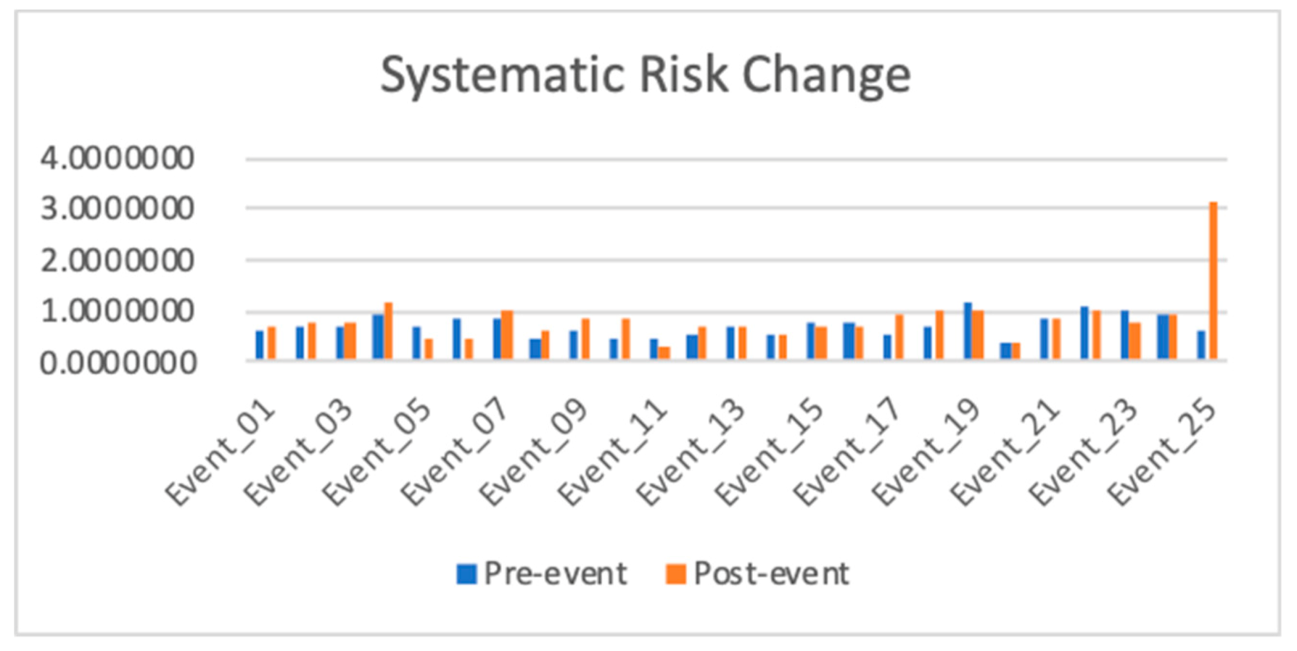
13
Δ(β) = βpost-event − βpre-event.
Figure 1. Maps of occurrence. (a) Geophysical hazards and (b) industrial hazards. Note: The scale of maps represents cumulative observations of event occurrences in each country over the years since 1900.
Jrfm 13 00151 g001
Figure 2. Pre-event and post-event estimations.
Jrfm 13 00151 g002
Table 1. Simple hypothesis testing results.
Cumulative Abnormal Returnt-StatisticsChange of Systematic Riskt-Statistics
Capital Asset Pricing Model (CAPM)−0.694372
(0.4941)
Δ(β)1.312378
(0.2018)
p-values in brackets.

