Clustering of Extremes in Financial Returns: A Study of Developed and Emerging Markets

Abstract

This paper investigates the clustering or dependency of extremes in financial returns by estimating the extremal index value, in which smaller values of the extremal index correspond to more clustering. We apply the interval estimator method to determine the extremal index for a range of threshold values in the developed and emerging markets from 2007–2017. The indices we used to represent developed markets are from France, Germany, Italy, Japan, USA, UK, Spain, and Sweden. For the emerging markets, we use indices from China, Brazil, India, Malaysia, Russia, Saudi Arabia, and Portugal. The results show that clustering occurs in the emerging and developed markets under several threshold values. This study will shed light on the dependency structure of financial returns data and the proprieties of the extremes returns. Moreover, understanding clustering of extremes in these markets can help investors reduce the exposure to extreme financial events, such as the financial crisis.

1. Introduction

The Black–Scholes model assume that financial returns are independent. On the other hand, empirical evidence shows that returns exhibit dependency or long-range dependence (see, Cont 2001; Ding et al. 1993). Furthermore, keeping in mind the diversification of the portfolio where correlation is a crucial factor in the selection criteria, we assume that, in extreme events, investors could also diversify their portfolios by selecting low clustering markets.

Extremes in financial markets are actively discussed because they can have a massive influence on both the economy and the society. This study discusses the property of financial returns and provides insight into the distribution of financial returns data, which is still openly debated in the literature. The aim of this study is to investigates the dependency structure of extreme returns in a variety of stock market indices for developed and emerging markets. Using the interval estimator that was introduced by Ferro and Segers (2003) for a range of threshold values help us better understand the dependency structure of financial returns. In turn, using the estimated extremal index and the dependency structure will shed light on behavior of the financial returns. To our knowledge, a numerical investigation of the clustering extremes behaviour of the developed and emerging stock market indices has not been carried out in the literature; hence we are making preliminary progress in this direction.

The paper is divided into six sections. The next section is a brief literature review. Then, we discuss the methods used to measure clustering. After that, we describe the data used in this study and its limitations. The fifth section present the empirical results, which include a summary table of the main results as well as all the indices’ figures. Then we provide a discussion and we conclude the paper with final remarks and a discussion of future research.

2. Literature Review

It is crucial for investors, regulators, and practitioners to understand the behaviour and statistical proprieties of financial returns data. Some of the common stylised statistical properties of financial returns data as discussed by Cont (2001) include the absence of autocorrelations, heavy tails, the gain or loss of asymmetry, aggregational Gaussianity, intermittency, volatility clustering, conditional heavy tails, slow decay of autocorrelation in absolute returns leverage effect, volume/volatility correlation and asymmetry in time scales. Several studies in the literature have estimated the extremal index in financial return data. For example, Longin (2000) applies the block method estimator to the S&P500 index and finds that θ < 1. Furthermore, Hamidieh et al. (2009) use the interval estimator on crude oil prices, the S&P500 index and Intel’s stock price. The findings are similar to the results obtained by Ferro and Segers (2003). Robert et al. (2009) use the sliding block method and the interval estimator on the negative log returns of the FTSE100 index. Finally, Miranda (2020) applies the block method, run method and found that the interval estimator method produces clear results on the PSI20 index and that θ < 1. Now, we will provide a brief review of the extremal index used with financial returns data. Let ξ₁, ξ₂, … be a sequence of independent identically distributed (IID) random variables (RVs) with distribution function F. Define M_n as the maximum of the first n by:

$$M_n=\max \{{\xi }_1,{\xi }_2,\dots ,{\xi }_n\}.$$

The limiting distribution of maxima in an independent sequence is shown in the following theorem:

Theorem 1.

Let$({\xi }_n)$be a sequence of IID RVs. If there exist constants$a_n>0,b_n\in ℝ$, and some non-degenerate distribution function$G$such that

$$\underset{n\to \infty }{\lim }P(a_n(M_n-b_n)\le x)=G(x)$$

(1)

then,$G$is a generalized extreme value (GEV) distribution.

See, for example, Fisher and Tippett (1928), Leadbetter (1983) and Embrechts et al. (2013). Now, let (ξ_n) be a stationary sequence and M_n be the corresponding maximum values. let, ($\widehat{{\xi }_n}$) be the associated IID sequence and (${\widehat{M}}_n$) the corresponding maximum values. Then, there exists θ ∈ (0, 1] such that

$$\underset{n\to \infty }{\lim }P(a_n({\widehat{M}}_n-b_n)\le x)=G(x)$$

(2)

If and only if

$$\underset{n\to \infty }{\lim }P(a_n(M_n-b_n)\le x)=G^{\theta }(x)$$

(3)

$\theta$ is called the extremal index of the sequence (ξ_n); see Leadbetter (1983). If $\theta$ ≤ 1, then the process suggests clustering. If $\theta$ = 1, the process has no clustering or this is the case of the IID observations. There are several methods used to estimate the extremal index, but the most widely known and used approaches are the blocks estimator and the run estimator. The blocks estimator method is based on the results found by Hsing et al. (1988). The blocks estimator divides the data into p blocks of size q, where n = pq. Then, for each block the maximum is computed as $M_q^{(i)}=\max ({\xi }_{(i-1)q+1},\dots ,{\xi }_{iq})$. By using the following equation, we can then estimate the extremal index.

$${\widehat{\theta }}_n=\frac{{\displaystyle \sum _{i=1}^p{I}_{(M_q^{(i)}>u)}}}{{\displaystyle \sum _{i=1}^n{I}_{({\xi }_i>u)}}}=\frac{B}{N}.$$

(4)

where, I is an indicator function, B is the number of blocks with at least one exceedance of the threshold value u and N is the number of observations that exceed a threshold value u. Robert et al. (2009) showed that better results could be obtained by taking the maxima of the sliding block p = n − q + 1 instead of taking the joint block p = n/q. O’Brien (1987) proposed the run estimator which can be estimated by the following equation

$${\widehat{\theta }}_n=\frac{{\displaystyle \sum _{i=1}^{n-r}{I}_{A_{i,n}}}}{N}.$$

(5)

where, A_i,n = (ξ_i > u, ξ_i+1 ≤ u_n, …, ξ_i+r ≤ u), and N is defined as described before. More details about these methods can be found in the literature by Smith and Weissman (1994) and Embrechts et al. (2013).

These methods require the run length and block size parameters, which may be challenging to estimate. In order to obtain good results, both methods require a large threshold and an optimal choice of block size and run length. Furthermore, studies Ferreira (2018) and Embrechts et al. (2013) summarise and compare the approaches used in estimating the extremal index. We used an approach by Ferro and Segers (2003) (the interval estimator method) that does not require these parameters. Furthermore, Miranda (2020) applied the run, block and interval estimators to financial returns data of the PSI-20 and observed that the difference in terms of bias for the Intervals estimator presents values closer to the runs estimator. However, the region of stability is greater in the intervals estimator. The interval approach is based on the limited result of the number of exceedances threshold and on the convergence of the inter-exceedance times (time between two successive exceedances) of threshold u by the sequence (ξ_n) (see Ferro and Segers 2003; Ferro 2003).

3. Methodology

In our application, we estimated the extremal index value by using the interval estimator method for financial returns data. Define the financial return data as a sequence (ξ_n)_n≥1. Let $N=N_n(u)={\displaystyle {\sum }_{i=1}^{n}I}({\xi }_i>u)$ be the number of returns exceeding threshold u by the sequence (ξ_n). Let 1 ≤ S₁ ≤ … ≤ S_N ≤ n be the observed exceedance times and, T_i = S_i + 1 − S_i be the time between two successive exceedances, where i = 1, …, N − 1. Then, the extremal index θ can be estimated using the following equations:

$${\widehat{\theta }}_n(u)=\frac{2{({\displaystyle {\sum }_{i=1}^{N-1}{T}_i})}^2}{(N-1){\displaystyle {\sum }_{i=1}^{N-1}{T}_i^2}}$$

(6)

$${\widehat{\theta }}_n^{*}(u)=\frac{2{({\displaystyle {\sum }_{i=1}^{N-1}(T_i-1)})}^2}{(N-1){\displaystyle {\sum }_{i=1}^{N-1}(T_i-1)}(T_i-2)}$$

(7)

By combining (6) and (7), we obtain the following equation:

$${\tilde{\theta }}_n(u)=\{\begin{array}{ll}1\wedge {\widehat{\theta }}_n(u)\hfill & \mathrm{if} \max \{T_i:1\le i\le N-1\}\le 2\hfill \\ 1\wedge {\widehat{\theta }}_n^{*}(u)\hfill & \mathrm{if} \max \{T_i:1\le i\le N-1\}>2\hfill \end{array}$$

(8)

${\tilde{\theta }}_n(u)$ is defined as the interval estimator for the extremal index developed by Ferro and Segers (2003). More information on this method can be found in Ferro and Segers (2003) and Ferro (2003). It is worth mentioning that Ferro and Segers’ (2003) interval estimator method is limited in its selection of the optimal threshold value. We compute this value numerically and plot the estimated extremal index values verses the range of threshold values. Since optimal threshold selection is openly discussed in the literature, a common choice for the threshold is to use a high quantile value, which we also use to estimate the extremal index.

We follow the IMF Fund (2017) classification for selecting the countries. There are different financial systems, models, and internal/external factors that should be considered in comparing countries. However, we believe that the stock prices and, consequently the financial returns, will reflect most of these differences in the clustering behaviour.

4. Data1

We explore the dependency structure of extreme returns in a time series of daily logarithmic returns R_n of 16 equity indices from different countries. These indices include both developed and emerging markets. The list of the countries and indices can be found in

Table 1. Country stock indices.

Country	Index Code	Index
Developed economies
France	CAC40	CAC 40 Index
Germany	DAX	DAX Index
Italy	FTSE MIB	FTSE MIB Index
Japan	Nikkei 225	Nikkei 225 Index
USA	S&P500	S&P500 Index
UK	FTSE 100	FTSE 100 Index
Spain	IBEX 35	IBEX 35 Index
Sweden	OMX 30	OMX Stockholm Index
Emerging markets
Brazil	IBOVESPA	Brazil BOVESPA Index
China	SSE	Shanghai Stock Exchange Index
India	BSE SENSEX	Mumbai SENSEX 30 Index
Malaysia	FTSE KLCI	Kuala Lumpur Comp Index
Russia	MICEX	Moscow Interbank Currency Exchange Index
Saudi Arabia	TASI	Tadawul Stock Index
Portugal	PSI20	Portuguese Stock Index

(The countries classification is as the IMF Fund (2017).

. The data are obtained from Trading Economics (2017), and we use the daily log return for the period from 1 July 1997 to 16 January 2017. The average number of observations is (n = 5000). We chose 1 July 1997 as the start of the period because the data for most of the indices in this study are available from 1997 onwards.

The natural asset model that led to the Black–Scholes Model for option pricing is

$$\frac{S_{n+1}-S_n}{S_n}=\mu \delta t+\sigma \sqrt{\delta t}{X}_n,n\in [0,N-1],$$

(9)

Here, $(X_n)$ corresponds to a sequence of IID random variables with $E(X_n)=0$ and unit variance. In the limit $\delta t\to 0$, so that $N\to \infty$ ($T$ fixed), it is shown that the asset prices follow a log-normal distribution:

$$\log (S_T/S_0)~\mathrm{N}\left((\mu -\frac{1}{2}{\sigma }^2)T,{\sigma }^{2}T\right).$$

(10)

Based on the applicability of this model, the extremal index for financial returns data should behave like those of IID observations. In order to meet the assumptions of this model, $\theta$ should be equal to 1 since no clustering appear for IID data. In our analysis $R_n=log\frac{S_n}{S_{n-1}}$, and we analyse the dependency or clustering of the maximum financial returns as $M_n=\max \{R_1,R_2,\dots ,R_n\}.$

5. Results

In this section, we examine the extremal index for all the indices at different threshold values as illustrated in Figure 1, Figure 2, Figure 3, Figure 4 and Figure 5. The results show a stable region of the plot of $\theta \approx 0.3$. An accurate result of $\theta$ depends on the choice of the optimal threshold value. Arguably, a natural choice of the threshold value is a high quantile. Furthermore, we present an empirical results obtained by estimating the extremal index for daily financial returns in developed and emerging markets, as presented in

Table 2. The estimated extremal index θ for developed and emerging markets.

Country	Index	0.95		0.99
		u	θ	u	θ
Developed economies
France	CAC40	0.0222	0.4304	0.0387	0.2878
Germany	DAX	0.0237	0.3011	0.0398	0.3434
Italy	FTSE MIB	0.0242	0.1137	0.0389	0.2709
Japan	Nikkei 225	0.0234	0.4481	0.0386	0.2938
USA	S&P500	0.0180	0.2975	0.0347	0.2770
UK	FTSE 100	0.0183	0.3519	0.0313	0.2835
Spain	IBEX 35	0.0233	0.3553	0.0380	0.3037
Sweden	OMX 30	0.0240	0.2532	0.0416	0.3315
Emerging markets
Brazil	IBOVESPA	0.0302	0.4631	0.0517	0.1939
China	SSE	0.0249	0.4544	0.0421	0.4484
India	BSE SENSEX	0.0239	0.3884	0.0391	0.3994
Malaysia	FTSE KLCI	0.0104	0.2750	0.0337	0.1271
Russia	MICEX	0.0352	0.2933	0.0692	0.2897
Saudi Arabia	TASI	0.0185	0.3794	0.0366	0.3344
Portugal	PSI20	0.0185	0.2303	0.0299	0.3553

.

We found that all the indicess’ extremes show clustering for the corresponding extremal index value $\theta \le 1$ of all sample countries with large threshold values. Moreover, using the 0.99 quantile of the indices of the S&P500, FTSE100, CAC40, MICEX markets result in $\theta \approx 0.28$. Notably, the results show that, even though it is an emerging market, China has lower clustering when compared to the developed economies in the sample. Finally, both Brazil and Malaysia show higher clustering than developed economies, which is expected as they are emerging markets.

6. Discussion

The empirical results in this study suggest that for the overall the values of the extremal index in all indices $\theta$ ≤ 0.46. This for the 0.95 and 0.99 quantiles, as seen in Miranda (2020), Hamidieh et al. (2009), Robert et al. (2009) and Alokley (2015). The results show that, for developed countries, $\theta$ > 0.25; this indicates clustering for the 0.99 threshold. Our result of the S&P500 is in agreement with Hamidieh et al. (2009), who estimated the extremal index and found that $\theta$ = 0.33 with 95% confidence by using the Maxspectrum and Ferro–Segers estimates. Furthermore, Alokley (2015) estimates a close result. However, Longin (2000) investigate the stock market returns of the S&P500 using the blocks method and find that $\theta$ = 0.72 was minimal for one-day returns. Moreover, our results for the FTSE100 are 0.35, 0.28 for the 0.95 and 0.99, respectively. These results are close to the results of Robert et al. (2009), who investigated the FTSE100 index and found that $\theta$ = 0.33. 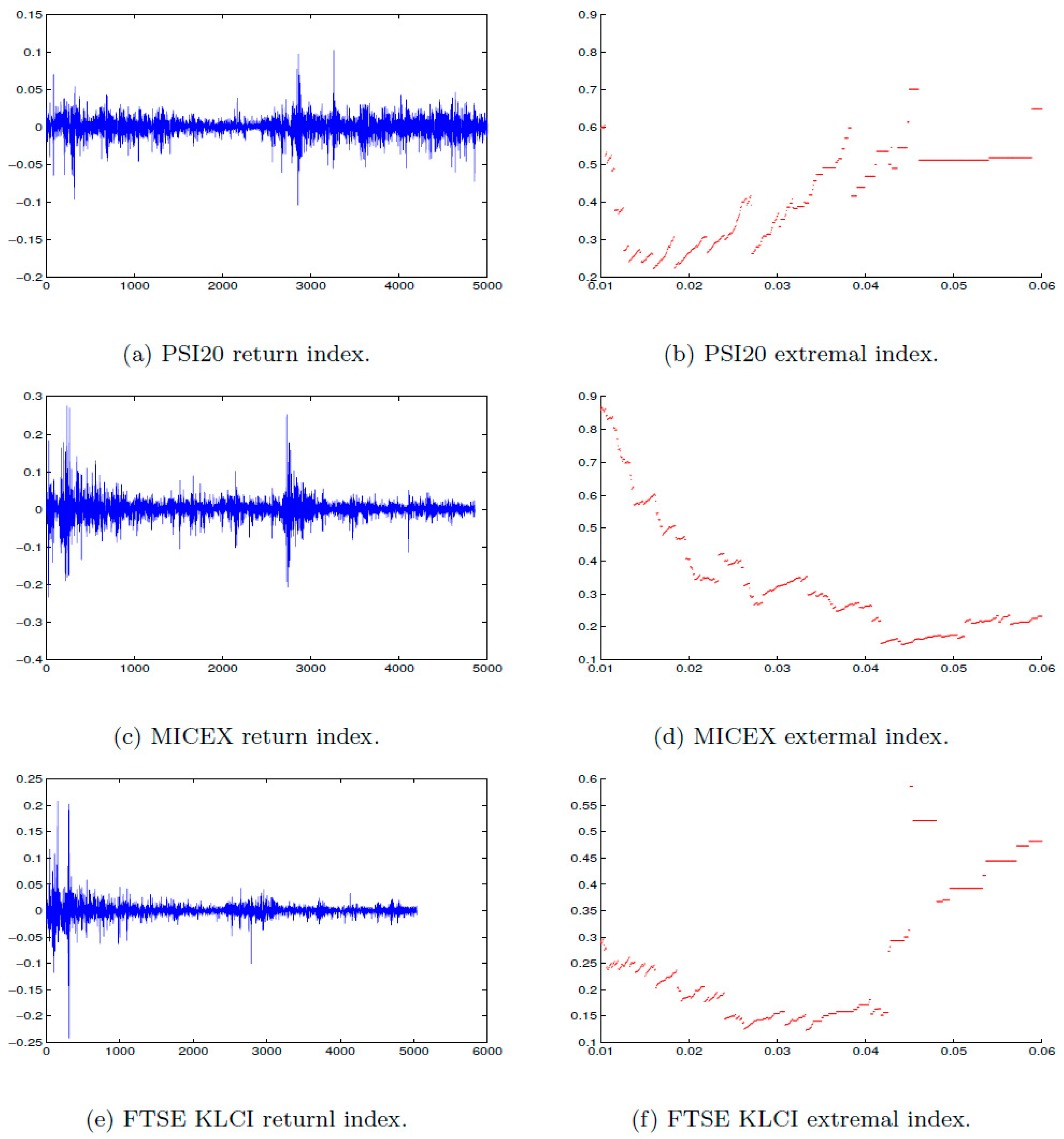Both results agree with Alokley (2015) findings. Furthermore, our findings for the PSI20 show a stable region of $\theta$ values from 0.2 to 0.3, as shown in Figure 5b; this result is in agreement with Miranda (2020).

Furthermore, as expected, the degree of clustring is higher, on average, for emerging markets, especially FTSE KLCA and IBOVESVA. Overall, the IBOVESPA Index (Brazil Stock Market) and the FTSE KLCI Index (Malaysian Stock Market) show more clustering with a 0.99 quantile. To our knowledge, no previous study has investigated the clustering of emerging markets; hence our results may shed light on the behaviour of clustring in these markets. Our findings also show that most of the indices in the emerging markets behave similarly to the developed markets. The final result that is relevant to our financial application is the following: the exceedances of the high threshold for financial return data in all the countries exhibit clustering and do not behave as IID data. Therefore, the Black–Scholes model does not apply to financial return data.

Authors should discuss the results and how they can be interpreted in perspective of previous studies and of the working hypotheses. The findings and their implications should be discussed in the broadest context possible. Future research directions may also be highlighted.

7. Conclusions

In this paper, we attempt to better understand the behaviour of financial returns data in developed and emerging markets. Empirical results suggest that the degree of clustering in stock market returns is high for both emerging and developed economies. Selecting low clustering markets can be help to overcome extreme financial events. It is also worth mentioning that the results depend on the threshold value used to estimate $\theta$. Our results’ limitations are mainly related to the optimal threshold value, since this study used a range of thresholds in the pursuit of accurate and dependable findings.

Future research can explore the following areas: (1) It might be of interest to determine which financial model could explain this empirical behavior since no clustering occurs for IID data. (2) An investigation could be carried out to better understand the clustering of volatility. (3) It is also useful to apply this method to investigate the behaviour of the oil markets returns. Estimating an accurate as a measure of clustering will help investors and portfolio managers diversify their portfolios, and will also help policymakers to regulate financial markets.

References

- Alokley, Sara Ali. 2015. Understanding Extremes and Clustering in Chaotic Maps and Financial Returns Data. Ph.D. thesis, University of Exeter, Exeter, UK. [Google Scholar]
- Cont, Rama. 2001. Empirical properties of asset returns: Stylized facts and statistical issues. Quantitative Finance 1: 223–36. [Google Scholar] [CrossRef]
- Ding, Zhuanxin, Clive W. J. Granger, and Robert F. Engle. 1993. A long memory property of stock market returns and a new model. Journal of Empirical Finance 1: 83–106. [Google Scholar] [CrossRef]
- Embrechts, Paul, Claudia Klüppelberg, and Thomas Mikosch. 2013. Modelling Extremal Events: For Insurance and Finance. Berlin: Springer Science & Business Media, vol. 33. [Google Scholar]
- Ferreira, Marta Susana. 2018. Heuristic tools for the estimation of the extremal index: A comparison of methods. REVSTAT 16: 115–36. [Google Scholar]
- Ferro, Christopher A. T. 2003. Statistical Methods for Cluster of Extreme Values. Ph.D. thesis, University of Lancaster, Lancaster, UK. [Google Scholar]
- Ferro, Christopher A. T., and Johan Segers. 2003. Inference for clusters of extreme values. Journal of the Royal Statistical Society: Series B (Statistical Methodology) 65: 545–56. [Google Scholar] [CrossRef]
- Fisher, Ronald Aylmer, and Leonard Henry Caleb Tippett. 1928. Limiting forms of the frequency distribution of the largest or smallest member of a sample. Mathematical Proceedings of the Cambridge Philosophical Society 24: 180–90. [Google Scholar] [CrossRef]
- Hamidieh, Kamal, Stilian Stoev, and George Michailidis. 2009. On the estimation of the extremal index based on scaling and resampling. Journal of Computational and Graphical Statistics 18: 731–55. [Google Scholar] [CrossRef]
- Hsing, Tailen, Jürg Hüsler, and Malcolm Ross Leadbetter. 1988. On the exceedance point process for a stationary sequence. Probability Theory and Related Fields 78: 97–112. [Google Scholar] [CrossRef]
- IMF Fund. 2017. World Economic Outlook Data, April 2017 ed. Washington: IMF Fund. [Google Scholar]
- Leadbetter, M. Ross. 1983. Extremes and local dependence in stationary sequences. Zeitschrift für Wahrscheinlichkeitstheorie und Verwandte Gebiete 65: 291–306. [Google Scholar] [CrossRef]
- Longin, Francois M. 2000. From value at risk to stress testing: The extreme value approach. Journal of Banking & Finance 24: 1097–130. [Google Scholar]
- Miranda, Maria Cristina Souto. 2020. Extremal index estimation: Application to financial data. In Handbook of Research on Accounting and Financial Studies. Hershey: IGI Global, pp. 96–130. [Google Scholar]
- O’Brien, George L. 1987. Extreme values for stationary and markov sequences. The Annals of Probability 15: 281–91. [Google Scholar] [CrossRef]
- Robert, Christian Y., Johan Segers, and Christopher A. T. Ferro. 2009. A sliding blocks estimator for the extremal index. Electronic Journal of Statistics 3: 993–1020. [Google Scholar] [CrossRef]
- Smith, Richard L., and Ishay Weissman. 1994. Estimating the extremal index. Journal of the Royal Statistical Society. Series B (Methodological) 56: 515–28. [Google Scholar] [CrossRef]
- Trading Economics. 2017. Index Daily Closing. Available online: Tradingeconomics.com (accessed on 16 January 2017).