Abstract
We provide an innovative methodological contribution to the measurement of returns on infrequently traded assets using a novel approach to repeat-sales regression estimation. The model for price indices we propose allows for correlation with other markets, typically with higher liquidity and high frequency trading. Using the new econometric approach, we propose a monthly art market index, as well as sub-indices for impressionist, modern, post-war, and contemporary paintings based on repeated sales at a monthly frequency. The correlations enable us to update the art index via observed transactions in other markets that have a link with the art market.
JEL Classification:
C14; C43; Z11
1. Introduction
The recent financial crises caused by the Lehman bankruptcy and the European sovereign debt problems have increased the interest in safe haven investments. Standard safe haven investments having either no protection against inflation (in the case of bonds) or high volatility (such as gold), investors may have been attracted by alternative assets such as real estate, fine art, or wine. The development of the fine art funds confirms that investors view artworks as just another asset class of investment. This growth was fueled by many factors, including a search by investors for higher yields, and entrance into the market of Chinese and emerging markets collectors who are diversifying their acquisitions and investing in art. Practitioners in the field of art-finance require tools to track the evolution of prices in the art market. For instance, regulated funds must be able to refresh regularly their net asset value for regulatory purposes, as well as to serve redemptions at fair value to their investors. Insurers equally face challenges to re-assess the insured value of art regularly while a growing industry of art loans relies on regular valuations to assess their exposure to the art market. According to Deloitte Picinati di Torcello (2012), the outstanding value of artworks exceeds three trillion dollars globally. The Observer Grant (2018) reported that hurricane Sandy cost approximately half a billion dollars in damage to artworks in private home and commercial galleries. Regularly tracking movements in the art market is essential for insurers and brokers to manage their market risks properly and re-evaluate insurance premia to their clients. The evaluation of these markets on a higher frequency time scale such as monthly is hampered by the heterogeneity of goods and illiquidity caused by periods of few if any transactions. Nonetheless, a reliable high frequency evaluation is important for valuation, optimal investment allocation, risk management, and the understanding of correlation and spill-overs from and to other markets. Furthermore, new high frequency re-valuation approaches other than traditional art expertise could help further grow the art fund industry by increasing the transparency of methodologies for mark-to-market accounting. In particular, practitioners active in derivatives markets (known as “price guarantees”) could benefit from more accurate estimates of market returns at higher frequencies. The purpose of this paper is to introduce a new approach to the construction of monthly art indices. So far, the literature addressed mostly the heterogeneity issue. Two estimation methods are commonly used to construct indices: (1) repeat-sales regression (RSR) and (2) hedonic regression (HR).
RSR uses prices of individual objects traded at two distinct moments in time. If the characteristics of an object do not change (which is usually the case for collectibles), the heterogeneity issue is bypassed. Goetzmann (1993) constructed a decennial repeated sales index, using 2809 artworks re-sold at auction from the Gerald Reitlinger and Enrique Mayer databases over a period covering 1715 to 1986. Mei and Moses (2002) constructed a repeated-sales dataset based on auction art price records at the New York Public Library, as well as the Watson Library at the Metropolitan Museum of Art with a total of 4896 price pairs covering the period 1875–2000. They constructed an annual art index to study the risk-return characteristics of paintings, which they found compared favorably to those of traditional financial assets, such as stocks and bonds.
The basic idea of the HR method is to regress prices on various attributes of objects (dimensions, artist, subject matter, etc.) and to use time dummies in the regression to obtain “characteristic-free” prices to compute a price index.1
The main advantage of RSR, compared to HR, is that the estimation of the returns does not require the inclusion of explanatory variables in the model. The main disadvantage of the repeated-sales methodology is the less frequent occurrence of resales pairs, whereas the HR typically takes advantage of all available observations. RSR is therefore not efficient in a statistical sense, as it discards many observations. On the other hand, it has the advantage—compared to HR—that it is not prone to model specification error through variable selection. Ginsburgh et al. (2006) provided a detailed comparison of RSR and HR, including a Monte Carlo study, and concluded that in large samples, both approaches provided very similar results. In our application, the sample is sufficiently large even at the monthly frequency, so that the inefficiency of RSR should be negligible. In addition, one of the novelties in this paper is that we augment the standard RSR regression by a filter, which (a) extracts an unobserved index and (b) reduces the standard errors of classical RSR. The latter further improves the efficiency of RSR. Korteweg et al. (2016) considered repeat-sales as endogenous by including a hazard model for the probability of a sale. They constructed an annual index using 32,928 transactions over the period 1960 to 2013. This methodology required a closed model to estimate the likelihood of selling an artwork based on its characteristics. Unfortunately, such a method is impractical in absence of data on unsold artworks and their corresponding explanatory variables, or in case the data sample is too small to estimate dynamic variables of the selection correction properly. Our methodology focuses on high frequency (month-to-month) sparse data with little or incomplete information, as is usually the case in the art market.
We provide an innovative methodological contribution to the measurement of returns on infrequently traded assets using a novel approach to repeat-sales regression estimation. Using the new econometric approach, we propose a monthly art market index, as well as sub-indices for impressionist, modern, post-war, and contemporary paintings based on repeated sales at a monthly frequency. Our starting point is a model proposed by Bocart and Hafner (2015). We address the question by extending a recently proposed dynamic state space model—inspired by Aruoba et al. (2009)—for price indices of heterogeneous goods to allow for correlation with other markets, typically with higher liquidity and high frequency trading. Ignoring correlation would lead to flat indices in times of no transactions, as is common in the art markets due to the strong biannual cycle of auctions. A precise estimation of correlation enables us to update the art index via observed transactions in other markets that have a link with the art market. In statistical terms, this improves the efficiency of estimated price indices.
In particular, the construction of the monthly index exploits links of art with other assets available at higher frequencies such as liquid exchange traded funds focusing on consumer goods or real estate, baskets of art-related companies (Sotheby’s, artnet, artprice, etc.) or furniture companies, and safe haven assets like gold or U.S. Treasuries.
The paper is organized as follows. In Section 2, we present the econometric model specification and estimation. Empirical findings for the five price indices: impressionist art, modern art, post-war art, contemporary art, and finally, a global art market index are reported in Section 3. In Section 4, we study art as an asset class and report standard asset pricing model estimates for the various art market indices. A final section concludes the paper.
2. Model Specification and Estimation
Our objective is to construct a monthly art index from repeated sales, which are observed on an irregular time scale. Let denote the log price of an artwork i sold at time t, with N denoting the total number of artworks in the sample. The repeated sales methodology requires that each artwork i has been traded at least twice over the sample period, otherwise it is excluded from the sample. At date t, let be the total number of transactions, which may be zero, so that . The transactions are collected in the vector , where missing observations are skipped, so that is of dimension (). In addition to these prices, we observe , a K-vector of observed prices of traded assets that are related to the art market, or other quantitative information that is presumed to be related. For example, could contain the price of a basket of stocks listed on a stock exchange whose constituents have business in the art market (e.g., Sotheby’s, artnet, artprice, etc.), or say the price of gold or other precious metal. In general, will be non-stationary, e.g., a random walk in the case of stock prices. For our purposes, we transform to obtain a stationary sequence , e.g., taking log-returns.
2.1. Model Specification
The model consists of the following system of equations:
Equation (1) is similar to the models of Bailey et al. (1963) or Goetzmann (1992) used to estimate real estate returns from repeated sales. Both are special cases of Case and Shiller (1987).2 The coefficients are fixed effects, specific for each artwork, and invariant over time. The evolution of the market index is determined by the latent process , which, as specified in Equation (2), evolves as a random walk with drift. The system of Equations (1) and (2) is essentially a dynamic panel model with random nonstationary time effects and fixed painting-specific effects . The panel is unbalanced because missing observations are discarded from Equation (1). Note that, while is a random walk with drift, which is made clear in the second equation, is mean zero as is stated in the last equation. In our empirical application, we will set , so that + is a mean zero non-stationary process.
Without Equation (3), or equivalently with , this model would be a classical repeated sales model. A non-zero covariance links the price Equation (1) for artworks to that of observed asset returns in (3). These observed returns have conditional expectation , parameterized by a p-vector , where denotes the information set generated by lagged and up to time . That is, could follow, e.g., an ARMA-type process, perhaps including lags of observed art returns.
The error covariance structure imposes zero correlation between the idiosyncratic errors of the repeated sales regression and the remaining error terms. The novelty is the assumption of a potential correlation between the error term of the art market, , and the error terms of the observed assets, . This will allow the filter to update the index taking into account the observations .
While the complete covariance matrix has dimension , it should be noted that the matrix features many zero restrictions. In particular, the upper left sub-matrix is diagonal with a single parameter governing the homoskedastic errors. In addition, the lack of correlation between those innovations and respectively and imposes another zero restriction. Hence, we are left with a -dimensional sub-matrix of parameters to estimate, with K relatively small.
2.2. Estimation
To estimate the model, we propose a maximum likelihood estimator combined with the Kalman filter to recover the underlying state variables. Without further constraints, the parameters in the term are not jointly identified. A common practice in repeated sales is to take “first differences”, i.e., returns, that eliminate the asset specific effects . An equivalent approach is to impose that has a mean of zero and to estimate as the average of transaction prices of asset i. We follow the second approach and obtain estimates of and of the composite error term . Then, the model (1) permits the following linear Gaussian state space representation:
for = where , , and are vectors of length .3 Furthermore, let , a vector of length . We denote the following conditional distributions,
For a given set of parameters, the conditional means and variances can be obtained using the following Kalman recursions:
- Prediction step ():
- Correction step ():
- Smoothing step ():To estimate the underlying state , one uses the full sample information ().
The second term on the right-hand side of the updating equation for in (12) would not depend on current transactions if were zero, because then , and its inverse would be block-diagonal. With ≠ however, the updating of will depend on this correlation, and on the prediction error of returns . The above steps assume that , so that at each time t, we have at least one transaction in the art market. For the case where , we use a fictitious art transaction whose log price corresponds exactly to its prediction 4. This ensures that, in times of no activity in the art market, the market index is still updated via the second term in (12).
Parameter estimation can be achieved in an efficient and straightforward way by maximum likelihood. Denote the parameter vector by and corresponding parameter space , which is -dimensional. Let and . Then, the log-likelihood, up to an additive constant, can be written as:
and the maximum likelihood estimator is defined as:
The maximization problem has no analytical solution, but numerical methods can be used conveniently.
Simplifications are possible by assuming that , so that the conditional mean of only depends on its own history. In that case, one can estimate and separately in a first step. In the second step, the dimension of reduces to . One has to impose restrictions on that keep positive definite, but this is easier to achieve than a simultaneous estimation of if K is large.
The model allows for yet further improvements that go beyond the scope of our current application: for instance, a known drawback of the repeated sales methodology applied to the art market is the potential presence of a sample selection bias. Collectors could re-sell artworks at auction conditional to the fact that their price increased in value. Similarly, artworks that fell out of fashion may never be sold again given lack of demand for a specific artistic style. These sample selection effects tend to bias return estimates positively. However, to the contrary, master artworks acquired by museums may never be re-sold, and paintings with large price appreciations may be sold privately, leading to a negative bias of indices based on auction data. All in all, using ordinary least squares estimates, Ginsburgh et al. (2006) found that in the art market, when the sample is large and over a large period of time (typically 20 years), both methodologies converge towards the same estimated returns. Zanola (2007) introduced a selection corrected repeat-sales index based on the two-step procedures of Heckman (1974), which could be included in the state equation.
Other improvements to the state equation can naturally be the introduction of more explanatory variables or auto-regressive components in view of mitigating index revision. Revision is the deviation in estimates each time new data are included in the sample. In particular, van de Minne et al. (2019) pointed out that a structural time series repeat-sales model including an autoregressive process can help mitigate revision for real estate indices, as well as the inclusion of sector-wise explanatory variables. Simulated data offer an insight into the robustness of the methodology with respect to revision: a simulation of transactions behavior at auction shows that revision could change estimated overall returns by up to +5% between a 10 year and a 20 year estimate.
3. Empirical Findings
Our goal was to compute five price indices. Four of them correspond to the most important periods of recent art history: impressionist art, modern art, post-war art, and contemporary art. A fifth index was built, merging all movements into a global art market index. For each category, we selected the 50 artists that exhibited the largest monetary volumes of paintings sold at auction between January 2002 and September 2017. Art data and categorization of artists by movements are provided by artnet A.G. These 200 artists represented 49,641 lots sold at auction for a total amount of $43.9 billion. Exactly 3059 artworks by these artists were sold at multiple intervals between January 2002 and September 2017, for a total of $6.9 billion in repeated sales. Prices included the buyer’s premium, i.e., transaction costs.
To help estimate the evolution of prices of each art category, several liquid assets were selected: the S&P 500 index, the iShares U.S. consumer goods ETF, the iShares U.S. real estate ETF, the iShares 20 years Treasury ETF, the spot price of the gold bullion, the West Texas Intermediate spot price, an equally-weighted basket of art-related companies consisting of Sotheby’s, artnet A.G., artprice S.A., and Collector Universe Inc., an equally-weighted basket of furniture-related companies.5 Finally, we also constructed an equally-weighted basket of the following luxury companies: Dior S.A., Moët Hennessy Louis Vuitton SE, and Kering. All data were provided by Yahoo! Finance, except the Gold Fixing Price in London Bullion Market in USD and the West Texas Intermediate spot price, which were provided by the Federal Reserve Bank of St. Louis.
As discussed in the previous section, the index was computed in two steps. First, the conditional means of financial asset returns were separately estimated as the six month moving average of log price returns for each of the listed assets. This also gave an estimator of , the variance-covariance matrix of the error term . The painting-specific effects were estimated as the average log transaction prices of each painting. In a second step, the parameters of the Kalman filter were estimated via maximum likelihood, where we set the drift of the random walk to zero for simplicity. To highlight the advantages of the RSR methodology compared with a hedonic approach, a hedonic version of the global index using the same data was constructed using the methodology of Bocart and Hafner (2015). Figure 1 shows that such a hedonic-based model leaf much more unnatural variance in the index that was likely tied to the strong heterogeneity of data and the impossibility to reconcile this into a single linear explanatory model.
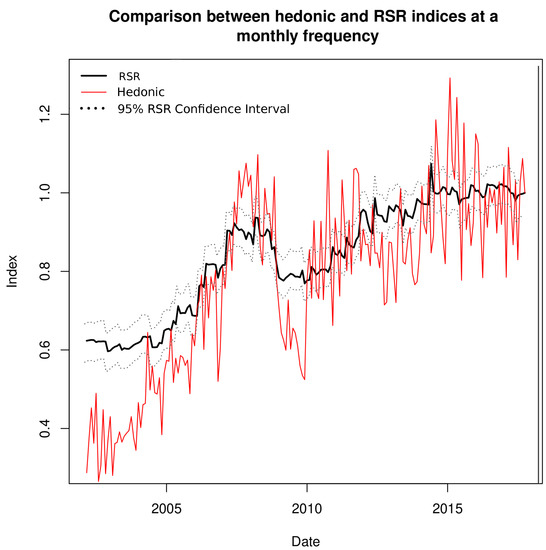
Figure 1.
Kalman-repeat-sales regression (RSR) vs. Kalman-hedonic.
Figure 2 illustrates the five price indices: impressionist art, modern art, post-war art, and contemporary art and the solid line representing the global art market index. Overall, we observed a rise of the indices up until the recent financial crisis. Starting roughly in 2009, we also observed for the global art index, as well as some of the sub-indices an upward trend. Notable exceptions were the impressionist art index and to a certain degree modern art as well, which were mostly flat since the financial crisis. In contrast, we noted a strong performance of both the contemporary and post-war indices.
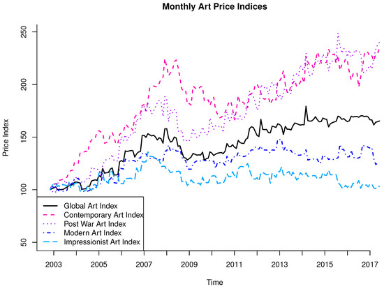
Figure 2.
Art indices.
Since the inclusion of financial market information was relevant only in the case of non-zero correlation, we proceeded to maintain candidates that exhibited a correlation of at least 10% in absolute value between their monthly log-returns and the art index’s monthly log-returns.6 The empirical results appear in the middle panel of Table 1.

Table 1.
Returns, volatility, and correlation of the price indices.
Out of the different assets selected, only a few exhibited a correlation with art: S&P 500, art companies, real estate ETF, and luxury companies exhibited a positive correlation in their returns with those of the global art index, ranging from 12% for luxury companies to 25% for the basket of art-related companies. Gold returns on the other hand were negatively correlated with returns of the global art index. As expected, all art movements positively correlated with the monthly stock returns of art companies.
Monthly returns of the contemporary art index seemed to correlate negatively with those of luxury companies (−14%), a result a priori counter-intuitive since one would expect luxury contemporary art to correlate positively with the performance of luxury companies. A possible explanation would be the substitution effect between different types of luxury goods, highlighting a switch in demand for luxury goods sold in shops and galleries to the ones sold at second hand auctions.
Monthly returns of post-war art correlated with those of the S&P 500, but also with furniture companies, a sign that prices of artworks by artists like Andy Warhol and Roy Lichtenstein may benefit from increased spending in interior decoration. Modern art returns presented a positive correlation with real estate ETF returns, indicating a comovement between blue chip Modern artists such as Pablo Picasso or Joan Miro and the real estate sector. A few asset classes did not exhibit any form of correlation with any of the art movements: returns of the iShares U.S. consumer goods ETF, the West Texas Intermediate (oil price), and U.S. Treasury bonds did not comove with those of artworks. Impressionist art, which correlated positively with art companies, had the lowest Sharpe ratio (0.02) given an annualized return close to zero for a volatility (12%) similar to contemporary art (11%) or the S&P 500 (14%).
The lower panel of Table 1 displays the correlations among the different art indices. The global index correlated most with post-war and modern. Correlations among the sub-indices were at most 27%, namely between post-war and modern.
In Table 2, we report the correlation of the global art index with the 49 industry portfolios retrieved from the Ken French web page. We report results for three samples. Besides the full sample, we report a pre-crisis sample, which ended in August 2008, and a post-crisis sample starting in September 2008 and ending in September 2017. The industries were ranked from high correlations to low, using the full sample results. We observed that the top of the list was the beer and liquor industry with a correlation of roughly 27%. The other toppers were quite heterogeneous. This included banking and trading, but also “other”, which stands for anything not listed in the 48 other industries, rubber and plastic, candy and soda, retail, personal services, business supplies and services. The pre-crisis sample featured smaller correlations, whereas the opposite was the case for the post-crisis sample. In fact, the highest correlation for the latter was again beer and liquor and reached 35%. The tail end of the list was the precious metals industry with a large negative correlation of 25% in the pre-crisis sample. This finding related to the earlier reported correlation of the art indices with gold. In the Appendix A, we also provide results pertaining to the 49 industry correlations and the sub-indices; see Table A2, Table A3, Table A4 and Table A5. Overall, the findings were similar for all but the contemporary art index, except that typically, the correlations were lower than those for the global art index. The contemporary art index appearing in Table A5 showed a correlation ranking that was quite different. The top industry in the full sample was fabricated products for example; although, that correlation was only 13%. Finally, almost a third of the industries featured negative correlations with the contemporary art index.
Table 2.
The table reports the Pearson correlation between the global art index and each of the Fama and French 49 industry groups over three time periods. Full sample refers to correlations computed using monthly data ranging from 2002:04 to 2017:09; pre-crisis correlations are computed using data ranging from 2002:04 to 2008:08; and post-crisis correlations are computed using data ranging from 2008:09 to 2017:09.
4. Art as an Asset Class
Having art market indices at the monthly frequency brought us in line with the more traditional asset pricing literature. A number of studies have analyzed the infrequently observed auction-based price series. Initial studies include Stein (1977), Baumol (1986), Goetzmann (1993), Buelens and Ginsburgh (1993), Pesando (1993), Chanel (1995), Mei and Moses (2002 and 2005), among others. Anderson (1974) concluded, using data for the period 1643–1970, that paintings had offered a return that was about fifty percent lower than the return offered by common stocks. Using U.S. and U.K. auction prices for paintings sold between 1946 and 1968, Stein (1977) found a nominal return of 10.5% compared to an annual nominal return on stocks of 14.3% for the same period, whereas Baumol (1986), based on records from 640 painting transactions between 1652 and 1961, found that paintings had a lower return when compared to that of risk-free assets. More recently, Renneboog and Spaenjers (2013), using data covering the period 1957–2007, built an art index that exhibited a modest 3.97% real annual return expressed in U.S. dollars; that is, a performance similar to that of corporate bonds, but with much higher risk. Mandel (2009) also found similar results for the period 1950–1999, namely that art exhibited returns lower than both the S&P 500 and the Dow Jones industrial index, but with higher volatility.
A traditional explanation for lower returns of art compared to other assets is the “aesthetic dividend”, described by Baumol (1986) and Mandel (2009). The aesthetic dividend theory states that lower returns are compensated by higher utility of holding the work: art collectors enjoy the piece and benefit from the social status associated with art ownership. However, the implied aesthetic dividend differs greatly between contemporary art (+6% average annualized return) and modern art (+2% average annualized return) or impressionist art (0% average annualized return). It appears that older art movements lead to lower short-term returns. Arguably, artworks distributing the highest aesthetic dividend should also be the ones in higher demand for their aesthetic characteristics. It is expected that these works in high demand would also exhibit higher liquidity at auction. As a consequence, one should observe lower bought-in rates 7 for these older artworks. However, the opposite was observed: it seemed that not only contemporary art outperformed its peers in terms of returns, but it was also more successful at auction in the period 2003–2017, with only 20% of lots failing to sell compared to 25% for modern artists or 26% for impressionist masters. This contradiction cannot be easily reconciled with the notion of aesthetic dividend that suggests artworks have low returns when they are highly desirable. One could conjecture that another mechanism is behind these lower returns for older artists: these more established artists, like Renoir, Manet, or Gauguin, though less fashionable8, have a proven track record of surviving trends and fashion cycles throughout history. Established masters may offer more guarantees of a future resale, on time horizons untested by the scope of our dataset. In a nutshell, it can be conjectured that a basket of contemporary artists in the 21st Century may be more risky to hold over long periods of time than a basket of established impressionist or modern artists. In other words, even though the volatility of short-term returns may be similar between impressionism and contemporary art, liquidity risks borne by art investors on much lower time frequencies (typically, decades or even centuries) could justify lower short-term returns. This hypothesis was supported by Vermeylen et al. (2013), who tracked canon formation for Flemish and Dutch painters from the 17th Century. The authors highlighted the high volatility in market preferences through time. They observed that many artists believed to be contemporary canons at different periods “fell through the cracks of history”.
Buelens and Ginsburgh (1993) used a hedonic regression approach and found the conclusions of Baumol overly pessimistic. In a similar vein, Goetzmann (1993) found that paintings’ investment had an annual appreciation of 17.5% between 1900 and 1986, while the London Stock Exchange index had a return of merely 4.9% over the same period. Likewise, Mei and Moses (2002) reported that the returns on art works were higher than returns on fixed-income assets and equivalent to returns on equities, while featuring higher volatility. Renneboog and Spaenjers (2013) provided a comprehensive literature review regarding art returns. Using a hedonic price index based on 1.1 million auction transactions, they found that art had a lower Sharpe ratio than equities. Oosterlinck (2016) found that art outperformed all other asset classes in occupied Paris in 1940–1944, suggesting that art may be a good hedge against low probability disasters.
The above discussion highlights the fact that there as a wide range of results, many contradictory, regarding the performance of art as an asset class. However, a somewhat uniform verdict emerged from the literature: art returns associated with paintings did not appear attractive when compared with stocks and bonds.
Our new indices allowed us to shed new light on the asset pricing implications of art holdings. We started with the top panel of Table 1. We note that the annualized returns of the art indices were all below the 8% for the S&P 500 over the full sample. The best returns were obtained with contemporary and post-war art. The most dismal performance was impressionist art. In terms of volatility and the Sharpe ratio, we note that contemporary art appeared to perform almost as well as the S&P 500. Nevertheless, art and luxury goods companies showed better performance numbers that any of the art indices. Interestingly, real estate was not as attractive as contemporary and post-war art when one compares their Sharpe ratios.
Next, we turn our attention to Table 3 in which CAPM parameter estimates are reported for the full sample, as well as the pre- and post-crisis subsamples. The results showed that the beta estimates were low, most between 0.10 and 0.15. The impressionist art index featured a negative beta, except post-crisis. The most remarkable result was the contemporary art index. In the full sample, it had a zero beta and an alpha of 0.38, implying about a 4.5% annual return. However, in the pre-crisis sample, the alpha increased to almost one, or a 12% annual return, with a slightly negative beta. This looked more like the performance of a respectable hedge fund. In the post-crisis sample, this stellar performance totally disappeared however. Table 4 and Table 5 paint a similar picture. They report time-series regressions of the monthly returns associated with each art index on respectively three factors of the Fama and French (1993) (Table 4) and the same three factors augmented with the momentum factor (UMD) of Carhart (1997) and the liquidity factor (PS) of Pástor and Stambaugh (2003). Note that these results implied that the art market index returns could not be explained by standard equity momentum or liquidity risk factors.
Table 3.
The table reports the results of time-series regressions of the monthly returns associated with each art index on the excess returns of the value-weighted market portfolio (MKTRF). is expressed as a percentage per month, and Newey–West t-statistics are reported in parentheses. Note that returns for the contemporary art index begin in 2002:07.
Table 4.
The table reports the results of time-series regressions of the monthly returns associated with each art index on the three factors of Fama and French (1993). is expressed as a percentage per month, and Newey–West t-statistics are reported in parentheses. Note that returns for the contemporary art index begin in 2002:07.
Table 5.
The table reports the results of time-series regressions of the monthly returns associated with each art index on the three factors of Fama and French (1993) augmented with the momentum factor (UMD) of Carhart (1997) and the liquidity factor (PS) of Pástor and Stambaugh (2003). is expressed as a percentage per month, and Newey–West t-statistics are reported in parentheses. Note that returns for the contemporary art index begin in 2002:07.
5. Conclusions
We provided an innovative methodological contribution to the measurement of returns on infrequently traded assets using a novel approach to repeat-sales regression estimation. Our starting point was a model proposed by Bocart and Hafner (2015). We addressed the question by extending a recently proposed dynamic state space model—inspired by Aruoba et al. (2009)—for price indices of heterogeneous goods to allow for correlation with other markets, typically with higher liquidity and high frequency trading.
Leaving the artistic and aesthetic value of paintings aside, there is a growing interest in the investment value of art. The new econometric methodology allowed us to estimate a monthly art market index, as well as sub-indices for impressionist, modern, post-war, and contemporary paintings based on repeated sales at a monthly frequency.
In terms of volatility and the Sharpe ratio, we found that contemporary art appeared to perform almost as well as the S&P 500. Nevertheless, art and luxury goods companies showed better performance numbers than any of the art indices. Interestingly, real estate was not as attractive as contemporary and post-war art when one looks at their Sharpe ratios. The most remarkable result was the contemporary art market index. In a sample up to the financial crisis, the alpha and beta of the index featured the performance of a respectable hedge fund. None of the art index returns loaded significantly on momentum or liquidity factors, let alone the Fama–French factors.
The methodology proposed in the current paper has many other applications in markets with features similar to those of the art market; in particular, markets where trading occurs infrequently during periodically scheduled auctions and one observes frequently traded related assets. Examples include wine, rare coins, stamps, and other collectibles.
Author Contributions
Conceptualization, F.Y.R.P.B., E.G. and C.M.H.; methodology, F.Y.R.P.B., E.G. and C.M.H.; formal analysis, F.Y.R.P.B., E.G. and C.M.H.; investigation, F.Y.R.P.B., E.G. and C.M.H.; data curation, F.Y.R.P.B., E.G. and C.M.H.; writing—original draft preparation, F.Y.R.P.B., E.G. and C.M.H.; writing—review and editing, F.Y.R.P.B., E.G. and C.M.H. All authors have read and agreed to the published version of the manuscript.
Funding
This research was funded by the Belgian government grant number ARC 18/23-089.
Acknowledgments
We thank three referees who helped us improve the paper. We also thank Victor Ginsburgh, Jacob Sagi, and the participants at the UNCInstitute for Private Capital 2018 Spring Research Symposium and at the Society for Financial Econometrics 2018 Annual Meeting in Lugano, Switzerland, for helpful comments.
Conflicts of Interest
The authors declare no conflict of interest.
Appendix A
Table A1.
Deviation due to revision for average returns of 12%/year. Sixty, 120, 240 and 360 months are simulated with 175, 688, 2873, and 5040 transaction pairs, respectively.
Table A1.
Deviation due to revision for average returns of 12%/year. Sixty, 120, 240 and 360 months are simulated with 175, 688, 2873, and 5040 transaction pairs, respectively.
| T/N | 60/175 | 120/688 | 240/2873 | 360/5040 |
|---|---|---|---|---|
| 60/175 | 0.00% | 3.72% | −4.08% | 1.08% |
| 120/688 | 0.00% | −4.92% | −3.24% | |
| 240/2873 | 0.00% | 3.00% | ||
| 360/5040 | 0.00% |
Table A2.
The table reports the Pearson correlation between the impressionist art index and each of the Fama and French 49 industry groups over three time periods. Full sample refers to correlations computed using monthly data ranging from 2002:04 to 2017:09; pre-crisis correlations are computed using data ranging from 2002:04 to 2008:08; and post-crisis correlations are computed using data ranging from 2008:09 to 2017:09.
| Industry | Full Sample | Pre-Crisis | Post-Crisis | Industry | Full Sample | Pre-Crisis | Post-Crisis |
|---|---|---|---|---|---|---|---|
| Beer and Liquor | 0.07 | 0.06 | 0.10 | Trading | −0.05 | −0.10 | −0.01 |
| Banking | 0.05 | 0.02 | 0.08 | Electronic Equipment | −0.06 | −0.13 | 0.04 |
| Fabricated Products | 0.05 | −0.17 | 0.18 | Business Services | −0.06 | −0.16 | 0.03 |
| Other | 0.05 | 0.05 | 0.05 | Candy and Soda | −0.06 | 0.02 | −0.12 |
| Agriculture | 0.04 | −0.07 | 0.09 | Computers | −0.06 | −0.11 | −0.02 |
| Healthcare | 0.01 | −0.09 | 0.09 | Pharmaceutical Products | −0.06 | −0.09 | −0.02 |
| Printing and Publishing | 0.01 | −0.05 | 0.06 | Tobacco Products | −0.06 | −0.07 | −0.06 |
| Entertainment | 0.00 | −0.10 | 0.06 | Computer Software | −0.06 | −0.13 | 0.01 |
| Insurance | −0.01 | 0.00 | 0.00 | Transportation | −0.07 | −0.24 | 0.05 |
| Precious Metals | −0.01 | −0.24 | 0.13 | Coal | −0.07 | −0.34 | 0.09 |
| Business Supplies | −0.02 | −0.16 | 0.08 | Machinery | −0.07 | −0.25 | 0.03 |
| Chemicals | −0.02 | −0.15 | 0.05 | Aircraft | −0.08 | −0.21 | 0.03 |
| Consumer Goods | −0.02 | −0.15 | 0.06 | Textiles | −0.08 | −0.19 | −0.02 |
| Food Products | −0.02 | −0.08 | 0.03 | Retail | −0.08 | −0.16 | 0.00 |
| Real Estate | −0.02 | −0.16 | 0.04 | Measuring and Control Equipment | −0.08 | −0.21 | 0.04 |
| Automobiles and Trucks | −0.03 | −0.15 | 0.06 | Restaurants, Hotels, Motels | −0.08 | −0.15 | −0.01 |
| Personal Services | −0.03 | −0.13 | 0.03 | Non-Metallic and Industrial Metal Mining | −0.09 | −0.27 | 0.01 |
| Defense | −0.03 | −0.12 | 0.04 | Construction | −0.09 | −0.24 | 0.03 |
| Utilities | −0.04 | −0.14 | 0.05 | Electrical Equipment | −0.09 | −0.23 | −0.01 |
| Medical Equipment | −0.04 | −0.15 | 0.02 | Wholesale | −0.10 | −0.22 | −0.02 |
| Construction Materials | −0.04 | −0.18 | 0.03 | Apparel | −0.10 | −0.17 | −0.06 |
| Shipbuilding, Railroad Equipment | −0.04 | −0.29 | 0.08 | Steel Works, etc. | −0.11 | −0.30 | 0.01 |
| Petroleum and Natural Gas | −0.04 | −0.21 | 0.07 | Shipping Containers | −0.12 | −0.20 | −0.07 |
| Rubber and Plastic Products | −0.05 | −0.21 | 0.06 | Recreation | −0.12 | −0.26 | −0.02 |
| Communication | −0.05 | −0.05 | −0.03 |
Table A3.
The table reports the Pearson correlation between the modern art index and each of the Fama and French 49 industry groups over three time periods. Full sample refers to correlations computed using monthly data ranging from 2002:04 to 2017:09; pre-crisis correlations are computed using data ranging from 2002:04 to 2008:08; and post-crisis correlations are computed using data ranging from 2008:09 to 2017:09.
| Industry | Full Sample | Pre-Crisis | Post-Crisis | Industry | Full Sample | Pre-Crisis | Post-Crisis |
|---|---|---|---|---|---|---|---|
| Beer and Liquor | 0.22 | 0.23 | 0.23 | Computer Software | 0.11 | 0.16 | 0.06 |
| Food Products | 0.22 | 0.10 | 0.32 | Banking | 0.10 | 0.14 | 0.09 |
| Personal Services | 0.21 | 0.17 | 0.23 | Shipping Containers | 0.10 | 0.17 | 0.06 |
| Rubber and Plastic Products | 0.20 | 0.18 | 0.23 | Trading | 0.10 | 0.19 | 0.04 |
| Business Supplies | 0.18 | 0.20 | 0.18 | Candy and Soda | 0.10 | 0.23 | 0.00 |
| Consumer Goods | 0.17 | 0.16 | 0.19 | Computers | 0.09 | 0.14 | 0.05 |
| Wholesale | 0.16 | 0.25 | 0.11 | Chemicals | 0.09 | 0.11 | 0.08 |
| Communication | 0.16 | 0.18 | 0.15 | Construction | 0.09 | 0.07 | 0.10 |
| Agriculture | 0.15 | 0.11 | 0.18 | Restaurants, Hotels, Motels | 0.08 | 0.10 | 0.08 |
| Retail | 0.15 | 0.21 | 0.12 | Machinery | 0.08 | 0.11 | 0.07 |
| Other | 0.15 | 0.18 | 0.14 | Steel Works, etc. | 0.08 | 0.12 | 0.05 |
| Electrical Equipment | 0.14 | 0.20 | 0.11 | Printing and Publishing | 0.08 | 0.09 | 0.10 |
| Transportation | 0.14 | 0.18 | 0.13 | Entertainment | 0.07 | 0.20 | 0.01 |
| Measuring and Control Equipment | 0.13 | 0.12 | 0.15 | Recreation | 0.07 | 0.24 | −0.03 |
| Utilities | 0.13 | 0.02 | 0.23 | Petroleum and Natural Gas | 0.07 | 0.03 | 0.09 |
| Business Services | 0.13 | 0.19 | 0.10 | Medical Equipment | 0.07 | 0.02 | 0.09 |
| Construction Materials | 0.13 | 0.19 | 0.12 | Aircraft | 0.06 | 0.04 | 0.08 |
| Real Estate | 0.12 | 0.27 | 0.08 | Tobacco Products | 0.06 | −0.02 | 0.15 |
| Automobiles and Trucks | 0.12 | 0.16 | 0.11 | Non-Metallic and Industrial Metal Mining | 0.05 | 0.05 | 0.05 |
| Electronic Equipment | 0.11 | 0.20 | 0.03 | Apparel | 0.05 | 0.27 | −0.07 |
| Healthcare | 0.11 | 0.21 | 0.06 | Defense | 0.02 | 0.03 | 0.01 |
| Fabricated Products | 0.11 | 0.09 | 0.12 | Textiles | 0.02 | 0.09 | −0.01 |
| Shipbuilding, Railroad Equipment | 0.11 | 0.07 | 0.14 | Coal | 0.01 | −0.02 | 0.02 |
| Pharmaceutical Products | 0.11 | 0.14 | 0.10 | Precious Metals | −0.08 | −0.11 | −0.06 |
| Insurance | 0.11 | 0.17 | 0.08 |
Table A4.
The table reports the Pearson correlation between the post-war art index and each of the Fama and French 49 industry groups over three time periods. Full sample refers to correlations computed using monthly data ranging from 2002:04 to 2017:09; pre-crisis correlations are computed using data ranging from 2002:04 to 2008:08; and post-crisis correlations are computed using data ranging from 2008:09 to 2017:09.
| Industry | Full Sample | Pre-Crisis | Post-Crisis | Industry | Full Sample | Pre-Crisis | Post-Crisis |
|---|---|---|---|---|---|---|---|
| Retail | 0.22 | 0.18 | 0.25 | Steel Works, etc. | 0.12 | −0.01 | 0.21 |
| Beer and Liquor | 0.21 | 0.11 | 0.30 | Automobiles and Trucks | 0.12 | 0.03 | 0.18 |
| Business Services | 0.19 | 0.05 | 0.29 | Communication | 0.12 | 0.04 | 0.19 |
| Trading | 0.19 | 0.10 | 0.25 | Shipping Containers | 0.12 | 0.00 | 0.20 |
| Candy and Soda | 0.17 | 0.15 | 0.19 | Measuring and Control Equipment | 0.12 | 0.02 | 0.21 |
| Construction | 0.17 | 0.06 | 0.24 | Computer Software | 0.12 | 0.03 | 0.21 |
| Transportation | 0.17 | 0.05 | 0.24 | Printing and Publishing | 0.12 | 0.05 | 0.16 |
| Insurance | 0.16 | 0.01 | 0.25 | Electrical Equipment | 0.10 | −0.09 | 0.22 |
| Other | 0.16 | 0.09 | 0.21 | Utilities | 0.10 | 0.06 | 0.13 |
| Banking | 0.16 | 0.05 | 0.23 | Consumer Goods | 0.10 | 0.03 | 0.14 |
| Restaurants, Hotels, Motels | 0.16 | 0.09 | 0.22 | Pharmaceutical Products | 0.10 | −0.07 | 0.21 |
| Real Estate | 0.16 | 0.14 | 0.18 | Agriculture | 0.09 | −0.01 | 0.15 |
| Construction Materials | 0.15 | 0.02 | 0.22 | Chemicals | 0.09 | −0.05 | 0.17 |
| Machinery | 0.15 | 0.02 | 0.22 | Petroleum and Natural Gas | 0.09 | 0.00 | 0.15 |
| Medical Equipment | 0.15 | −0.01 | 0.23 | Electronic Equipment | 0.09 | −0.01 | 0.20 |
| Rubber and Plastic Products | 0.15 | 0.15 | 0.16 | Non-Metallic and Industrial Metal Mining | 0.09 | −0.05 | 0.16 |
| Apparel | 0.15 | 0.11 | 0.17 | Aircraft | 0.07 | −0.06 | 0.17 |
| Business Supplies | 0.15 | 0.05 | 0.21 | Textiles | 0.07 | −0.03 | 0.13 |
| Wholesale | 0.15 | 0.09 | 0.19 | Coal | 0.07 | −0.04 | 0.14 |
| Shipbuilding, Railroad Equipment | 0.15 | 0.06 | 0.19 | Defense | 0.06 | −0.14 | 0.22 |
| Personal Services | 0.14 | 0.06 | 0.19 | Food Products | 0.06 | 0.05 | 0.07 |
| Recreation | 0.13 | 0.02 | 0.21 | Computers | 0.05 | −0.08 | 0.17 |
| Entertainment | 0.13 | 0.14 | 0.13 | Tobacco Products | 0.03 | 0.00 | 0.07 |
| Healthcare | 0.13 | 0.00 | 0.21 | Precious Metals | 0.00 | −0.04 | 0.01 |
| Fabricated Products | 0.13 | 0.03 | 0.18 |
Table A5.
The table reports the Pearson correlation between the contemporary art index and each of the Fama and French 49 industry groups over three time periods. Full sample refers to correlations computed using monthly data ranging from 2002:07 to 2017:09; pre-crisis correlations are computed using data ranging from 2002:07 to 2008:08; and post-crisis correlations are computed using data ranging from 2008:09 to 2017:09.
| Industry | Full Sample | Pre-Crisis | Post-Crisis | Industry | Full Sample | Pre-Crisis | Post-Crisis |
|---|---|---|---|---|---|---|---|
| Fabricated Products | 0.13 | −0.08 | 0.20 | Retail | 0.01 | −0.06 | 0.06 |
| Personal Services | 0.10 | −0.04 | 0.16 | Business Services | 0.00 | −0.10 | 0.06 |
| Other | 0.10 | 0.26 | 0.05 | Computers | 0.00 | −0.04 | 0.02 |
| Healthcare | 0.10 | 0.05 | 0.13 | Candy and Soda | 0.00 | 0.04 | 0.00 |
| Business Supplies | 0.08 | 0.09 | 0.10 | Communication | 0.00 | −0.09 | 0.06 |
| Consumer Goods | 0.07 | 0.04 | 0.09 | Shipbuilding, Railroad Equipment | 0.00 | −0.05 | 0.02 |
| Rubber and Plastic Products | 0.07 | 0.01 | 0.11 | Electrical Equipment | −0.01 | −0.10 | 0.03 |
| Real Estate | 0.07 | 0.02 | 0.09 | Insurance | −0.01 | −0.07 | 0.04 |
| Banking | 0.06 | −0.06 | 0.12 | Chemicals | −0.01 | −0.02 | −0.01 |
| Printing and Publishing | 0.05 | −0.25 | 0.17 | Textiles | −0.01 | −0.03 | 0.01 |
| Transportation | 0.05 | −0.01 | 0.08 | Non-Metallic and Industrial Metal Mining | −0.01 | −0.13 | 0.01 |
| Measuring and Control Equipment | 0.05 | −0.11 | 0.15 | Aircraft | −0.01 | −0.01 | −0.01 |
| Apparel | 0.04 | 0.03 | 0.05 | Coal | −0.02 | −0.24 | 0.04 |
| Shipping Containers | 0.04 | 0.05 | 0.03 | Construction | −0.02 | −0.23 | 0.08 |
| Automobiles and Trucks | 0.04 | −0.06 | 0.10 | Agriculture | −0.02 | −0.07 | −0.02 |
| Restaurants, Hotels, Motels | 0.03 | −0.03 | 0.08 | Beer and Liquor | −0.02 | −0.01 | 0.00 |
| Trading | 0.03 | −0.15 | 0.11 | Computer Software | −0.02 | −0.05 | 0.00 |
| Medical Equipment | 0.03 | −0.15 | 0.08 | Electronic Equipment | −0.03 | −0.10 | 0.04 |
| Wholesale | 0.02 | −0.11 | 0.09 | Utilities | −0.03 | −0.20 | 0.06 |
| Machinery | 0.02 | −0.09 | 0.07 | Recreation | −0.03 | −0.11 | 0.01 |
| Defense | 0.02 | 0.04 | 0.03 | Food Products | −0.03 | −0.07 | 0.00 |
| Steel Works, etc. | 0.02 | −0.10 | 0.06 | Tobacco Products | −0.10 | −0.05 | −0.16 |
| Entertainment | 0.02 | 0.07 | 0.02 | Pharmaceutical Products | −0.10 | −0.23 | −0.03 |
| Petroleum and Natural Gas | 0.02 | −0.12 | 0.06 | Precious Metals | −0.12 | −0.20 | −0.10 |
| Construction Materials | 0.01 | −0.10 | 0.06 |
References
- Anderson, Robert C. 1974. Paintings as an investment. Economic Inquiry 12: 13–26. [Google Scholar] [CrossRef]
- Aruoba, S. Borağan, Francis X. Diebold, and Chiara Scotti. 2009. Real-time measurement of business conditions. Journal of Business and Economic Statistics 27: 417–27. [Google Scholar] [CrossRef]
- Bailey, Martin J., Richard F. Muth, and Hugh O. Nourse. 1963. A regression method for real estate price index construction. Journal of the American Statistical Association 58: 933–42. [Google Scholar] [CrossRef]
- Baumol, William J. 1986. Unnatural value: Or art investment as floating crap game. American Economic Review 76: 10–14. [Google Scholar] [CrossRef]
- Bocart, Fabian Y.R.P., and Christian M. Hafner. 2015. Volatility of price indices for heterogeneous goods with applications to the fine art market. Journal of Applied Econometrics 30: 291–312. [Google Scholar] [CrossRef]
- Buelens, Nathalie, and Victor Ginsburgh. 1993. Revisiting baumol’s ‘art as floating crap game’. European Economic Review 37: 1351–71. [Google Scholar] [CrossRef]
- Carhart, Mark M. 1997. On persistence in mutual fund performance. Journal of Finance 52: 57–82. [Google Scholar] [CrossRef]
- Case, Karl E., and Robert J. Shiller. 1987. Prices of Single Family Homes since 1970: New Indexes for Four Cities. Cambridge: National Bureau of Economic Research. [Google Scholar]
- Chanel, Olivier. 1995. Is art market behavior predictable? European Economic Review 39: 519–27. [Google Scholar] [CrossRef]
- Fama, Eugene F., and Kenneth R. French. 1993. Common risk factors in the returns on stocks and bonds. Journal of Financial Economics 33: 3–56. [Google Scholar] [CrossRef]
- Francke, M.K. 2010. Repeat sales index for thin markets, a structural time series approach. Journal of Real Estate Finance and Economics 41: 24–52. [Google Scholar] [CrossRef]
- Ginsburgh, Victor, Jianping Mei, and Michael Moses. 2006. The computation of prices indices. In Handbook of the Economics of Art and Culture–Volume 1. Edited by V. A. Ginsburg and D. Throsby. Amsterdam: Elsevier, pp. 947–79. [Google Scholar]
- Goetzmann, William Nelson. 1992. The accuracy of real estate indices: Repeat sale estimators. Journal of Real Estate Finance and Economics 5: 5–53. [Google Scholar] [CrossRef]
- Goetzmann, William N. 1993. Accounting for taste: Art and the financial markets over three centuries. American Economic Review 83: 1370–76. [Google Scholar]
- Grant, Daniel. 2018. As Natural Disasters Loom, What You Should Know about Insuring Your Art. Available online: https://observer.com/2018/01/how-art-insurance-is-changing-with-rising-natural-disasters/ (accessed on 1 May 2020).
- Heckman, James. 1974. Shadow prices, market wages, and labor supply. Econometrica: Journal of the Econometric Society 42: 679–94. [Google Scholar] [CrossRef]
- Korteweg, Arthur, Roman Kräussl, and Patrick Verwijmeren. 2016. Does it pay to invest in art? A selection-corrected returns perspective. Review of Financial Studies 29: 1007–38. [Google Scholar] [CrossRef]
- Mandel, Benjamin. 2009. Art as an investment and conspicuous consumption good. American Economic Review 99: 1653–63. [Google Scholar] [CrossRef]
- Mei, Jianping, and Michael Moses. 2002. Art as an investment and the underperformance of masterpieces. American Economic Review 92: 1656–68. [Google Scholar] [CrossRef]
- Mei, Jianping, and Michael Moses. 2005. Vested interest and biased price estimates: Evidence from an auction market. Journal of Finance 60: 2409–35. [Google Scholar] [CrossRef]
- Oosterlinck, Kim. 2016. Art as a wartime investment: Conspicuous consumption and discretion. Economic Journal 127: 2665–701. [Google Scholar] [CrossRef]
- Pástor, L’uboš, and Robert F. Stambaugh. 2003. Liquidity risk and expected stock returns. Journal of Political Economy 111: 642–85. [Google Scholar] [CrossRef]
- Pesando, James E. 1993. Art as an investment: The market for modern prints. American Economic Review 83: 1075–89. [Google Scholar]
- Picinati di Torcello, Adriano. 2012. Art as an Investment. Why Should Art Be Considered as an Asset Class? Available online: https://www2.deloitte.com/lu/en/pages/art-finance/articles/art-as-investment.html (accessed on 1 May 2020).
- Renneboog, Luc, and Christophe Spaenjers. 2013. Buying beauty: On prices and returns in the art market. Management Science 59: 36–53. [Google Scholar] [CrossRef]
- Stein, John Picard. 1977. The monetary appreciation of paintings. Journal of Political Economy 85: 1021–35. [Google Scholar] [CrossRef]
- van de Minne, Alex, Marc Francke, David Geltner, and Robert White. 2019. Using revisions as a measure of price index quality in repeat-sales models. Journal of Real Estate Finance and Economics, 1–40. [Google Scholar] [CrossRef]
- Vermeylen, Filip, Maarten van Dijck, and Veerle de Laet. 2013. The test of time. art encyclopedia and the formation of the canon of seventeenth-century painters in the low countries. Empirical Studies of the Arts 31: 81–105. [Google Scholar] [CrossRef]
- Zanola, Roberto. 2007. The dynamics of art prices: The selection corrected repeat-sales index. In Art Markets Symposium, Maastricht. Princeton: Citeseer. [Google Scholar]
| 1. | See, e.g., Ginsburgh et al. (2006) for an extensive description of hedonic regressions and their application to the art market. |
| 2. | The way of writing the repeated sales model in log prices rather than returns facilitates comparison with hedonic regressions and has also been used, e.g., by Francke (2010). |
| 3. | In the vector , missing observations are discarded, so that this vector is of length . |
| 4. | In our empirical example, this occurs in only five months of a total 189 months covered by the sample. |
| 5. | These companies were Bassett Furniture Industries Inc., Stanley Furniture Co., Leggett and Platt Inc., Lazboy Inc., Haverty Furniture Companies Inc., and American Woodmark Corp. |
| 6. | Note that 10% (actually 9.6%) is the threshold beyond which correlations for our sample size were significantly different from zero at the 95 percent confidence level. |
| 7. | The bought-in rate is defined as the proportion of works that do not meet the reserve price at auction and are left unsold. |
| 8. | According to their higher bought-in rate. |
© 2020 by the authors. Licensee MDPI, Basel, Switzerland. This article is an open access article distributed under the terms and conditions of the Creative Commons Attribution (CC BY) license (http://creativecommons.org/licenses/by/4.0/).