Article

A Gated Recurrent Unit Approach to Bitcoin Price Prediction

1
Haas School of Business, University of California, Berkeley, CA 94720, USA
2
Reserve Bank of India, Mumbai, Maharashtra 400001, India
3
Joseph M. Katz Graduate School of Business, University of Pittsburgh, Pittsburgh, PA 15260, USA
*
Author to whom correspondence should be addressed.
J. Risk Financial Manag. 2020, 13(2), 23; https://doi.org/10.3390/jrfm13020023
Submission received: 21 December 2019 / Revised: 26 January 2020 / Accepted: 27 January 2020 / Published: 3 February 2020
(This article belongs to the Special Issue Machine Learning Applications in Finance)

Abstract

:
In today’s era of big data, deep learning and artificial intelligence have formed the backbone for cryptocurrency portfolio optimization. Researchers have investigated various state of the art machine learning models to predict Bitcoin price and volatility. Machine learning models like recurrent neural network (RNN) and long short-term memory (LSTM) have been shown to perform better than traditional time series models in cryptocurrency price prediction. However, very few studies have applied sequence models with robust feature engineering to predict future pricing. In this study, we investigate a framework with a set of advanced machine learning forecasting methods with a fixed set of exogenous and endogenous factors to predict daily Bitcoin prices. We study and compare different approaches using the root mean squared error (RMSE). Experimental results show that the gated recurring unit (GRU) model with recurrent dropout performs better than popular existing models. We also show that simple trading strategies, when implemented with our proposed GRU model and with proper learning, can lead to financial gain.

1. Introduction

Bitcoin was first launched in 2008 to serve as a transaction medium between participants without the need for any intermediary (Nakamoto 2008; Barrdear and Kumhof 2016). Since 2017, cryptocurrencies have been gaining immense popularity, thanks to the rapid growth of their market capitalization (ElBahrawy et al. 2017), resulting in a revenue of more than $850 billion in 2019. The digital currency market is diverse and provides investors with a wide variety of different products. A recent survey (Hileman and Rauchs 2017) revealed that more than 1500 cryptocurrencies are actively traded by individual and institutional investors worldwide across different exchanges. Over 170 hedge funds, specialized in cryptocurrencies, have emerged since 2017 and in response to institutional demand for trading and hedging, Bitcoin’s futures have been rapidly launched (Corbet et al. 2018).
The growth of virtual currencies (Baronchelli 2018) has fueled interest from the scientific community (Barrdear and Kumhof 2016; Dwyer 2015; Bohme et al. 2015; Casey and Vigna 2015; Cusumano 2014; Krafft et al. 2018; Rogojanu and Badeaetal 2014; White 2015; Baek and Elbeck 2015; Bech and Garratt 2017; Blau 2017; Dow 2019; Fama et al. 2019; Fantacci 2019; Malherbe et al. 2019). Cryptocurrencies have faced periodic rises and sudden dips in specific time periods, and therefore the cryptocurrency trading community has a need for a standardized method to accurately predict the fluctuating price trends. Cryptocurrency price fluctuations and forecasts studied in the past (Poyser 2017) focused on the analysis and forecasting of price fluctuations, using mostly traditional approaches for financial markets analysis and prediction (Ciaian et al. 2016; Guo and Antulov-Fantulin 2018; Gajardo et al. 2018; Gandal and Halaburda 2016). Sovbetov (2018) observed that crypto market-related factors such as market beta, trading volume, and volatility are significant predictors of both short-term and long-term prices of cryptocurrencies. Constructing robust predictive models to accurately forecast cryptocurrency prices is an important business challenge for potential investors and government agencies. Cryptocurrency trading is actually a time series forecasting problem, and due to high volatility, it is different from price forecasting in traditional financial markets (Muzammal et al. 2019). Briere et al. (2015) found that Bitcoin shows extremely high returns, but is characterized by high volatility and low correlation to traditional assets. The high volatility of Bitcoin is well-documented (Blundell-Wignall 2014; Lo and Wang 2014). Some econometric methods have been applied to predict Bitcoin volatility estimates such as (Katsiampa 2017; Kim et al. 2016; Kristoufek 2015).
Traditional time series prediction methods include univariate autoregressive (AR), univariate moving average (MA), simple exponential smoothing (SES), and autoregressive integrated moving average (ARIMA) (Siami-Namini and Namin 2018). Kaiser (2019) used time series models to investigate seasonality patterns in Bitcoin trading (Kaiser 2019). While seasonal ARIMA or SARIMA models are suitable to investigate seasonality, time series models fail to capture long term dependencies in the presence of high volatility, which is an inherent characteristic of a cryptocurrency market. On the contrary, machine learning methods like neural networks use iterative optimization algorithms like “gradient descent” along with hyper parameter tuning to determine the best fitted optima (Siami-Namini and Namin 2018). Thus, machine learning methods have been applied for asset price/return prediction in recent years by incorporating non-linearity (Enke and Thawornwong 2005; Huang et al. 2005; Sheta et al. 2015; Chang et al. 2009) with prediction accuracy higher than traditional time series models (McNally et al. 2018; Siami-Namini and Namin 2018). However, there is a dearth of machine learning application in the cryptocurrency price prediction literature. In contrast to traditional linear statistical models such as ARMA, the artificial intelligence approach enables us to capture the non-linear property of the high volatile crypto-currency prices.
Examples of machine learning studies to predict Bitcoin prices include random forests (Madan et al. 2015), Bayesian neural networks (Jang and Lee 2017), and neural networks (McNally et al. 2018). Deep learning techniques developed by Hinton et al. (2006) have been used in literature to approximate non-linear functions with high accuracy (Cybenko 1989). There are a number of previous works that have applied artificial neural networks to financial investment problems (Chong et al. 2017; Huck 2010). However, Pichl and Kaizoji (2017) concluded that although neural networks are successful in approximating Bitcoin log return distribution, more complex deep learning methods such as recurrent neural networks (RNNs) and long short-term memory (LSTM) techniques should yield substantially higher prediction accuracy. Some studies have used RNNs and LSTM to forecast Bitcoin pricing in comparison with traditional ARIMA models (McNally et al. 2018; Guo and Antulov-Fantulin 2018). McNally et al. (2018) showed that RNN and LSTM neural networks predict prices better than traditional multilayer perceptron (MLP) due to the temporal nature of the more advanced algorithms. Karakoyun and Çibikdiken (2018), in comparing the ARIMA time series model to the LSTM deep learning algorithm in estimating the future price of Bitcoin, found significantly lower mean absolute error in LSTM prediction.
In this paper, we focus on two aspects to predict Bitcoin price. We consider a set of exogenous and endogenous variables to predict Bitcoin price. Some of these variables have not been investigated in previous research studies on Bitcoin price prediction. This holistic approach should explain whether Bitcoin is a financial asset. Additionally, we also study and compare RNN models with traditional machine learning models and propose a GRU architecture to predict Bitcoin price. GRU’s train faster than traditional RNN or LSTM and have not been investigated in the past for cryptocurrency price prediction. In particular, we developed a gated recurring unit (GRU) architecture that can learn the Bitcoin price fluctuations more efficiently than the traditional LSTM. We compare our model with a traditional neural network and LSTM to check the robustness of the architecture. For application purposes in algorithmic trading, we implemented our proposed architecture to test two simple trading strategies for profitability.

2. Methodology

A survey of the current literature on neural networks, reveals that traditional neural networks have shortcomings in effectively using prior information for future predictions (Wang et al. 2015). RNN is a class of neural networks which uses their internal state memory for processing sequences. However, RNNs on their own are not capable of learning long-term dependencies and they often suffer from short-term memory. With long sequences, especially in time series modelling and textual analysis, RNNs suffer from vanishing gradient problems during back propagation (Hochreiter 1998; Pascanu et al. 2013). If the gradient value shrinks to a very small value, then the RNNs fail to learn longer past sequences, thus having short-term memory. Long short-term memory (Hochreiter and Schmidhuber 1997), is an RNN architecture with feedback connections, designed to regulate the flow of information. LSTMs are a variant of the RNN that are explicitly designed to learn long-term dependencies. A single LSTM unit is composed of an input gate, a cell, a forget gate (sigmoid layer and a tanh layer), and an output gate (Figure 1). The gates control the flow of information in and out of the LSTM cell. LSTMs are best suited for time-series forecasting. In the forget gate, the input from the previous hidden state is passed through a sigmoid function along with the input from the current state to generate forget gate output f t . The sigmoid function regulates values between 0 and 1; values closer to 0 are discarded and only values closer to 1 are considered. The input gate is used to update the cell state. Values from the previous hidden state and current state are simultaneously passed through a sigmoid function and a tanh function, and the output ( i t   and   c ˜ t ) from the two activation functions are multiplied. In this process, the sigmoid function decides which information is important to keep from the tanh output.
The previous cell state value is multiplied with the forget gate output and then added pointwise with the output from the input gate to generate the new cell state c t , as shown in Equation (1). The output gate operation consists of two steps: first, the previous hidden state and current input values are passed through a sigmoid function; and secondly, the last obtained cell state values are passed through a tanh function. Finally, the tanh output and the sigmoid output are multiplied to produce the new hidden state, which is carried over to the next step. Thus, the forget gate, input gate, and output gate decide what information to forget, what information to add from the current step, and what information to carry forward respectively.
  c t = f t . c t 1 + i t . c ˜ t    
GRU, introduced by Cho et al. (2014), solves the problem of the vanishing gradient with a standard RNN. GRU is similar to LSTM, but it combines the forget and the input gates of the LSTM into a single update gate. The GRU further merges the cell state and the hidden state. A GRU unit consists of a cell containing multiple operations which are repeated and each of the operations could be a neural network. Figure 2 below shows the structure of a GRU unit consisting of an update gate, reset gate, and a current memory content. These gates enable a GRU unit to store values in the memory for a certain amount of time and use these values to carry information forward, when required, to the current state to update at a future date. In Figure 2 below, the update gate is represented by z t , where at each step, the input x t and the output from the previous unit h t 1 are multiplied by the weight W z and added together, and a sigmoid function is applied to get an output between 0 and 1. The update gate addresses the vanishing gradient problem as the model learns how much information to pass forward. The reset gate is represented by r t in Equation (2), where a similar operation as input gate is carried out, but this gate in the model is used to determine how much of the past information to forget. The current memory content is denoted by h t , where x t is multiplied by W and r t is multiplied by h t 1 element wise (Hadamard product operation) to pass only the relevant information. Finally, a tanh activation function is applied to the summation. The final memory in the GRU unit is denoted by h t , which holds the information for the current unit and passes it on to the network. The computation in the final step is given in Equation (2) below. As shown in Equation (2), if z t is close to 0 ((1 − z t ) close to 1), then most of the current content will be irrelevant and the network will pass the majority of the past information and vice versa.
z t =   σ ( W z . [ h t 1 , x t ] )
r t =   σ ( W r . [ h t 1 , x t ] )
h ˜ t = tan h ( W . [ r t . h t 1 , x t ] )
  h t = ( 1 z t ) . h t 1 + z t . h t  
Both LSTM and GRU are efficient at addressing the problem of vanishing gradient that occurs in long sequence models. GRUs have fewer tensor operations and are speedier to train than LSTMs (Chung et al. 2014). The neural network models considered for the Bitcoin price prediction are simple neural network (NN), LSTM, and GRU. The neural networks were trained with optimized hyperparameters and tested on the test set. Finally, the best performing model with lowest root mean squared error (RMSE) value was considered for portfolio strategy execution.

3. Data Collection and Feature Engineering

Data for the present study was collected from several sources. We have selected features that may be driving Bitcoin prices and have performed feature engineering to obtain independent variables for future price prediction. Bitcoin prices are driven by a combination of various endogenous and exogenous factors (Bouri et al. 2017). Bitcoin time series data in USD were obtained from bitcoincharts.com. The key features considered in the present study were Bitcoin price, Bitcoin daily lag returns, price volatility, miners’ revenue, transaction volume, transaction fees, hash rate, money supply, block size, and Metcalfe-UTXO. Additional features of broader economic and financial indicators that may impact the prices are interest rates in the U.S. treasury bond-yields, gold price, VIX volatility index, S&P dollar returns, U.S. treasury bonds, and VIX volatility data were used to investigate the characteristics of Bitcoin investors. Moving average convergence divergence (MACD) was constructed to explore how moving averages can predict future Bitcoin prices. The roles of Bitcoin as a financial asset, medium of exchange, and as a hedge have been studied in the past (Selmi et al. 2018; Dyhrberg 2016). Dyhrberg (2016) proved that there are several similarities of Bitcoin with that of gold and dollar indicating short term hedging capabilities. Selmi et al. (2018) studied the role of Bitcoin and gold in hedging against oil price movements and concluded that Bitcoin can be used for diversification and for risk management purposes.
The speculative bubble in cryptocurrency markets are often driven by internet search and regulatory actions by different countries (Filippi 2014). In that aspect, internet search data can be considered important for predicting Bitcoin future prices (Cheah and John 2015; Yelowitz and Wilson 2015). Search data was obtained from Google trends for the keyword “bitcoin”. Price of cryptocurrency Ripple (XRP), which is the third biggest cryptocurrency in terms of market capitalization, was also considered as an exogenous factor for Bitcoin price prediction (Cagli 2019). Bitcoin data for all the exogenous and endogenous factors for the period 01/01/2010 to 30/06/2019 were collected and a total of 3469 time series observations were obtained. Figure 3 depicts the time series plot for Bitcoin prices. We provide the definitions of the 20 features and the data sources in Appendix A.

3.1. Data Pre-Processing

Data from different sources were merged and certain assumptions were made. Since, cryptocurrencies get traded twenty-four hours a day and seven days a week, we set the end of day price at 12 a.m. midnight for each trading day. It is also assumed that the stock, bond, and commodity prices maintain Friday’s price on the weekends, thus ignoring after-market trading. The data-set values were normalized by first demeaning each data-series and then dividing it by its standard deviation. After normalizing the data, the dataset is divided into a training set: observations between 1 January 2010–30 June 2018; a validation set: observations between 1 July 2018–31 December 2018; and a test set: observations between 1 January 2019–30 June 2019. A lookback period of 15, 30, 45, and 60 days were considered to predict the future one-day price and the returns are evaluated accordingly.

3.2. Feature Selection

One of the most important aspects of data mining process is feature selection. Feature selection is basically concerned with extracting useful features/patterns from data to make it easier for machine learning models to perform their predictions. To check the behavior of the features with respect to Bitcoin prices, we plotted the data for all the 20 features for the entire time period, as shown in Figure 4 below. A closer look at the plot reveals that the endogenous features are more correlated with Bitcoin prices than the exogenous features. For the exogenous features, Google trends, interest-rates, and Ripple price seems to be the most correlated.
Multicollinearity is often an issue in statistical learning when the features are highly correlated among themselves, and thus, the final prediction output is based on a much smaller number of features, which may lead to biased inferences (Nawata and Nagase 1996). To find the most appropriate features for Bitcoin price prediction, the variance inflation factor (VIF) was calculated for the predictor variables (see Table 1). VIF provides a measure of how much the variance of an estimated regression coefficient is increased due to multicollinearity. Features with VIF values greater than 10 (Hair 1992; Kennedy 1992; Marquardt 1970; Neter et al. 1989) is not considered for analysis. A set of 15 features were finally selected after dropping Bitcoin miner revenue, Metcalf-UTXO, interest rates, lock size and U.S. bond yields 2-years, and 10-years difference.

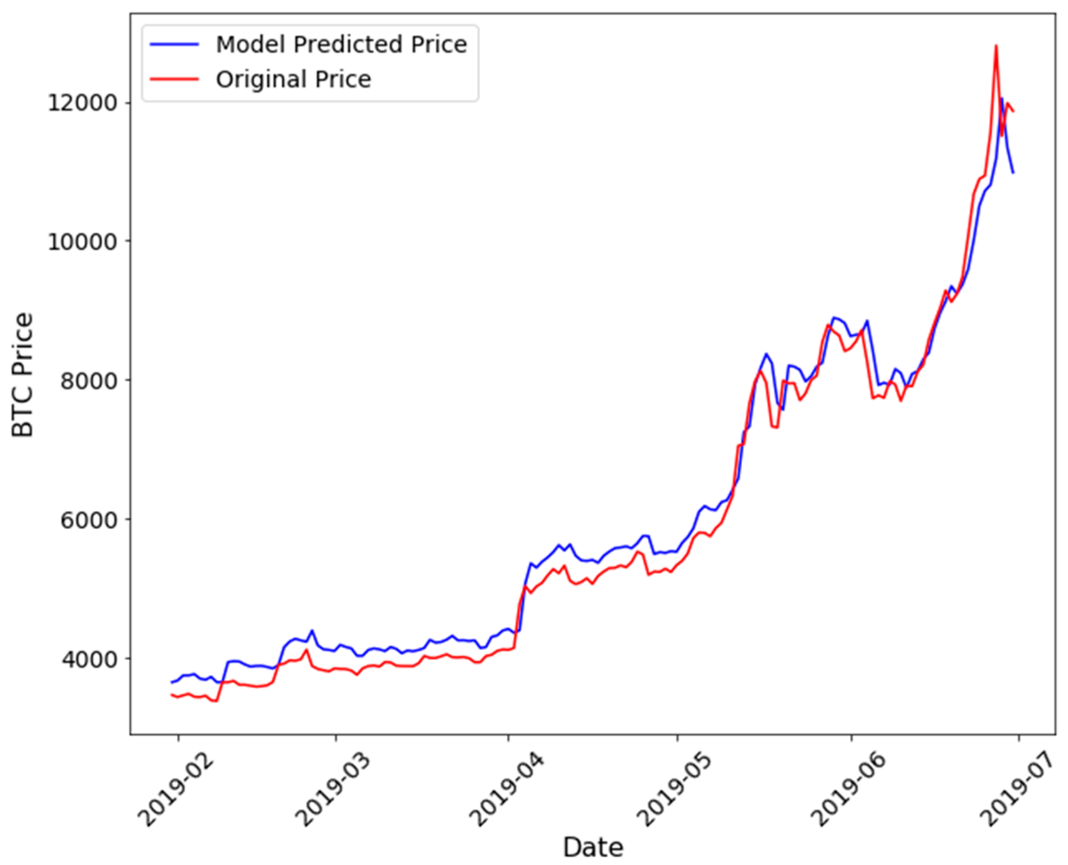
4. Model Implementation and Results

Even though Bitcoin prices follow a time series sequence, machine learning models are considered due to their performance reported in the literature (Karasu et al. 2018; Chen et al. 2020). This approach serves the purpose to measure the relative prediction power of the shallow/deep learning models, as compared to the traditional models. The Bitcoin price graph in Figure 3 appears to be non-stationary with an element of seasonality and trend, and neural network models are the best to capture that. At first, a simple NN architecture was trained to explore the prediction power of non-linear architectures. A set of shallow learning models was then used to predict the Bitcoin prices using various variants of the RNN, as described in Section 2. RNN with a LSTM and GRU with dropout and recurrent dropouts were trained and implemented. Keras package (Chollet 2015) was used with Python 3.6 to build, train, and analyze the models on the test set. A deep learning model implementation approach to forecasting is a trade-off between bias and variance, the two main sources of forecast errors (Yu et al. 2006). Bias error is attributed to inappropriate data assumptions, while variance error is attributed to model data sensitivity (Yu et al. 2006). A low-variance high-bias model leads to underfitting, while a low-bias high-variance model leads to overfitting (Lawrence et al. 1997). Hence, the forecasting approach aimed to find an optimum balance between bias and variance to simultaneously achieve low bias and low variance. In the present study, a high training loss denotes a higher bias, while a higher validation loss represents a higher variance. RMSE is preferred over mean absolute error (MAE) for model error evaluation because RMSE gives relatively high weight to large errors.
Each of the individual models were optimized with hyperparameter tuning for price prediction. The main hyperparameters which require subjective inputs are the learning rate alpha, number of iterations, number of hidden layers, choice of activation function, number of input nodes, drop-out ratio, and batch-size. A set of activation functions were tested, and hyperbolic tangent (TanH) was chosen for optimal learning based on the RMSE error on the test set. TanH suffers from vanishing gradient problem; however, the second derivative can sustain for a long time before converging to zero, unlike the rectified linear unit (ReLU), which improves RNN model prediction. Initially, the temporal length, i.e., the look-back period, was taken to be 30 days for the RNN models. The 30-day period was kept in consonance with the standard trading calendar of a month for investment portfolios. Additionally, the best models were also evaluated with a lookback period for 15, 45, and 60 days. The Learning rate is one of the most important hyperparameters that can effectively be used for bias-variance trade-off. However, not much improvement in training was observed by altering the learning rate, thus the default value in the Keras package (Chollet 2015) wa used. We trained all the models with the Adam optimization method (Kingma and Ba 2015). To reduce complex co-adaptations in the hidden units resulting in overfitting (Srivastava et al. 2014), dropout was introduced in the LSTM and GRU layers. Thus, for each training sample the network was re-adjusted and a new set of neurons were dropped out. For both LSTM and GRU architecture, a recurrent dropout rate (Gal and Ghahramani 2016a) of 0.1 was used. For the two hidden layers GRU, a dropout of 0.1 was additionally used along with the recurrent dropout of 0.1. The dropout and recurrent dropout rates were optimized to ensure that the training data was large enough to not be memorized in spite of the noise, and to avoid overfitting (Srivastava et al. 2014). For the simple NN, two dense layers were used with hidden nodes 25 and 1. The LSTM layer was modelled with one LSTM layer (50 nodes) and one dense layer (1 node). The simple GRU and the GRU with recurrent dropout architecture comprised of one GRU layer (50 nodes) and one dense layer with 1 node. The final GRU architecture was tuned with two GRU layers (50 nodes and 10 nodes) with a dropout and recurrent dropout of 0.1. The optimized batch size for the neural network and the RNN models are determined to be 125 and 100, respectively. A higher batch size led to a higher training and validation loss during the learning process.
Figure 5 shows the training and validation loss for the neural network models. The difference between training loss and validation loss reduces with a dropout and a recurrent dropout for the one GRU layer model (Figure 5, bottom middle). However, with the addition of an extra GRU layer, the difference between the training and validation loss increased. After training, all the neural network models were tested on the test data. The RMSE for all the models on the train and test data are shown in Table 1. As seen from Table 2, the LSTM architecture performed better than the simple NN architecture due to memory retention capabilities (Hochreiter and Schmidhuber 1997). As seen from Table 2 the GRU model with a recurrent dropout generates an RMSE of 0.014 on the training set and 0.017 on the test set. RNN-GRU performs better than LSTM, and a plausible explanation is the fact that GRUs are computationally faster with a lesser number of gates and tensor operations. The GRU controls the flow of information like the LSTM unit; however, the GRU has no memory unit and it exposes the full hidden content without any control (Chung et al. 2014). GRUs also tend to perform better than LSTM on less training data (Kaiser and Sutskever 2016) as in the present case, while LSTMs are more efficient in remembering longer sequences (Yin et al. 2017). We also found that the recurrent dropout in the GRU layer helped reduce the RMSE on the test data, and the difference of RMSE between training and test data was the minimum for the GRU model with recurrent dropout. These results indicate that the GRU with recurrent dropout is the best performing model for our problem. Recurrent dropouts help to mask some of the output from the first GRU layer, which can be thought as a variational inference in RNN (Gal and Ghahramani 2016b; Merity et al. 2017). The Diebold-Mariano statistical test (Diebold and Mariano 1995) was conducted to analyze if the difference in prediction accuracy between a pair of models in decreasing order of RMSE is statistically significant. The p-values, as reported in Table 2 and Table 3, indicate that each of the models reported in decreasing order of RMSE, has a significantly improved RMSE than its previous model in predicting Bitcoin prices. We also trained the GRU recurrent dropout model with a lookback period of 15, 45, and 60 days and the results are reported in Table 3. It can be concluded from Table 3 that the lookback period for 30 days is the optimal period for the best RMSE results. Figure 6 shows the GRU model with recurrent dropout predicted Bitcoin price in the test data, as compared to the original data. The model predicted price is higher than the original price in the first few months of 2019; however, when the Bitcoin price shot up in June–July 2019, the model was able to learn this trend effectively.

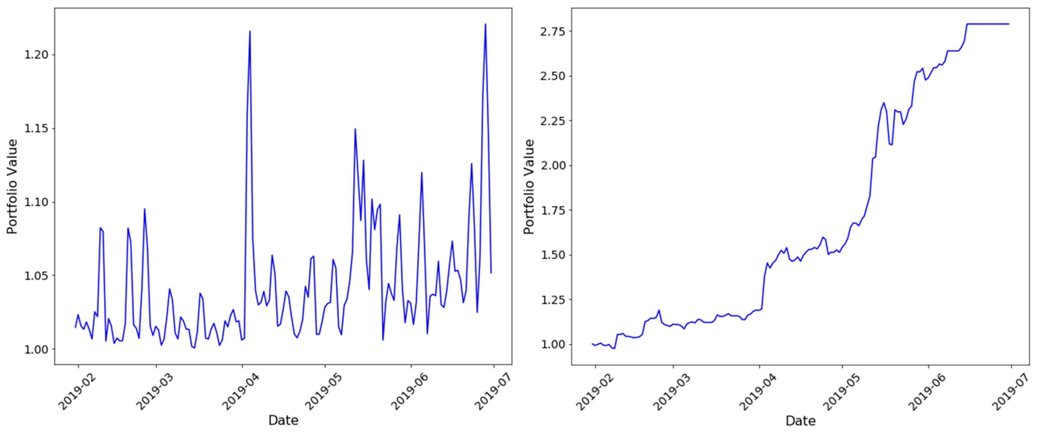
5. Portfolio Strategy

We implement two trading strategies to evaluate our results in portfolio management of cryptocurrencies. For simplicity, we considered only Bitcoin trading and we assumed that the trader only buys and sells based on the signals derived from quantitative models. Based on our test set evaluation, we have considered the GRU one layer with recurrent dropout as our best model for implementing trading strategies. Two types of trading strategies were implemented, as discussed in this section. The first strategy was a long-short strategy, wherein the buy signal predicted from the model will lead to buying the Bitcoin and a sell signal will essentially lead to short-selling the Bitcoin at the beginning of the day based on the model predictions for that day. If the model predicted price on a given day is lower than the previous day, then the trader will short sell the Bitcoin and cover them at the end of the day. An initial portfolio value of 1 is considered and the transaction fees is taken to be 0.8% of the invested or sold amount. Due to daily settlement, the long-short strategy is expected to incur significant transaction costs which may reduce the portfolio value. The second strategy was a buy-sell strategy where the trader goes long when a buy signal is triggered and sell all the Bitcoins when a sell signal is generated. Once the trader sells all the coins in the portfolio, he/she waits for the next positive signal to invest again. When a buy signal occurs, the trader invests in Bitcoin and remains invested till the next sell signal is generated.
Most Bitcoin exchanges, unlike stock exchanges, do now allow short selling of Bitcoin, yet this results in higher volatility and regulatory risks (Filippi 2014). Additionally, volatility depends on how close the model predictions are to the actual market price of Bitcoin at every point of time. As can be seen from Figure 7, Bitcoin prices went down during early June 2019, and the buy-sell strategy correctly predicted the fall, with the trader selling the Bitcoins holding to keep the cash before investing again when the price starts rising from mid-June. In comparison, due to short selling and taking long positions simultaneously, the long-short strategy suffered during the same period of time with very slow increase in portfolio value. However, long-short strategies might be more powerful when we consider a portfolio consisting of multiple cryptocurrencies where investors can take simultaneous long and short positions in currencies, which have significant growth potential and overvalued currencies.

6. Conclusions

There have been a considerable number of studies on Bitcoin price prediction using machine learning and time-series analysis (Wang et al. 2015; Guo et al. 2018; Karakoyun and Çibikdiken 2018; Jang and Lee 2017; McNally et al. 2018). However, most of these studies have been mostly based on predicting the Bitcoin prices based on pre-decided models with a limited number of features like price volatility, order book, technical indicators, price of gold, and the VIX. The present study explores Bitcoin price prediction based on a collective and exhaustive list of features with financial linkages, as shown in Appendix A. The basis of any investment has always been wealth creation either through fundamental investment, or technical speculation, and cryptocurrencies are no exception to this. In this study, feature engineering is performed taking into account whether Bitcoin could be used as an alternative investment that offers investors diversification benefits and a different investment avenue when the traditional means of investment are not doing well. This study considers a holistic approach to select the predictor variables that might be helpful in learning future Bitcoin price trends. The U.S. treasury two-year and ten-year yields are the benchmark indicators for short-term and long-term investment in bond markets, hence a change in these benchmarks could very well propel investors towards alternative investment avenues such as the Bitcoin. Similar methodology can be undertaken for gold, S&P returns and dollar index. Whether it is good news or bad news, increasing attraction or momentum-based speculation, google trends, and VIX price data are perfect for studying this aspect of the influence on the prices.
We also conclude that recurrent neural network models such as LSTM and GRU outperform traditional machine learning models. With limited data, neural networks like LSTM and GRU can regulate past information to learn effectively from non-linear patterns. Deep models require accurate training and hyperparameter tuning to yield results, which might be computationally extensive for large datasets unlike conventional time-series approaches. However, for stock price prediction or cryptocurrency price prediction, market data are always limited and computational complexity is not a concern, and thus shallow learning models can be effectively used in practice. These benefits will likely contribute significantly to quantitative finance in the coming years.
In deep learning literature, LSTM has been traditionally used to analyze time-series. GRU architecture on the other hand, seems to be performing better than the LSTM model in our analysis. The simplicity of the GRU model, where the forgetting and updating is occurring simultaneously, was found to be working well in Bitcoin price prediction. Adding a recurrent dropout improves the performance of the GRU architecture; however, further studies need to be undertaken to explore the dropout phenomenon in GRU architectures. Two types of investment strategies have been implemented with our trained GRU architecture. Results show that when machine learning models are implemented with full understanding, it can be beneficial to the investment industry for financial gains and portfolio management. In the present case, recurrent machine learning models performed much better than traditional ones in price prediction; thus, making the investment strategies valuable. With proper back testing of each of these models, they can contribute to manage portfolio risk and reduce financial losses. Nonetheless, a significant improvement over the current study can be achieved if a bigger data set is available. Convolutional neural network (CNN) has also been used to predict financial returns in forecasting daily oil futures prices (Luo et al. 2019). To that end, a potential future research study can explore the performance of CNN architectures to predict Bitcoin prices.

Author Contributions

Conceptualization, data curation, validation, and draft writing, S.K.; methodology, formal analysis, draft preparation, and editing, A.D.; draft writing, plots, M.B. All authors have read and agreed to the published version of the manuscript.

Funding

This research received no external funding.

Acknowledgments

The authors would like to thank the staff at the Haas School of Business, University of California Berkeley and Katz Graduate School of Business, University of Pittsburgh for their support. A.D.

Conflicts of Interest

The authors declare no conflicts of interest. The views expressed are personal.

Appendix A

Table A1. Definition of variables and data source.
FeaturesDefinitionSource
Bitcoin PriceBitcoin prices.https://charts.bitcoin.com/btc/
BTC Price VolatilityThe annualized daily volatility of price changes. Price volatility is computed as the standard deviation of daily returns, scaled by the square root of 365 to annualize, and expressed as a decimal.https://charts.bitcoin.com/btc/
BTC Miner RevenueTotal value of Coinbase block rewards and transaction fees paid to miners. Historical data showing (number of bitcoins mined per day + transaction fees) * market price.https://www.quandl.com/data/BCHAIN/MIREV-Bitcoin-Miners-Revenue
BTC Transaction VolumeThe number of transactions included in the blockchain each day.https://charts.bitcoin.com/btc/
Transaction FeesTotal amount of Bitcoin Core (BTC) fees earned by all miners in 24-hour period, measured in Bitcoin Core (BTC).https://charts.bitcoin.com/btc/
Hash RateThe number of block solutions computed per second by all miners on the network.https://charts.bitcoin.com/btc/
Money SupplyThe amount of Bitcoin Core (BTC) in circulation.https://charts.bitcoin.com/btc/
Metcalfe-UTXOMetcalfe’s Law states that the value of a network is proportional to the square of the number of participants in the network.https://charts.bitcoin.com/btc/
Block SizeMiners collect Bitcoin Core (BTC) transactions into distinct packets of data called blocks. Each block is cryptographically linked to the preceding block, forming a "blockchain." As more people use the Bitcoin Core (BTC) network for Bitcoin Core (BTC) transactions, the block size increases.https://charts.bitcoin.com/btc/
Google TrendsThis is the month-wise Google search results for the Bitcoins.https://trends.google.com
Volatility (VIX)VIX is a real-time market index that represents the market’s expectation of 30-day forward-looking volatility.http://www.cboe.com/products/vix-index-volatility/vix-options-and-futures/vix-index/vix-historical-data
Gold price LevelGold price level.https://www.quandl.com/data/WGC/GOLD_DAILY_USD-Gold-Prices-Daily-Currency-USD
US Dollar IndexThe U.S. dollar index (USDX) is a measure of the value of the U.S. dollar relative to the value of a basket of currencies of the majority of the U.S.’ most significant trading partners.https://finance.yahoo.com/quote/DX-Y.NYB/history?period1=1262332800&period2=1561878000&interval=1d&filter=history&frequency=1d
US Bond Yields2-year / short-term yields.https://www.quandl.com/data/USTREASURY/YIELD-Treasury-Yield-Curve-Rates
US Bond Yields10-year/ long term yields.https://www.quandl.com/data/USTREASURY/YIELD-Treasury-Yield-Curve-Rates
US Bond YieldsDifference between 2 year and 10 year/ synonymous with yield inversion and recession predictionhttps://www.quandl.com/data/USTREASURY/YIELD-Treasury-Yield-Curve-Rates
MACDMACD=12-Period EMA −26-Period EMA. We have taken the data of the MACD with the signal line.
MACD line = 12-day EMA Minus 26-day EMA
Signal line = 9-day EMA of MACD line
MACD Histogram = MACD line Minus Signal line
Ripple PriceThe price of an alternative cryptocurrency.https://coinmarketcap.com/currencies/ripple/historical-data/?start=20130428&end=20190924
One Day Lagged S&P 500 Market ReturnsStock market returns.https://finance.yahoo.com/quote/%5EGSPC/history?period1=1230796800&period2=1568012400&interval=1d&filter=history&frequency=1d
Interest RatesThe federal funds rate decide the shape of the future interest rates in the economy.http://www.fedprimerate.com/fedfundsrate/federal_funds_rate_history.htm#current

References

  1. Baek, Chung, and Matt Elbeck. 2015. Bitcoin as an Investment or Speculative Vehicle? A First Look. Applied Economics Letters 22: 30–34. [Google Scholar] [CrossRef]
  2. Barrdear, John, and Michael Kumhof. 2016. The Macroeconomics of Central Bank Issued Digital Currencies. SSRN Electronic Journal. Available online: https://papers.ssrn.com/sol3/papers.cfm?abstract_id=2811208 (accessed on 2 February 2020).
  3. Baronchelli, Andrea. 2018. The emergence of consensus: A primer. Royal Society Open Science 5: 172189. [Google Scholar] [CrossRef] [Green Version]
  4. Bech, Morten L., and Rodney Garratt. 2017. Central Bank Cryptocurrencies. BIS Quarterly Review 2017: 5–70. [Google Scholar]
  5. Blau, Benjamin M. 2017. Price Dynamics and Speculative Trading in Bitcoin. Research in Internatonal Business and Finance 41: 493–99. [Google Scholar] [CrossRef]
  6. Blundell-Wignall, Adrian. 2014. The Bitcoin Question: Currency versus Trust-less Transfer Technology. OECD Working Papers on Finance, Insurance and Private Pensions 37: 1. [Google Scholar]
  7. Bohme, Rainer, Nicolas Christin, Benjamin Edelman, and Tyler Moore. 2015. Bitcoin: Economics, technology, and governance. Journal of Economic Perspectives (JEP) 29: 213–38. [Google Scholar] [CrossRef] [Green Version]
  8. Bouri, Elie, Peter Molnár, Georges Azzi, and David Roubaud. 2017. On the hedge and safe haven properties of Bitcoin: Is it really more than a diversifier? Finance Research Letters 20: 192–98. [Google Scholar] [CrossRef]
  9. Briere, Marie, Kim Oosterlinck, and Ariane Szafarz. 2015. Virtual currency, tangible return: Portfolio diversification with bitcoin. Journal Asset Management 16: 365–73. [Google Scholar] [CrossRef]
  10. Cagli, Efe C. 2019. Explosive behavior in the prices of Bitcoin and altcoins. Finance Research Letters 29: 398–403. [Google Scholar] [CrossRef]
  11. Casey, Michael J., and Paul Vigna. 2015. Bitcoin and the digital-currency revolution. The Wall Street Journal. Available online: https://www.wsj.com/articles/the-revolutionary-power-of-digital-currency-1422035061 (accessed on 2 February 2020).
  12. Chang, Pei-Chann, Chen-Hao Liu, Chin-Yuan Fan, Jun-Lin Lin, and Chih-Ming Lai. 2009. An Ensemble of Neural Networks for Stock Trading Decision Making. In Emerging Intelligent Computing Technology and Applications. With Aspects of Artificial Intelligence 5755 of Lecture Notes in Computer Science. Berlin/Heidelberg: Springer, pp. 1–10. Available online: https://doi.org/10.1007/978-3-642-04020-7_1 (accessed on 2 February 2020).
  13. Cheah, Eng-Tuck, and John Fry. 2015. Speculative bubbles in Bitcoin markets? An empirical investigation into the fundamental value of Bitcoin. Economics Letters 130: 32–36. [Google Scholar] [CrossRef] [Green Version]
  14. Chen, Zheshi, Chunhong Li, and Wenjun Sun. 2020. Bitcoin price prediction using machine learning: An approach to sample dimension engineering. Journal of Computational and Applied Mathematics 365: 112395. [Google Scholar] [CrossRef]
  15. Cho, Kyunghyun, Bart van Merrienboer, Caglar Gulcehre, Dzmitry Bahdanau, Bougares Fethi, Schwenk Holger, and Yoshua Bengio. 2014. Learning Phrase Representations using RNN Encoder–Decoder for Statistical Machine Translation. Available online: https://arxiv.org/abs/1406.1078.pdf (accessed on 2 February 2020).
  16. Chollet, Francois. 2015. Keras: Deep Learning for humans. Available online: https://github.com/keras-team/keras (accessed on 2 February 2020).
  17. Chong, Eunsuk, Chulwoo Han, and Frank C. Park. 2017. Deep learning networks for stock market analysis and prediction: methodology, data representations, and case studies. Expert System with Applications 83: 187–205. [Google Scholar] [CrossRef] [Green Version]
  18. Chung, Junyoung, Caglar Gulcehre, Kyung H. Cho, and Yoshua Bengio. 2014. Empirical Evaluation of Gated Recurrent Neural Networks on Sequence Modeling. Available online: https://arxiv.org/pdf/1412.3555.pdf (accessed on 2 February 2020).
  19. Ciaian, Pavel, Miroslava Rajcaniova, and d’Artis Kancs. 2016. The economics of Bitcoin price formation. Applied Economics 48: 1799–815. [Google Scholar] [CrossRef] [Green Version]
  20. Corbet, Shaen, Brian Lucey, Maurice Peat, and Samuel Vigne. 2018. Bitcoin Futures—What use are they? Economics Letters 172: 23–27. [Google Scholar] [CrossRef] [Green Version]
  21. Cusumano, Michael A. 2014. The Bitcoin ecosystem. Communications of the ACM 57: 22–24. [Google Scholar] [CrossRef]
  22. Cybenko, George. 1989. Approximation by superpositions of a sigmoidal function. Math. Control Signals Systems 2: 303–14. [Google Scholar] [CrossRef]
  23. Diebold, Francis X., and Mariano Roberto S. 1995. Comparing Predictive Accuracy. Journal of Business and Economic Statistics 13: 253–63. [Google Scholar]
  24. Dow, Sheila. 2019. Monetary Reform, Central Banks and Digital Currencies. International Journal of Political Economy 48: 153–73. [Google Scholar] [CrossRef]
  25. Dyhrberg, Anne H. 2016. Bitcoin, gold and the dollar-A Garch volatility. Finance Research Letters 16: 85–92. [Google Scholar] [CrossRef] [Green Version]
  26. Dwyer, Gerald P. 2015. The economics of Bitcoin and similar private digital currencies. Journal of Financial Stability 17: 81–91. [Google Scholar] [CrossRef] [Green Version]
  27. ElBahrawy, Abeer, Laura Alessandretti, Anne Kandler, Romualdo Pastor-Satorras, and Andrea Baronchelli. 2017. Evolutionary dynamics of the cryptocurrency market. Royal Society Open Science 4: 170623. [Google Scholar] [CrossRef] [PubMed] [Green Version]
  28. Enke, David, and Suraphan Thawornwong. 2005. The use of data mining and neural networks for forecasting stock market returns. Expert Systems with Applications 29: 927–40. [Google Scholar] [CrossRef]
  29. Fama, Marco, Andrea Fumagalli, and Stefano Lucarelli. 2019. Cryptocurrencies, Monetary Policy, and New Forms of Monetary Sovereignty. International Journal of Political Economy 48: 174–94. [Google Scholar] [CrossRef]
  30. Fantacci, Luca. 2019. Cryptocurrencies and the Denationalization of Money. International Journal of Political Economy 48: 105–26. [Google Scholar] [CrossRef]
  31. Filippi, Primavera De. 2014. Bitcoin: A Regulatory Nightmare to a Libertarian Dream. Internet Policy Review 3. [Google Scholar] [CrossRef]
  32. Gajardo, Gabriel, Werner D. Kristjanpoller, and Marcel Minutolo. 2018. Does Bitcoin exhibit the same asymmetric multifractal cross-correlations with crude oil, gold and DJIA as the Euro, Great British Pound and Yen? Chaos, Solitons & Fractals 109: 195–205. [Google Scholar]
  33. Gal, Yarin, and Zoubin Ghahramani. 2016. Dropout as a Bayesian Approximation: Representing Model Uncertainty in Deep Learning. Available online: https://arxiv.org/pdf/1506.02142.pdf (accessed on 2 February 2020).
  34. Gal, Yarin, and Zoubin Ghahramani. 2016. A theoretically grounded application of dropout in recurrent neural networks. Advances in Neural Information Processing Systems 2016: 1019–27. [Google Scholar]
  35. Gandal, Neil, and Hanna Halaburda. 2016. Can we predict the winner in a market with network effects? Competition in cryptocurrency market. Games 7: 16. [Google Scholar] [CrossRef] [Green Version]
  36. Guo, Tian, Albert Bifet, and Nino Antulov-Fantulin. 2018. Bitcoin volatility forecasting with a glimpse into buy and sell orders. Paper presented at 2018 IEEE International Conference on Data Mining (ICDM), Singapore, November 17–20. [Google Scholar]
  37. Guo, Tian, and Nino Antulov-Fantulin. 2018. Predicting Short-Term Bitcoin Price Fluctuations from Buy and Sell Orders. Available online: https://arxiv.org/pdf/1802.04065v1.pdf (accessed on 2 February 2020).
  38. Hair, Joseph F., Rolph E. Anderson, and Ronald L. Tatham. 1992. Multivariate Data Analysis, 3rd ed. New York: Macmillan. [Google Scholar]
  39. Hileman, G, and M. Rauchs. 2017. Global Cryptocurrency Bench- marking Study. Cambridge Centre for Alternative Finance. Available online: https://www.jbs.cam.ac.uk/fileadmin/user_upload/research/centres/alternative-finance/downloads/2017-04-20-global-cryptocurrency-benchmarking-study.pdf (accessed on 2 February 2020).
  40. Hinton, Geoffrey E., Simon Osindero, and Yee-Whye The. 2006. A fast learning algorithm for deep belief nets. Neural Computation 18: 1527–54. [Google Scholar] [CrossRef]
  41. Hochreiter, Sepp, and Jürgen Schmidhuber. 1997. Long Short-Term Memory. Neural Computation 9: 1735–80. [Google Scholar] [CrossRef]
  42. Hochreiter, Sepp. 1998. The Vanishing Gradient Problem During Learning Recurrent Neural Nets and Problem Solutions. International Journal of Uncertainty, Fuzziness and Knowledge-Based Systems 6: 107–16. [Google Scholar] [CrossRef] [Green Version]
  43. Huang, Wei, Yoshiteru Nakamori, and Shou-Yang Wang. 2005. Forecasting stock market movement direction with support vector machine. Computers & Operations Research 32: 2513–22. [Google Scholar]
  44. Huck, Nicolas. 2010. Pairs trading and outranking: The multi-step-ahead forecasting case. European Journal of Operational Research 207: 1702–16. [Google Scholar] [CrossRef]
  45. Jang, Huisu, and Jaewook Lee. 2017. An Empirical Study on Modeling and Prediction of Bitcoin Prices with Bayesian Neural Networks Based on Blockchain Information. IEEE Access 6: 5427–37. [Google Scholar] [CrossRef]
  46. Kaiser, Lukasz, and Ilya Sutskever. 2016. Neural GPUS Learn Algorithms. Available online: https://arxiv.org/pdf/1511.08228.pdf (accessed on 2 February 2020).
  47. Kaiser, Lars. 2019. Seasonality in cryptocurrencies. Finance Research Letters 31: 232–38. [Google Scholar] [CrossRef]
  48. Karakoyun, Ebru Şeyma, and Ali Osman Çıbıkdiken. 2018. Comparison of ARIMA Time Series Model and LSTM Deep Learning Algorithm for Bitcoin Price Forecasting. Paper presented at the 13th Multidisciplinary Academic Conference in Prague 2018 (The 13th MAC 2018), Prague, Czech Republic, May 25–27. [Google Scholar]
  49. Karasu, Seçkin, Aytaç Altan, Zehra Saraç, and Rifat Hacioğlu. 2018. Prediction of Bitcoin prices with machine learning methods using time series data. Paper presented at 26th Signal Processing and Communications Applications Conference (SIU), Izmir, Turkey, May 2–5. [Google Scholar]
  50. Katsiampa, Paraskevi. 2017. Volatility estimation for Bitcoin: A comparison of GARCH models. Economics Letters 158: 3–6. [Google Scholar] [CrossRef] [Green Version]
  51. Kennedy, Peter E. 1992. A Guide to Econometrics. Oxford: Blackwell. [Google Scholar]
  52. Kim, Young B., Jun G. Kim, Wook Kim, Jae H. Im, Tae H. Kim, Shin J. Kang, and Chang H. Kim. 2016. Predicting Fluctuations in Cryptocurrency Transactions Based on User Comments and Replies. PLoS ONE 11: e0161197. [Google Scholar] [CrossRef] [Green Version]
  53. Kingma, Diederik P., and Jimmy Ba. 2015. Adam: A method for stochastic optimization. arXiv 2015: 9. [Google Scholar]
  54. Krafft, Peter M., Nicolas D. Penna, and Alex S. Pentland. 2018. An Experimental Study of Cryptocurrency Market Dynamics. Paper presented at CHI Conference, Montreal, QC, Canada, April 21–26. [Google Scholar]
  55. Kristoufek, Ladoslav. 2015. What Are the Main Drivers of the Bitcoin Price? Evidence from Wavelet Coherence Analysis. PLoS ONE 10: e0123923. [Google Scholar] [CrossRef]
  56. Lawrence, Steve, Giles C. Lee, and Ah C. Tsoi. 1997. Lessons in Neural Network Training: Overfitting May be Harder than Expected. In Proceedings of the Fourteenth National Conference on Artificial Intelligence. Menlo Park: AAAI Press, pp. 540–45. [Google Scholar]
  57. Lo, Stephanie, and J. Christina Wang. 2014. Bitcoin as Money? Working Paper 14. Boston, MA, USA: Federal Reserve Bank of Boston. [Google Scholar]
  58. Luo, Zhaojie, Xiaojing Cai, Katsuyuki Tanaka, Tetsuya Takiguchi, Takuji Kinkyo, and Shigeyuki Hamori. 2019. Can we forecast daily oil futures prices? Experimental evidence from convolutional neural networks. Journal of Risk and Financial Management 12: 9. [Google Scholar] [CrossRef] [Green Version]
  59. Madan, Issax, Saluja Shaurya, and Zhao Aojja. 2015. Automated Bitcoin Trading via Machine Learning Algorithms. Available online: https://pdfs.semanticscholar.org/e065/3631b4a476abf5276a264f6bbff40b132061.pdf (accessed on 2 February 2020).
  60. Malherbe, Leo, Matthieu Montalban, Nicolas Bedu, and Caroline Granier. 2019. Cryptocurrencies and Blockchain: Opportunities and Limits of a New Monetary Regime. International Journal of Political Economy 48: 127–52. [Google Scholar] [CrossRef]
  61. Marquardt, Donald W. 1970. Generalized inverses, ridge regression, biased linear estimation, and nonlinear estimation. Technometrics 12: 591–612. [Google Scholar] [CrossRef]
  62. McNally, Sean, Jason Roche, and Simon Caton. 2018. Predicting the Price of Bitcoin Using Machine Learning. Paper presented at 26th Euromicro International Conference on Parallel, Distributed and Network-based Processing (PDP), Cambridge, UK, March 21–23. [Google Scholar]
  63. Merity, Stephen, Nitish S. Keskar, and Richard Socher. 2017. Regularizing and Optimizing LSTM Language Models. Available online: https://arxiv.org/abs/1708.02182 (accessed on 2 February 2020).
  64. Muzammal, Muhammad, Qiang Qu, and Bulat Nasrulin. 2019. Renovating blockchain with distributed databases: An open source system. Future Generation Computer Systems 90: 105–17. [Google Scholar] [CrossRef]
  65. Nakamoto, Satoshi. 2008. Bitcoin: A Peer-to-Peer Electronic Cash System. Available online: https://bitcoin.org/bitcoin.pdf (accessed on 2 February 2020).
  66. Nawata, Kazumitsu, and Nobuko Nagase. Estimation of sample selection bias models. Econometric Reviews 15: 4. [CrossRef]
  67. Neter, John, William Wasserman, and Michael H. Kutner. 1989. Applied Linear Regression Models. Homewood: Irwin. [Google Scholar]
  68. Pichl, Lukas, and Taisei Kaizoji. 2017. Volatility Analysis of Bitcoin Price Time Series. Quantitative Finance and Economics 1: 474–85. [Google Scholar] [CrossRef]
  69. Poyser, Obryan. 2017. Exploring the Determinants of Bitcoin’s Price: An Application of Bayesian Structural Time Series. Available online: https://arxiv.org/abs/1706.01437 (accessed on 2 February 2020).
  70. Pascanu, Razvan, Tomas Mikolov, and Yochus Bengio. 2013. On the Difficulty of Training Recurrent Neural Networks. Available online: https://arxiv.org/pdf/1211.5063.pdf (accessed on 2 February 2020).
  71. Rogojanu, Angel, and Liana Badeaetal. 2014. The issue of competing currencies. Case study bitcoin. Theoretical and Applied Economics 21: 103–14. [Google Scholar]
  72. Selmi, Refk, Walid Mensi, Shawkat Hammoudeh, and Jamal Boioiyour. 2018. Is Bitcoin a hedge, a safe haven or a diversifier for oil price movements? A comparison with gold. Energy Economics 74: 787–801. [Google Scholar] [CrossRef]
  73. Sheta, Alaa F., Sara Elsir M. Ahmed, and Hossam Faris. 2015. A comparison between regression, artificial neural networks and support vector machines for predicting stock market index. Soft Computing 7: 8. [Google Scholar]
  74. Siami-Namini, Sima, and Akbar S. Namin. 2018. Forecasting Economics and Financial Time Series: ARIMA vs. LSTM. Available online: https://arxiv.org/abs/1803.06386v1 (accessed on 2 February 2020).
  75. Sovbetov, Yhlas. 2018. Factors influencing cryptocurrency prices: Evidence from bitcoin, ethereum, dash, litcoin, and monero. Available online: https://mpra.ub.uni-muenchen.de/85036/1/MPRA_paper_85036.pdf (accessed on 2 February 2020).
  76. Srivastava, Nitish, Geoffrey Hinton, Alex Krizhesvsky, Ilya Sutskever, and Ruslan Salakhutdinov. 2014. Dropout: A Simple Way to Prevent Neural Networks from Overfitting. Journal of Machine Learning Research 15: 1929–58. [Google Scholar]
  77. Wang, Lin, Yi Zeng, and Tao Chen. 2015. Back propagation neural network with adaptive differential evolution algorithm for time series forecasting. Expert Systems with Applications 42: 855–63. [Google Scholar] [CrossRef]
  78. White, Lawrence H. 2015. The market for cryptocurrencies. The Cato Journal 35: 383–402. [Google Scholar] [CrossRef] [Green Version]
  79. Yin, Wenpeng, Katharina Kann, Mo Yu, and Hinrich Schutze. 2017. Comparative Study of CNN and RNN for Natural Language Processing. Available online: https://arxiv.org/pdf/1702.01923.pdf (accessed on 2 February 2020).
  80. Yelowitz, Aaron, and Matthew Wilson. 2015. Characteristics of Bitcoin users: an analysis of Google search data. Applied Economics Letters 22: 1030–36. [Google Scholar] [CrossRef] [Green Version]
  81. Yu, Lean, Kin K. Lai, Shouyang Wang, and Wei Huang. 2006. A Bias-Variance-Complexity Trade-Off Framework for Complex System Modeling. In Computational Science and Its Applications-ICCSA 2006. Lecture Notes in Computer Science. Berlin/Heidelberg: Springer, Volume 3980. [Google Scholar]
Figure 1. Architecture of a long short-term memory (LSTM) cell. +: “plus” operation; : “Hadamard product” operation; σ : “sigmoid” function; tanh: “tanh” function.
Jrfm 13 00023 g001
Figure 2. Architecture of a gated recurring unit (GRU) unit. +: “plus” operation; : “Hadamard product” operation; σ : “sigmoid” function; tanh: “tanh” function.
Jrfm 13 00023 g002
Figure 3. Time series plot of Bitcoin price in USD.
Jrfm 13 00023 g003
Figure 4. Plot showing the behavior of independent variables with Bitcoin price. The blue line plots the different features used for Bitcoin price prediction and the orange line plots the Bitcoin price over time. Abbreviations: MACD, Moving average convergence divergence.
Jrfm 13 00023 g004
Figure 5. Training and validation loss for simple neural network (NN) (top left), LSTM with dropout (top right), GRU (bottom left), GRU with a recurrent dropout (bottom middle), and GRU with dropout and recurrent dropout (bottom right).
Jrfm 13 00023 g005
Figure 6. Bitcoin price as predicted by the GRU one-layer model with dropout and recurrent dropout.
Jrfm 13 00023 g006
Figure 7. Above shows the change in portfolio value over time when the strategies long-short (Left) and buy-sell (Right) are implemented on the test data. Due to short selling, daily settlement the long-short portfolio incurs transaction fees which reduces growth and increases volatility in the portfolio.
Jrfm 13 00023 g007
Table 1. Variance inflation factor (VIF) for predictor variables.
Predictor VariablesVIFPredictor VariablesVIF
Bitcoin daily lag returns1.023Block size30.208
Daily transaction volume2.823MACD histogram1.27
Price volatility1.13S&P lag returns1.005
Transaction fees4.671VIX1.671
Miner revenue28.664Dollar index6.327
Hash rate2.694Gold5.267
Interest rates49.7182 Yr yield3.074
Google trend9.84710 Yr yield8.101
Money supply8.462Ripple price5.866
Metcalf UTXO12.003Diff 2 yr–10 yr diff11.283
Table 2. Train test root mean squared error (RMSE) of 30 days lookback period for different models.
ModelsRMSE TrainRMSE Testp-Value
Neural Network0.0200.031
LSTM0.0100.0240.0000
GRU0.0100.0190.0000
GRU-Dropout0.0140.0170.0012
GRU-Dropout-GRU0.0120.0340.0000
Table 3. Train test RMSE for GRU recurrent model.
Lookback Period (Days)RMSE TrainRMSE Testp-Value
150.0120.016
450.0110.0190.0010
600.0110.0170.0006

