Abstract
Most studies in Vietnam use the Cobb-Douglas production function and its modifications for economic analysis. Extremely rigid presumptions are a main weak point of this functional form, particularly if the elasticity of factor substitution (ES) is equal to one, which hides the role of the ES for economic growth. The CES (constant elasticity of substitution) production function with more flexible presumptions, concretely its ES, is not unitary, and has been used more and more widely in economic investigations. So, this study is conducted to estimate the average ES through the specification of an aggregate CES function for the Vietnamese nonfinancial enterprises. By performing Bayesian nonlinear mixed-effects regression via Random-walk Metropolis Hastings (MH) algorithm, based on the data set of the listed nonfinancial enterprises of Vietnam, the author found that the CES function estimated for the researched enterprises has an ES lower than one, i.e., capital and labor are complimentary. This finding shows that Vietnamese nonfinancial enterprises can confront a downward trend of output growth.
1. Introduction
Since appearing in 1928, the Cobb-Douglas function has been a highly crucial tool in economic research. This functional form has become very popular due to its ease of use and empirical adaptation to different data sets. Solow (1957) and his followers used the Cobb-Douglas in their growth theories. However, this type of function is criticized because of its rigid premises. One of them is the unit ES, which, according to many empirical results, does not coincide with facts. Moreover, the unit ES masks the role of the ES for economic growth processes. Several theoretical and empirical studies published have explored this limitation. For example, among others, Antrás (2004) stated that the ES is not appropriate for the US economy, and Werf (2007) argued that the Cobb-Douglas function is not suitable for modeling policies for climate change, while Young (2013) revealed that the ES of the aggregate production function and the production function of most U.S. industries could not be equal to one and had estimates less than 0.62. Therefore, the CES function with an ES other than one was announced in 1961 (Arrow et al. 1961). Since then, an increasing amount of studies around the world have used the CES function for economic analysis, while the number of works evaluating elasticities using the Cobb-Douglas function decreased substantially. Specifically, Heubes (1972) theoretically argued that either the time path or the level of the output growth rate depends on the ES value. Among empirical studies, Ferguson (1965), La Grandville (1989), Klump and La Grandville (2000), Pitchford (1960), Azariadis (1993), and Galor (1995) focussed on the effects of the ES on economic growth. In Vietnam, to the knowledge of the author, the Cobb-Douglas function and its different modifications are commonly used, and at present, no empirical research on the CES function has been carried out. Besides, most previous research on production functions applied mainly traditional quantitative methods, such as the accounting method or the frequentist approach, being a subject of much criticism from modern statisticians as it gave unreliable results in many cases (Briggs and Nguyen 2019; Anh et al. 2018; Kreinovich et al. 2019).
Because of the above reasons, the author conducted this study to estimate the ES via specifying an aggregate CES function using a non-frequentist method, namely the Bayesian nonlinear mixed-effects regression.
The remainder of the paper is structured as follows. Section 2 introduces the theoretical framework of the ES and its relationship with economic growth. Section 3 provides the theoretical analysis of the ES in the CES. Empirical studies on the ES in the CES and its association with economic growth are reviewed in Section 4. Section 5 discusses the data and estimation method. Bayesian simulation results are provided in Section 6. Section 7 includes the conclusion.
2. Theoretical Background of the ES
2.1. The ES
Production functions are an important instrument of economic analysis in the neoclassical tradition. They are often utilized to analyze the economic performance of an economy, as well as those of enterprises, industries and industrial complexes. Homogeneity and returns to scale particularize a neoclassical production function under the conditions of uniform changes in all inputs. Nonetheless, when the inputs change at different rates, how does the function change? In this case, the nature of the production function varies depending on the ES. In general, the ES plays a significant role in economic growth process.
The marginal rate of technical substitution between two inputs () illustrates the rate at which one input must decrease to hold a production level unchanged when another input increases:
where are the first and second inputs, respectively.
The limitation of this coefficient is that it is dependent on the measurement unit of resources. Therefore, the usage of the ES instead is more appropriate:
where —the ES of input for input
The ES denotes how the ratio of inputs changes if the marginal rate of technical substitution between them varies by one percent. Hicks (1932) first proposed this definition for the case of two inputs. In the case of n inputs, the method of calculating the ES is inconsistent. In a later work of Hicks and Allen (1934), a generalized ES was suggested. Accordingly, the formula for the two-input case is applied to any two inputs in a multivariate function with the assumption that other inputs remain unchanged. This is the Hicks Elasticity of Substitution (HES). However, the restriction of the HES is that because the optimal quantity of all inputs is simultaneously decided by enterprises, the ratio between any two inputs is affected not only by relative prices but also by the prices of other inputs. The optimization behavior of enterprises requires:
then
where are the price of , respectively.
Under the optimization condition, the ES indicates how the input ratio varies if their price ratio changes by one percent. Let us consider a function with three inputs f(. With this preposition, . The HES between and shows how the ratio between them changes if changes by one percent with the assumption of a fixed amount of . However, it is noted that a change of may make the amount of vary due to variations in the ratios of and . Thus, the assumption of a fixed quantity of the third input is not always correct. The use of the HES is correct only for the Cobb-Douglas and the CES because the change in the third input does not impact on the ratio between the first two inputs. In the meanwhile, for generalized functions, the HES may yield biased results.
Hicks and Allen proposed a Partial Elasticity of Substitution to measure the ES. Later, this coefficient was studied in detail by Allen and Uzawa, so it was called the Allen-Uzawa Elasticity of Substitution (AUES). AUES is calculated by the following formula:
where
where denotes algebraic addition to element in .
In the two-input case, AUES is reduced to the HES. Nevertheless, Blackorby and Russell (1981) claim that deduction from the ES between two inputs to the ES between multiple inputs is not correct. They proved the non-informativeness of AUES in several cases. So, the Morishima Elasticity of Substitution (MES) was proposed instead:
where is a cost optimization function derived from:
McFadden (1963) created a new development in the elasticity theory showing the possibility of the ES to have different values for various input pairs. According to this author, it is not possible to construct a neoclassical production function with an arbitrary set of the ES when the number of inputs is more than two. That is, if we propose different ES for various input groups, it is necessary to use a different type of production function that may not be fixed at different input quantities and at various prices.
In this study, the author uses the ES between the two inputs, capital and labor. In this case, the ES is a measure of the ease of substitution between capital and labor, or a measure of their similarity from a technological view. When the ES is large, the inputs are similar to each other. So when an input increases, the technology enables this factor to be easily substituted for the element remaining constant. In the case of a small ES, the technology views the inputs as unsimilar, so it is difficult to substitute one input for the other. In other words, as expressed by Nelson (1965), the ES can be referred to as an index of the rate at which diminishing marginal return sets in as one input increases in relation to the other. If the ES is great, then it is easy to substitute one input for the other or to increase output by increasing one input. Hence, a diminishing marginal return will set in slowly or not set at all. From here, we could confirm that the ES has an effect on the economic growth as long as inputs grow at different rates so their proportions change.
2.2. Impact of the ES on Economic Growth
In order to show the positive effect of the ES on economic growth, let us use a 2-factor linear homogenous production function with Hicks-neutral technical change (A):
Differentiating (1), we get:
As known, Hence, the output growth rate is the following:
We have:
The elasticity of production with respect to labor is written as a function of the ES:
or in logs and differentiating with respect to time:
It is known:
Therefore
and
So, we get:
Assuming the constant growth rates of technical progress and the inputs, the output growth rate () may vary only because of changes in Combining (4) with (10), we obtain:
In case , the sign of (11) will be positive if and negative if . Thus, the magnitude of the ES effects is dependent of the difference between the growth rates of capital and labor. In case , the variation of over time is small or the impact of the ES on economic growth rate is weak.
In addition, Heubes (1972) stated that not only the time path but also the level of the output growth rate are functions of the ES. Let us differentiate (4) with respect to time and to get for small and
In case and , the higher growth rate of output is correlated to a greater ES. Hence, If the ES is low, a strong impact of the relatively scarce input on output emerges as its elasticity of production is great. With a growing the elasticity of production diminishes for the scarce input, but it increases for the relatively abundant factor. The impact of the ES change on the output growth rate becomes small for high levels of the ES. The growth rate is independent of the ES when
3. ES in the CES Function
Before analyzing the ES in the CES, we consider the Cobb-Douglas function. The work of Cobb and Douglas (1928) is a turning point in the field of production functions. It can be said, although there have been some previous studies on production functions (see Schumpeter 1954; Stigler 1952; Barkai 1959; Lloyd 1969; Velupillai 1973; Samuelson 1979; Humphrey 1997), for the first time the relationship between inputs and outputs is mathematically formulated and empirically assessed in (Cobb and Douglas 1928). During a vacation at Amherst, Paul Douglas asked math professor Charles Cobb to suggest an equation describing the relationship between capital and labor and output based on time series data on the U.S. manufacturing sector for the period 1889–1922. As a result, a joint paper showed up, where the authors concluded that their model fits the data well. The initial Cobb-Douglas function has the following form:
where is capital (), is labor (); are parameters.
However, in the later works, Douglas removed the assumption that sum of elasticities of output by capital and labor equals one, and used the functional form (14):
where A denotes technical change; are exponentials and elasticities of output by capital and labor, respectively.
The Cobb-Douglas has some properties. First, it belongs to the neoclassical class with , and therefore, reflects the law of positive and diminishing marginal productivity. Second, its homogeneity is + In case +, we get a linear homogenous function. If , then the multiplicative function points to a growing economic system as the output grows faster than the inputs. Then, returns to scale increase. Meanwhile, if , returns to scale decrease. denotes constant returns to scale. Returns to scale are also the homogeneity of the production function and equal to
where
As we know, in the Cobb-Douglas function, the ES equals one.
Although the Cobb-Douglas is a powerful mathematical tool to describe production processes, as mentioned above, this functional form has extremely rigid premises. Hence, the CES function came into sight. The CES was established by Arrow et al. (1961) or ACMS for short. The authors dedicated the analysis to the ES. The production functions at that time assumed that the ES receives a fixed value, such as zero for Leontieff and one for Cobb-Douglas, which, in their view, is too rigid. Moreover, in order to assess the impact of economic policies on factor income, the CES is more appropriate (Miller 2008) or the Cobb-Douglas hides the role of the ES on economic growth and technical progress (Pereira 2003).
To examine the goodness of fit of the Leontieff and Cobb-Douglas functions, ACMS performed econometric analysis of the behavior of the ratio of labor income to nominal output. As long as output and input prices remain unchanged, the proportion is fixed and determined only by the parameters of the function. Rejection of the Cobb-Douglas (and Leontieff) functions are based on the arguments below.
The invariance of labor share in the Cobb-Douglas is expressed as follows:
Equation (16) is rewritten in logs:
where
For the Leontieff function, the ratio between inputs arises from the production process, but is not influenced by price, i.e.,:
Equation (18) takes the form of logs:
where
Hence, we need to analyze the following function:
where is a random error.
It is necessary to test the hypotheses Investigating a data sample of 24 industries of 19 countries, ACMS came to the conclusion that, in most cases, the hypotheses are rejected.
The above finding encouraged the researchers to construct a new type of production function with a more flexible labor share, which is expressed in the following:
where parameter can have any value, but not zero or one.
From (21), under a condition of nonexistence of restraints on we can get a CES function. Through some transformations, the last version of the CES is the following:
where = is substitution parameter, is distribution parameter; is efficiency parameter and , the ES,
So that the CES function (22) is a neoclassical one, assumptions must be made. The premise of Hicks-neutral technical progress in the CES implies that the output produced by combining capital with labor is assumed to grow exponentially in a way that does not alter the marginal rate of technical substitution between the inputs. Therefore, the parameters of the production function will be stable over time.
In case , i.e., capital and labor are substitutable, so rising leads to an increase in capital share.
If , i.e., capital and labor are complementary, and thus, when increases, labor share rises.
In case (), then the Cobb-Douglas is obtained.
4. Empirical Research on the Elasticity of Factor Substitution and Its Association with Economic Growth
4.1. Estimation of the ES
Solow (1957) was a pioneer, and his followers used the Cobb-Douglas function, where technical change is referred to as neutral, and therefore changes in the ES were completely ignored (the ES is always equal to one). In their models, technical change is called total factor productivity (TFP). Nevertheless, in many empirical studies, the ES varies. For example, among others, Nerlove (1967) on a survey found that changes in period or concept may generate the different values of the ES. Comparing ES estimates from six alternative functional forms, five different measures of the rental price of capital, and two estimation techniques, Berndt (1976) went to a similar conclusion. McFadden (1978) tested the constancy of the ES for the steam-electric generating industry and revealed that the ES obtains a value of approximately 0.75. Hamermesh (1993) showed that the ES varies from 0.32 to 1.16 in the US and from 0.49 to 6.86 in the UK.
The consideration of the U.S. processing industry over a 200-year period indicates that ES values tend to change. The evidence shows that the ES was close to zero in the 19th century (Asher 1972; Uselding 1972; Schmitz 1981), close to one in the mid-20th century (Zarembka 1970), and greater than one in the late 20th century (Blair and Kraft 1974; Hsing 1996). Duffy and Papageorgiou (2000) estimated the ES based on a CES function on a cross-section of 82 countries and found the ES greater than one for developed economies and lower than one for developing economies. These authors concluded that the ES level is related to a country’s stages of development. Using a Variable Elasticity of Substutution (VES) for 12 OECD countries (1965–1986), Genç and Bairam (1998) revealed that the average ES is greater than one. It is noteworthy that the diversity of results is because of the difference in data sets and estimation techniques. The above analyses also revealed that the ES is stable for a sample period, but rises with economic development.
4.2. Impact of the ES on Economic Growth
Theoretically, in early growth theory, some authors attempted to prove the significance of the ES. Solow (1957), Pitchford (1960), and Sato (1963) stated that allowing the ES to get any value will generate multiple growth paths, and some of them will be unbalanced. Recently, Azariadis (1993), using the overlapping generations model of growth, showed the possibilities of poverty traps depending on the values of the ES.
Ferguson (1965) ensured that in the case of a non-unitary ES, the output growth rate is dependent on the ES, as well as the growth rate of the savings ratio. La Grandville (1989), making use of the Slutsky equation, provided another evidence on the positive relationship between the ES and the output. The larger the ES, the higher production level that can be obtained. Barro and Sala-i-Martin (1995) found that under certain conditions, a large ES generates endogenous, steady-state growth. Later, Klump and La Grandville (2000) proved that a greater ES leads to more probable endogenous growth and higher long-term growth rates. Also, the greater the ES, the higher steady-state income per capita. If the ES is more than one, we can achieve a unique steady-state and possibility of endogenous growth (Barro and Sala-i-Martin 1995). In the meantime, Pitchford (1960), Azariadis (1993), and Galor (1995), among others, considered that an ES lower than one in a CES function indicates multiple steady-states and poverty traps for per capita output. Two studies relying on La Grandville conducted by Yuhn (1991) and Cronin et al. (1997) attempted to test the relationship between the ES and economic growth. Comparing the US with South Korea, Yuhn (1991) found that the ES was higher for South Korea, which helps explain the higher growth rates acquired in this country after the 1960s. Utilizing data set for the 1961–1991 period, Cronin et al. (1997) estimated an ES of 13.01 between telecommunication and capital. Changes in the ES affect growth rate since production is an increasing function of the ES. In the CES case, the ES influences growth in almost every case, except when both inputs are increasing at the same rate (Kamien and Schwartz 1968).
Most studies on production functions in Vietnam made use of the frequentist methods or accounting method to estimate the Cobb-Douglas function. As known, this production function has an ES of one. Tu and Nguyen (2012) used the Cobb-Douglas function to analyze the impact of inputs on coffee productivity in DakLak province. Q.H. Nguyen (2013) applied the accounting method to build a Cobb-Douglas function for Hung Yen province to identify the resources of economic growth of this province. Khuc and Bao (2016) built an extended Cobb-Douglas function to identify factors contributing to the Vietnamese industry growth. Using the accounting method, Le estimated Vietnam’s Cobb-Douglas function based on enterprise data of mining, processing industry, electricity and water production and distribution. The results show that the proportion of labor and fixed assets in the total output of the studied sectors ranges from 0.11 to 0.39 and 0.89 to 0.61, respectively.
For other types of the Cobb-Douglas function, Pham and Ly (2016) constructed a translog Cobb-Douglas function for the manufacturing enterprises of Vietnam, having net revenue as the output and capital, labor, and other costs as the inputs, based on data extracted from the 2010 Vietnam Enterprise Survey by the General Statistics Office. Huynh (2019) used the MLE method on a dataset extracted from the Enterprise Survey of the General Statistics Office for the period 2013-2016 to build a Battese-Coelli production function and analyze the factors affecting technical efficiency of small and medium enterprises in Vietnam.
It is noted that in the production function theory, many studies have tried to «soften» the premises of the Cobb-Douglas and the CES. But so far no other functions could surpass them in terms of popularity. Moreover, because of the very rigid premises of the Cobb-Douglas, the CES is increasingly explored. Hence, in the present work, the CES is selected to estimate the ES based on the data set of the Vietnamese nonfinancial enterprises.
5. Methodology and Data
5.1. Method and Model
There are several methods applied to estimate the ES, but different techniques can be divided into two main groups: Direct and indirect. A direct method allows for estimating the ES through the specification of a production function. The indirect method explores the link between the ES and factor shares to obtain the estimates. We can estimate the ES via the first-order profit maximization condition for labor employment. McFadden (1978) considered that choosing estimation methods depends on data availability, while Mizon (1977) preferred the direct method to the indirect way as the former provides estimates for a large number of functional forms using a common estimation technique and data set. In this study, following Mizon (1977), the author chooses the direct method.
Note that most of the previous studies estimated the ES within the frequentist framework using the CES or the VES. However, in the last three decades, the Bayesian approach has been popularized in social sciences thanks to some of its important strengths (Nguyen et al. 2019; Briggs and Nguyen 2019; Thach et al. 2019; Thach 2019). So, the question of when to use Bayesian analysis and when to use frequentist analysis depends on our specific research problem. For instance, firstly, if we would like to estimate the probability that a parameter belongs to a given interval, the Bayesian framework is appropriate. But if we want to perform a repeated-sampling inference about some parameter, the frequentist approach is needed. Secondly, from what was just mentioned, frequentist confidence intervals do not have straightforward probabilistic interpretation compared to Bayesian credible intervals. A 95% confidence interval can be explained as follows: If the same experiment is repeated many times and confidence intervals are computed for each experiment, then 95% of those intervals will contain the true value of the parameter. The probability that the true value falls in any given confidence interval is either one or zero, and we do not know which. Meanwhile, a 95% Bayesian credible interval provides a straightforward interpretation that the probability that a parameter lies in an interval is 95%. Thirdly, frequentist analysis is performed to approximate the true values of unknown parameters, while Bayesian analysis provides the entire posterior distribution of model parameters.
In the current study, making use of the direct method, the author estimates the ES through specifying an aggregate CES function. To estimate the CES function, the Bayesian nonlinear mixed-effects regression is performed. The Bayesian mixed-effects models with the grouping structure of the data consisting of multiple levels of nested groups contain both fixed effects and random effects. Our two-level mixed-effects model accounts for the variability between enterprises, which are identified by the id variable. According to Nezlek (2008), the results of analyses of multilevel data that do not take into account the multilevel nature of the data may (or perhaps will) be inaccurate. Based on Equation (22), our nonlinear model has the following expression:
where is natural logarithm of output, and are natural logarithm of capital and labor used, respectively, is an intercept, is used to calculate , is a random error. The conditions must be satisfied so Equation (23) is a neoclassical function.
In Bayesian analysis, we use conditional probability:
to derive Bayes’s theorem:
where are random vectors.
Assuming that a data vector is a sample from a probability model with the unknown parameter vector , this model is written using a likelihood function:
where is a probability density function of given .
Relying on given data , we infer some properties of In Bayesian analysis, model parameters is a random vector.
We begin Bayesian analysis by specifying a posterior model. The posterior model combines given data and prior information to present the probability distribution of all parameters. Therefore, the posterior distribution has two components: A likelihood function containing information about the model parameters based on observed data, and prior distribution, including known information about the model parameters. By Bayes’ law, the likelihood function and priors are combined to form the posterior model:
Posterior ∝ Likelihood × Prior
Because both and are random variables, we apply Bayes’s theorem to obtain the posterior distribution of given :
where known as the marginal distribution of which is formulated as follows:
where is a likelihood function of y given θ, π(θ) is a prior distribution for θ, m(y) is also known as the prior predictive distribution.
In cases when the posterior distribution is derived in closed form, we can proceed immediately to the inference step. However, except for some special models, the posterior distribution is scarcely available and needs to be estimated through simulation. Bayesian methods can be used to simulate many models. To simulate Bayes models, MCMC algorithms often require effective sampling and verify convergence of MCMC chains to the stationary distribution.
Experience of fitting Bayesian models shows that the specification of priors can rest on previous studies and expert knowledge. In our research, the propositions of a neoclassical production functions and previous research can suggest us to specify priors. To specify the CES, referring to Arrow et al. (1961), Afees (2015) or Lagomarsino (2017), we proposed to assign the normal N(1,100) prior to parameter , the uniform(0,1) prior to parameter , the gamma(1,1) prior to parameter , and the Igamma(0.001, 0.001) prior to the variance component for () and the overall variance parameter () in this research.
Our Bayesian nonlinear mixed-effects regression model is as follows:
The likelihood function:
The priors:
where are natural logarithm of output, capital, labor employed, respectively in constant 2010 prices, is efficiency parameter, is substitution parameter, is distribution parameter, is the random error, year = 2008,…, 2018, and enterprise = 1, 2, 3,…, 227.
5.2. Data Description
The study utilizes panel data collected from the financial statements and annual reports of 227 non-financial enterprises listed at Ho Chi Minh Stock Exchange and Ha Noi Stock Exchange in Vietnam for the period 2008–2018. All these enterprises belong to different manufacturing industries and thus, to capture their varying effects on the outcome, we perform the mix-effects regression. Time frequency indicates the year. The dataset has 1,974 observations. In Bayesian statistics, due to combining prior information with observed data, inferential results are valid to sparse data, and thus a small sample does not affect MCMC simulation results. It is noted that the 2008–2018 sample period includes years 2008–2009, when many countries around the world faced a sharp economic decline, but the Vietnamese enterprises were much less impacted by this global crisis. Statistical figures show that the economic growth of Vietnam achieved good performance, 5.7%, in 2008, and 5.4% in 2009 (World Bank 2019). Net revenue and fixed assets represent the enterprises’ output and capital variables. The figures of net revenue and fixed assets are calculated based on the 2010 production price index of the General Statistics Office. The units of net revenue, fixed assets and labor are million VND, million VND and number of employees, respectively. The nonfinancial enterprises are chosen for our analysis since this sector is a powerful engine of Vietnamese economic growth, so to a great extent it stands for the national production. Moreover, according to Karabarbounis and Neiman (2014), the use of data on the enterprises listed on the stock market allows labor and capital shares not to be skewed owing to statistical errors that often occur when we take into account the mixed incomes from households’ labor and capital contributions as well as those in the state-owned sector which are difficult to be measured accurately. The measurements of the variables are presented in Table 1.

Table 1.
The measurements of the variables.
6. Empirical Results
6.1. Descriptive Statistics
Table 2 shows that variables y2010, l, and k2010 obtain maximum value of 4.00 × 10⁷, 19,828 and 2.27 × 10⁷, minimum value of 5320, 17 and 270, mean of 1,519,804, 1186 and 497,570, respectively. Standard deviation (Std. Dev) measures the variation or dispersion of a set of values. It equals 3,516,699, 1793 and 1,614,555 for y2010, l and k2010, respectively.
Table 2.
Descriptive statistics.
6.2. Bayesian Simulation Results
Acceptance rate and efficiency are two criteria for evaluating the efficiency of MCMC sampling in Bayesian models. The acceptance rate is the number of proposals accepted in the total number of proposals, while efficiency means the mixing properties of MCMC sampling. Both of these rates influence MCMC convergence. The simulation results demonstrate that our model has a high acceptance rate of 0.6. According to Roberts and Rosenthal (2001), acceptance rates between 0.15–0.5 are optimal. Therefore, the MCMC sampling of our regression model has reached an acceptable acceptance rate. The smallest, average and largest efficiency of the MCMC sampling is 0.044, 0.21 and 0.97, which are greater than the warning level of 0.01 (Table 3). The MC errors (MCSE) of the posterior mean estimates are close to one decimal. The smaller these values are, the more accurate the estimates. In Bayesian analysis, posterior confidence intervals, as stated above, have a straightforward probability interpretation. For example, for our model, the probability of the posterior mean of the parameter in the range (10.7; 11.2) is 95% (Table 3).
Table 3.
Estimation results of the model.
Random intercepts for (id) denote the varying effects of 227 enterprises studied on the outcome of the model. Means of all the random effects get MCSE close to one decimal, which is reasonable for MCMC algorithms. For illustration, we demonstrate the random intercepts of the first 10 enterprises in Table 4.
Table 4.
Estimated random effects of the first 10 enterprises.
6.3. Convergence Test for MCMC Chains
The convergence of MCMC chains should be tested before Bayes inference is performed, because Bayesian inference is robust only when the MCMC chains converge to a stationary distribution. According to the results recorded in Figure 1, with respect to our model, the diagnostic graphs are reasonable. Trace plots exhibiting no trends, run relatively quickly through the distribution towards the constant values of mean and variance; the autocorrelation plots are acceptable; histograms resemble the shape of probability distributions (Figure 1). In general, MCMC chains of our model have good mixing. Therefore, it can be concluded that there is no serious convergence problem and the MCMC chains have converged to the target distribution.
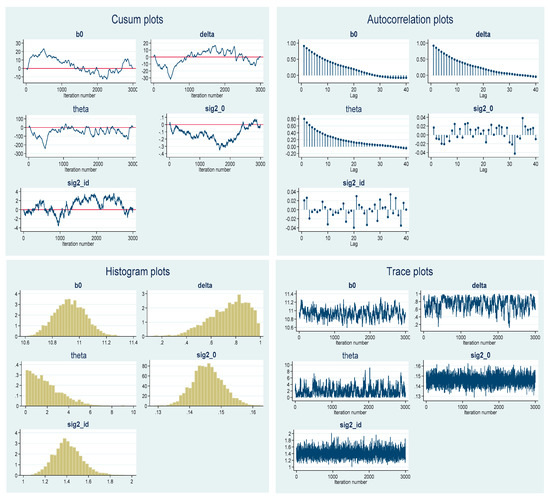
Figure 1.
Graphical convergence diagnostics.
In addition, cusum plots are also a visual method for inspecting MCMC convergence. In our case, the cusum lines are not smooth but jagged, which surely points to MCMC convergence (Figure 1).
Besides visual inspection, formal test in which effective sample size can be used is a common method (Table 5). Efficiency greater than one is suggested satisfactory. Results presented in Table 5 demonstrate no sign of a non-convergence problem since the efficiency of all the model parameters is more than 4, whereas the highest correlation time is 22 lags.
Table 5.
Effective sample size.
6.4. Estimation Result of the ES
According to the results shown in Table 3, our estimated CES function has the value of efficiency parameter = 10.9, a distribution parameter of = 0.7, and a substitution parameter of = 1.9. The Bayesian simulations do not provide point estimates in a frequentist sense. Tests for MCMC convergence allow to confirm whether or not estimation results are robust. In our work, we already performed the convergence diagnostics, which produced acceptable results, as shown in the above. Once Bayesian inference is valid, MCMC iterations do yield similar estimates of the model parameters. These estimates point to the properties of a neoclassical production function. Because the ES is smaller than one . These empirical results coincide with most of previous studies (for example, Berndt 1976; Hamermesh 1993; Pereira 2003; Chirinko 2008; Young 2013). In case , we can provide two main explanations for the Vietnamese nonfinancial enterprises’ output growth.
First, our data set used in this study indicates that there is a marked difference between the growth rates of capital and labor. Hence, with the ES lower than one, the sign of (12) is negative. Based on this finding, it can be concluded that the output growth rate of the Vietnamese nonfinancial enterprises has a falling trend in the long run. We should note that compared to enterprises in advanced economies, the Vietnamese ones have a very low contribution of technical change to production, and hence they are not capable of generating the unbounded endogenous growth. Therefore, stimulating R&D activities in enterprises is extremely important.
Second, as and , the higher growth rate of output is associated with a larger ES, i.e., According to our result, the ES is less than one, so capital as a relatively scarce factor strongly influences the output since its elasticity of production is great (. While the ES is rising, the elasticity of production will be diminishing for the capital, but it will increase for the labor. Under the current conditions of the Vietnamese economy, capital is a scarce factor of the economy, so substantially increasing investment should be one of the most significant growth policies. Specifically, it is necessary to attract more foreign direct investment and expand positive spillover effects from foreign corporations to the national enterprises.
7. Conclusions
The present research uses the Bayesian non-linear mixed-effects regression method via the Random-walk MH algorithm to estimate the ES of the CES production function for nonfinancial businesses listed at Hanoi Stock Exchange and Ho Chi Minh City Stock Exchange in Vietnam. The CES was chosen over the Cobb-Douglas because its premises are more flexible, and in particular, its ES shall have useful implications for economic growth. The results of the convergence tests show that the MCMC chains converge to the target distribution so that the Bayesian inference is robust. Besides, the results of the statistical tests point out that our estimated model is consistent with the observed data. Mixed-effects estimates denote the varying impact of the studied enterprises on the model outcome. The CES function specified is a neoclassical one with a constant ES of less than one, i.e., capital and labor are complementary. So, it is concluded that the output growth rate of the Vietnamese nonfinancial enterprises is going down in the long-term. Thus, Vietnamese enterprises need to expand investment and intensify R&D activities in order to increase the capital-labor ratio as well as the contribution of technical progress to production, thanks to which the possibility of the unceasing endogenous growth can be created in the earliest prospect.
Funding
This research is supported by the Banking University HCMC, Vietnam.
Acknowledgments
The author is thankful to the anonymous referees for very useful comments.
Conflicts of Interest
The author declares no conflict of interest.
References
- Afees, Salisu. 2015. Nonlinear Regression. Center for Econometric and Allied Research. Available online: http://cear.org.ng/index.php?option=com_docman&task=doc_details&gid=33&Itemid=92 (accessed on 10 January 2020).
- Anh, Ly H., Si D. Le, Vladik Kreinovich, and Nguyen Ngoc Thach, eds. 2018. Econometrics for Financial Applications. Cham: Springer. [Google Scholar]
- Antrás, Pol. 2004. Is the US Aggregate Production Function Cobb-Douglas? New Estimates of the Elasticity of Substitution. Contributions to Macroeconomics 4: 1–34. [Google Scholar] [CrossRef]
- Arrow, Kenneth J., Hollis B. Chenery, Bagicha Singh Minhas, and Robert M. Solow. 1961. Capital Labour Substitution and Economic Efficiency. Review of Econ. and Statistics 63: 225–50. [Google Scholar] [CrossRef]
- Asher, Ephraim. 1972. Industrial efficiency and biased technological change in American and British manufacturing: The case of textiles in the nineteenth century. Journal of Economic History 32: 431–42. [Google Scholar] [CrossRef]
- Azariadis, Costas. 1993. Intertemporal Macroeconomics. Hoboken: Blackwell Publishers. [Google Scholar]
- Barkai, Haim. 1959. Ricardo on Factor Prices and Income Distribution in a Growing Economy. Economica 26: 240–50. [Google Scholar] [CrossRef]
- Barro, Robert J., and Xavier Sala-i-Martin. 1995. Economic Growth. New York: McGraw-Hill. [Google Scholar]
- Berndt, Ernst. 1976. Reconciling Alternative Estimates of the Elasticity of Substitution. Review of Economics and Statistics 58: 59–68. [Google Scholar] [CrossRef]
- Blackorby, Charles, and R. Robert Russell. 1981. The Morishima Elasticity of Substitution; Symmetry, Constancy, Separability, and its Relationship to the Hicks and Allen Elasticities. Review of Economic Studies 48: 147–58. [Google Scholar] [CrossRef]
- Blair, Roger, and John Kraft. 1974. Estimation of elasticity of substitution in American manufacturing industry from pooled cross-section and time series observations. Review of Economics and Statistics 56: 343–47. [Google Scholar] [CrossRef]
- Briggs, William, and Hung T. Nguyen. 2019. Clarifying ASA’s View on P-Values in Hypothesis Testing. Asian Journal of Economics and Banking 3: 1–16. [Google Scholar]
- Chirinko, Robert. 2008. The Long and Short of It. Journal of Macroeconomics 30: 671–86. [Google Scholar] [CrossRef]
- Cobb, Charles W., and Paul H Douglas. 1928. A Theory of Production. American Economic Review 18: 139–65. [Google Scholar]
- Cronin, Francis J., Elisabeth Colleran, and Mark Gold. 1997. Telecommunications, factor substitution and economic growth. Contemporary Economic Policy 15: 21–31. [Google Scholar] [CrossRef]
- Duffy, John, and Chris Papageorgiou. 2000. A cross-crountry empirical investigation of the aggregate production function specification. Journal of Economic Growth 5: 87–120. [Google Scholar] [CrossRef]
- Ferguson, Charles Elmo. 1965. The elasticity of substitution and the savings ratio in the neoclassical theory of growth. Quarterly Journal of Economics 79: 465–71. [Google Scholar] [CrossRef]
- Galor, Oded. 1995. Convergence? Inference from theoretical models. Economic Journal 106: 1056–69. [Google Scholar] [CrossRef]
- Genç, Murat, and Erkin Bairam. 1998. The Box-Cox Transformation as a VES Production Function. Production and Cost Functions: Specification, Measurement, and Applications 4: 54–61. [Google Scholar]
- Hamermesh, Daniel. 1993. Labor Demand. Princeton: Princeton University Press. [Google Scholar]
- Heubes, Jurgen. 1972. Elasticity of substitution and growth rate of output. The German Economic Review 10: 170–75. [Google Scholar]
- Hicks, John R. 1932. The Theory of Wages. London: Macmillan. [Google Scholar]
- Hicks, John R., and Roy G. D. Allen. 1934. A Reconsideration of the Theory of Value. Economica 1: 52–76. [Google Scholar] [CrossRef]
- Hsing, Yu. 1996. An empirical estimation of regional production function for the U.S. manufacturing. Annals of Regional Science 30: 351–58. [Google Scholar] [CrossRef]
- Humphrey, Thomas M. 1997. Algebraic Production Functions and their Uses before Cobb-Douglas. Federal Reserve Bank of Richmond. Economic Quarterly 83: 51–83. [Google Scholar]
- Huynh, The Nguyen. 2019. Factors affecting technical efficiency in Vietnamese small and medium enterprises. Journal of Asian Business and Economics Studies. Available online: http://jabes.ueh.edu.vn/Home/SearchArticle?article_Id=8fbfecc6-ffc8-4ab8-84b7-5ca9b1ab8c50 (accessed on 11 January 2020).
- Kamien, Morton I., and Nancy L. Schwartz. 1968. Optimal “induced” technical change. Econometrica 36: 1–17. [Google Scholar] [CrossRef]
- Karabarbounis, Loukas, and Brent Neiman. 2014. The Global Decline of the Labor Share. The Quarterly Journal of Economics 129: 61–103. [Google Scholar] [CrossRef]
- Khuc, Van Quy, and Tran Quang Bao. 2016. Identifying the determinants of forestry growth during the 2001–2014 period. Journal of Agriculture and Rural Development 12: 2–9. [Google Scholar]
- Klump, Rainer, and Oliver La Grandville. 2000. Economic growth and the elasticity of substitution: Two theorems and some suggestions. The American Economic Review 90: 282–91. [Google Scholar] [CrossRef]
- Kreinovich, Vladik, Nguyen Ngoc Thach, Nguyen Duc Trung, and Dang Van Thanh, eds. 2019. Beyond Traditional Probabilistic Methods in Economics. Cham: Springer. [Google Scholar]
- La Grandville, Oliver. 1989. In quest of the slutsky diamond. American Economic Review 79: 468–81. [Google Scholar]
- Lagomarsino, Elena. 2017. A Study of the Approximation and Estimation of CES Production Functions. Ph.D. thesis, Heriot-Watt University, Edinburgh, UK. [Google Scholar]
- Lloyd, Peter J. 1969. Elementary Geometric/Arithmetic Series and Early Production Theory. Journal of Political Economy 77: 21–34. [Google Scholar] [CrossRef]
- McFadden, Daniel. 1963. Constant Elasticity of Substitution Production Functions. Review of Economic Studies 30: 73–83. [Google Scholar] [CrossRef]
- McFadden, Daniel. 1978. Estimation Techniques for the Elasticity of Substitution and Other Production Parameters. North Holland. Contributions to Economic Analysis 2: 73–123. [Google Scholar]
- Miller, Eric. 2008. An Assessment of CES and Cobb-Douglas Production Functions. Congressional Budget Office. Available online: https://www.cbo.gov/sites/default/files/cbofiles/ftpdocs/94xx/doc9497/2008-05.pdf (accessed on 15 December 2019).
- Mizon, Grayham E. 1977. Inferential procedures in nonlinear models: An application in a UK industrial cross section study of factor substitution and returns to scale. Econometrica 45: 1221–42. [Google Scholar] [CrossRef]
- Nelson, Richard R. 1965. The CES production function and economic growth projections. The Review of Economics and Statistics 47: 326–28. [Google Scholar] [CrossRef]
- Nerlove, Marc. 1967. Recent Empirical Studies of the CES and Related Production Functions. The Theory and Empirical Analysis of Production 31: 55–136. [Google Scholar]
- Nezlek, John B. 2008. An Introduction to Multilevel Modeling for Social and Personality Psychology. Social and Personality Psychology Compass 2: 842–60. [Google Scholar] [CrossRef]
- Nguyen, Quang Hiep. 2013. Sources of province Hung Yen ‘s economic growth. Journal of Economic Development 275: 28–39. [Google Scholar]
- Nguyen, Hung T., Nguyen Duc Trung, and Nguyen Ngoc Thach, eds. 2019. Beyond Traditional Probabilistic Methods in Econometrics. Cham: Springer. [Google Scholar]
- Pereira, Claudiney M. 2003. Empirical Essays on the Elasticity of Substitution, Technical Change, and Economic Growth. Ph.D. dissertation, North Carolina State University, Raleigh, NC, USA. [Google Scholar]
- Pham, Le Thong, and Phuong Thuy Ly. 2016. Technical efficiency of Vietnamese manufacturing enterprises. Journal of Economics and Development 229: 43–51. [Google Scholar]
- Pitchford, John D. 1960. Growth and the elasticity of substitution. Economic Record 36: 491–503. [Google Scholar] [CrossRef]
- Roberts, Gareth O., and Jeffery S. Rosenthal. 2001. Optimal scaling for various Metropolis-Hastings algorithms. Statistical Science 16: 351–67. [Google Scholar] [CrossRef]
- Samuelson, Paul A. 1979. Paul Douglas’s Measurement of Production Functions and Marginal Productivities. Journal of Political Economy 87: 923–39. [Google Scholar] [CrossRef]
- Sato, Kazuo. 1963. Growth and the elasticity of factor substitution: A comment—How plausible is imbalanced growth. Economic Record 39: 355–61. [Google Scholar]
- Schmitz, Mark. 1981. The elasticity of substitution in 19th-century manufacturing. Explorations in Economic History 18: 290–303. [Google Scholar] [CrossRef]
- Schumpeter, Joseph A. 1954. History of Economic Analysis. London: Allen & Unwin. [Google Scholar]
- Solow, Robert M. 1957. Technical Change and the Aggregate Production Function. The Review of Economics and Statistics 39: 312–20. [Google Scholar] [CrossRef]
- Stigler, George J. 1952. The Ricardian Theory of Value and Distribution. Journal of Political Economy 60: 187. [Google Scholar] [CrossRef]
- Thach, Nguyen Ngoc. 2019. A Bayesian approach in the prediction of U.S.’s gross domestic products. Asian Journal of Economics and Banking 163: 5–19. [Google Scholar]
- Thach, Nguyen Ngoc, Le Hoang Anh, and Pham Thi Ha An. 2019. The Effects of Public Expenditure on Economic Growth in Asia Countries: A Bayesian Model Averaging Approach. Asian Journal of Economics and Banking 3: 126–49. [Google Scholar]
- Tu, Thai Giang, and Phuc Tho Nguyen. 2012. Using the Cobb-Douglas to analyze the impact of inputs on coffee productivity in province DakLak. Journal of Economics and Development 8: 90–93. [Google Scholar]
- Uselding, Paul. 1972. Factor substitution and labor productivity growth in American manufacturing, 1839–1899. Journal of Economic History 33: 670–81. [Google Scholar] [CrossRef]
- Velupillai, Kumaraswamy. 1973. The Cobb-Douglas or the Wicksell Function?—A Comment. Economy and History 16: 111–13. [Google Scholar] [CrossRef]
- Werf, Edwin. 2007. Production Functions for Climate Policy Modeling: An Empirical Analysis. Energy Economics 30: 2964–79. [Google Scholar] [CrossRef]
- World Bank. 2019. World Bank National Accounts Data, and OECD National Accounts Data Files. Available online: https://data.worldbank.org/indicator/NY.GDP.MKTP.KD.ZG?locations=VN (accessed on 10 January 2020).
- Young, Andrew T. 2013. US Elasticities of Substitution and Factor Augmentation at the Industry Level. Macroeconomic Dynamics 17: 861–97. [Google Scholar] [CrossRef]
- Yuhn, Ky-hyang. 1991. Economic growth, technical change biases, and the elasticity of substitution: A test of the la grandville hypothesis. The Review of Economics and Statistics 73: 340–46. [Google Scholar] [CrossRef]
- Zarembka, Paul. 1970. On the empirical relevance of the ces production function. Review of Economics and Statistics 52: 47–53. [Google Scholar] [CrossRef]

© 2020 by the author. Licensee MDPI, Basel, Switzerland. This article is an open access article distributed under the terms and conditions of the Creative Commons Attribution (CC BY) license (http://creativecommons.org/licenses/by/4.0/).