Abstract
This study uses the hidden Markov model (HMM) to identify different market regimes in the US stock market and proposes an investment strategy that switches factor investment models depending on the current detected regime. We first backtested an array of different factor models over a roughly 10.5 year period from January 2007 to September 2017, then we trained the HMM on S&P 500 ETF historical data to identify market regimes of that period. By analyzing the relationship between factor model returns and different market regimes, we are able to establish the basis of our regime-switching investing model. We then back-tested our model on out-of-sample historical data from September 2017 to April 2020 and found that it both delivers higher absolute returns and performs better than each of the individual factor models according to traditional portfolio benchmarking metrics.
1. Introduction
Markets have long been known to exhibit certain statistical properties that persist over a period of days, weeks, months, or even years due to reasons such as, but not limited to, macroeconomic conditions, governmental regulations, and political events. A constant challenge for market participants is detecting property changes in the market and responding accordingly. Ammann explored this very idea and showed how these prolonged market regimes could impact various investing styles differently (). The coining of the terms bull and bear, for instance, are just one such attempt by people to provide a general classification of these market properties. Kim () explored the use of the hidden Markov model for regime detection to identify specific asset classes to invest in based on the current dominant market regime; however, as an attempt to both diversify our approach to investing and eliminate potential event-driven impact on pricing, we use an array of different factor models that vary in leverage, long-short strategies, and rebalancing methodologies.
The goal of this study is to design a regime-detection investing model that rotates between various factor models and analyze its performance in juxtaposition with the aforementioned factor models. This will allow us to empirically verify if an investing model can actually perform better through switching between multiple factor models to optimize for the regime predictions made by our hidden Markov model.
The composition of this study is as follows. Section 2 discusses factor investing, hidden Markov models, market regimes, and regime classification. Section 3 describes our HMM model and breaks it down to data collection, model training, model implementation, and the underlying factor models we use to implement asset allocation in this paper. Section 4 evaluates the result of our experiment and analyzes the quality of our model. Finally, the conclusions and potential future developments are presented in Section 5.
2. Literature Review
2.1. Factor Investing
Factor investing is an investment approach which is aimed at targeting specific characteristics or “factors” that can explain stock returns. The utilization of factor investing for asset allocation has long served as one of the fundamental cornerstones of investing. Its origin can be traced back to a paper published in 1976 which proposed the “Arbitrage Pricing Theory” (). The theory highlights a new way of thinking to interpret stock returns, that is, the returns in security can be decomposed to its main drivers which are the so-called “factors”. With the advent of the Fama-French 3-factor model (), the development of studying factors started to accelerate. This includes quality factors which try to capture returns between high and low-quality stocks () and volatility factors proposed to explain the abnormal excess return of low volatility stocks due to investors’ constraints (). Factor investing not only shapes the modern investment management industry but also provides investors insight for making investing decisions. There are two main categories of factors today: macroeconomic factors, which capture broad risks across asset classes, and style factors, which help to explain returns and risk within asset classes. In this paper, we focus on style factors in order to conduct an investing strategy. We rotate factors models in different regimes due to the cyclicality of factor risk premium (). However, varying risk premiums () indicates that we need an overarching rule to choose our factor models. Moreover, evidence shows that there is no direct relationship between economic variables and the variation of factor premia (). Thus, we observe the properties of popular factor models in different regimes and utilize a hidden Markov model to recognize regime shifts so we can change factor models correspondingly.
2.2. Hidden Markov Models
The hidden Markov model (HMM) is a memory-less probabilistic model that models a time-series as a Markov chain, or a sequence of discrete, finite states (). In the past couple of decades, HMMs have been used in a wide variety of fields. One of the applications of HMMs is determining states in speech recognition (). Another popular use of the HMM is, like we will proceed to elaborate on in the paper, regime identification in the financial markets. The key difference between HMMs and regular Markov chains is that as the name suggests, the states in HMMs are hidden. As shown in Figure 1, instead of being able to observe the series of hidden states directly as one would with Markov chains, we can only observe the outputs of the hidden states. In general, there are two fundamental assumptions that the HMM makes: firstly, that all observations are solely dependent on the current state and are conditionally independent of other variables and secondly, that the transition probabilities are homogenous and depend only on the current hidden state ().
Figure 1.
Hidden Markov Model breakdown graph.
While HMMs have a wide variety of applications, they are frequently used for regime and state prediction to identify trends and price movements in the market. For instance, () demonstrated that HMMs can be utilized effectively for stock price prediction. Furthermore, it’s also been shown that HMMs can be used in asset allocation to improve portfolio performance, yielding both higher returns and lower maximum drawdown (). Furthermore, due to the phenomenon of volatility clustering in financial markets, which posits that price change behavior tends to cluster together, attempts to shield against volatile trading periods can help prevent large drawdowns (). Such periods can cause a sharp decreasing in performance for multiple factors, notably momentum (). Thus, regime-switching models that can adapt a portfolio’s exposure to different factors can prove to be useful in this context.
2.3. Market Regimes
Since both () and () introduced the econometrics of state-space models with regime-switching, the assumption of stationary process of market-related data sequence has been challenged. If the market is subject to a so-called regime shift, then a dynamic model that governs a different return process can help us have a closer approximation to a real market situation. Research has shown that market regime detection can improve returns on a portfolio across different markets, often through avoidance of persistent high-volatility periods (). Dynamic asset allocation based on the identification of market regimes has also been proven to be advantageous in investing (). The importance of recognizing market regimes and their impact on portfolio performance has led to the development and application of regime-switching models.
Using an HMM to identify the hidden states that represent the market regimes, Kim showed that an active portfolio that adapts its investments to optimize for Sharpe ratio can yield superior portfolio performance across a variety of different asset classes (). Likewise, not using a dynamic regime detection model and ignoring regimes that exhibit high volatility, as a result, has also been proven to be costly to portfolio performance (), especially when cashing out the portfolio is an option. empirically showed that a regime-switching strategy will perform better than static strategies in a global all-equity portfolio via an out-of-sample test.
2.4. Regime Classification
There are numerous ways to determine the state of the market and wide variety of models can be used to predict the market based on current stationary assumptions. There has been a lot of research that directly uses asset price action, like directional price changes as indicators for regime classification purposes (). Similarly, derivative indicators of price action like volatility can also be particularly effective for regime classification in the context of HMMs due to the volatility clustering phenomenon in financial markets (). However, more qualitative variables have also been used successfully for regime classification. For instance, () used important drivers of asset returns as opposed to price action to classify regimes that have similar traits like inflation, economic growth etc. () also came up with a similar approach, using macro variables such as industry production index and inflation rate for regime classification in the context of HMMs. Among all kinds of variables but with respect to the efficient market hypothesis, we think price action data can be the most immediately representative of market conditions. As a result, in this paper we focus on using two variables, price and volatility, to conduct our market regime classification for our model.
3. Model Specification
3.1. Data Source and Processing
The first step in setting up our investment strategy is to create the pipeline that differentiates between the different market regimes and trains our model with the data. We decided to train our model on the S&P500 ETF OHLC historical data. The reason we opted to use the S&P500 for regime classification is because it is often considered an indicator of not just the general economic health of the United States, but also the level of investor confidence in the stock market. As elaborated by Gibbons, using the S&P factors in on a broad level how confident investors are about current and future market conditions. While investor sentiment can impact different sectors or companies in dissimilar ways, using a capital-weighted index helps abstract those discrepancies away and allows us to study and evaluate the market as an aggregate (). Thus, we feel it is sensible to use the S&P to create derived data as variables that we feed into our HMM. Specifically for our observation variables, we choose to use daily return and volatility, which can be computed from the OHLC data. To calculate the daily return, we subtract the previous day’s closing price from the most recent closing price and divide that difference by the previous day’s closing. For volatility, we compute the mean squared error (MSE) from the moving average of daily closing prices within a 10-day sliding window period. We attempt to use these observation variables to capture macro trends in price action as a means to provide a general classification of broad market regimes. As shown in Figure 2, we attempt to classify various hidden states as discrete market regimes that generate volatility and return as a continuous set of observable variables.
Figure 2.
Applying the Hidden Markov Model to market regimes.
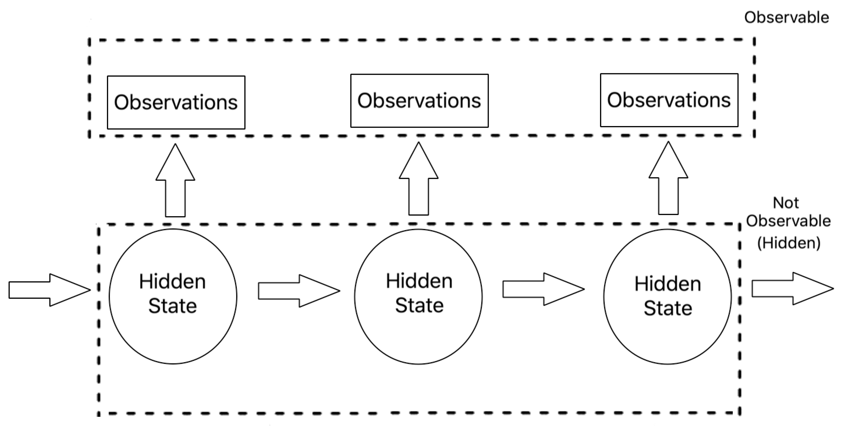
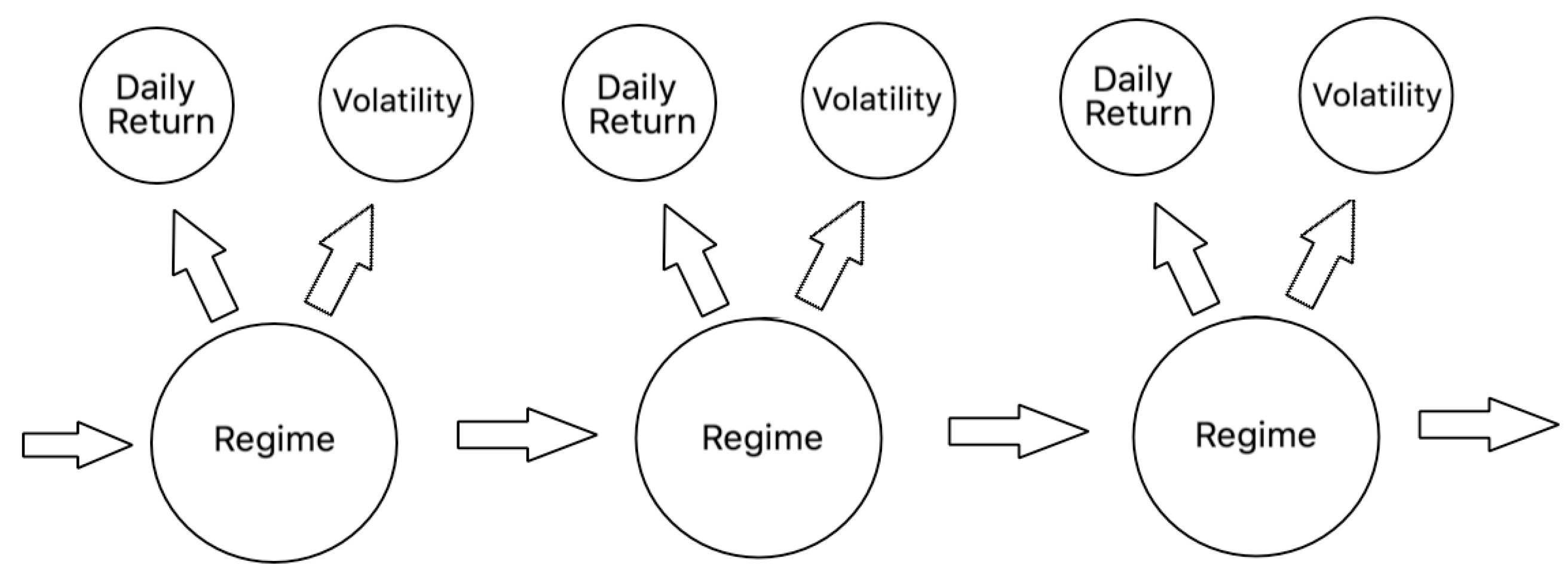
3.2. Hidden Markov Model
3.2.1. Model Description
HMMs are stochastic probabilistic models that aims to model a system as a Markov chain with hidden states and distinct transition and emission probabilities for each respective state. In this study, we use a Gaussian HMM which is a continuous HMM that models the probability distributions of its observations as Gaussian distributions.
The Gaussian HMM consists of four main parameters: the transition matrix A that delineates the probability of transition from one state to another, the observation probability distributions represented as and which contain the mean and variance for observations with respect to each respective hidden state, and as the vector of probabilities of initial starting states.
3.2.2. Model Application
When applying an HMM in the real world, there are three main subproblems that are associated with fitting the model.
- Estimate the probability of occurrence for the set of observations
- Determining the most optimal sequence of hidden states for the HMM given the set of observations
- Finding the optimal parameters A, , , and of the HMM.
The first problem can be solved by applying the forward algorithm. The forward algorithm is a dynamic programming algorithm that recursively computes the forward probabilities which calculates the probability of ending in a state given the prior observation sequence (). The algorithm does this by summing the probabilities of all of the various hidden state paths that can potentially generate the observation sequence.
The second problem can be solved by the Viterbi algorithm, a dynamic programming algorithm that “decodes” the observation sequence to find the most probable sequence of hidden states. The Viterbi algorithm recursively computes the most probable path through a sequence of states by storing the probability and state sequence of the most probable path at each point in time ().
Finally, in order to calibrate the parameters of the HMM, we can apply the Baum-Welch algorithm. The Baum-Welch algorithm makes use of the forward-backward algorithm, which is a dynamic programming method that computes the conditional distribution of observations for the hidden states in two passes (). In the first pass, the algorithm computes the forward probabilities as described in the forward algorithm, and in the second pass, the algorithm computes the backward probabilities which gives the probability of observing the rest of the observation sequence given a starting state. The results of both passes allow us to compute the probability of being in a state at any given point in time given the observation sequence, which is then iteratively used in an expectation-maximization fashion to move from our initial estimates of the parameters A, , , and to more probable estimates ().
Above in Table 1 and Table 2 you will find the results of our initial HMM parameters. These metrics were obtained by fitting the observations during the training period to the Gaussian HMM. These correspond to the aforementioned A and parameters of the HMM during the training period.
Table 1.
Initial state probabilities.
Table 2.
State transition probabilities.
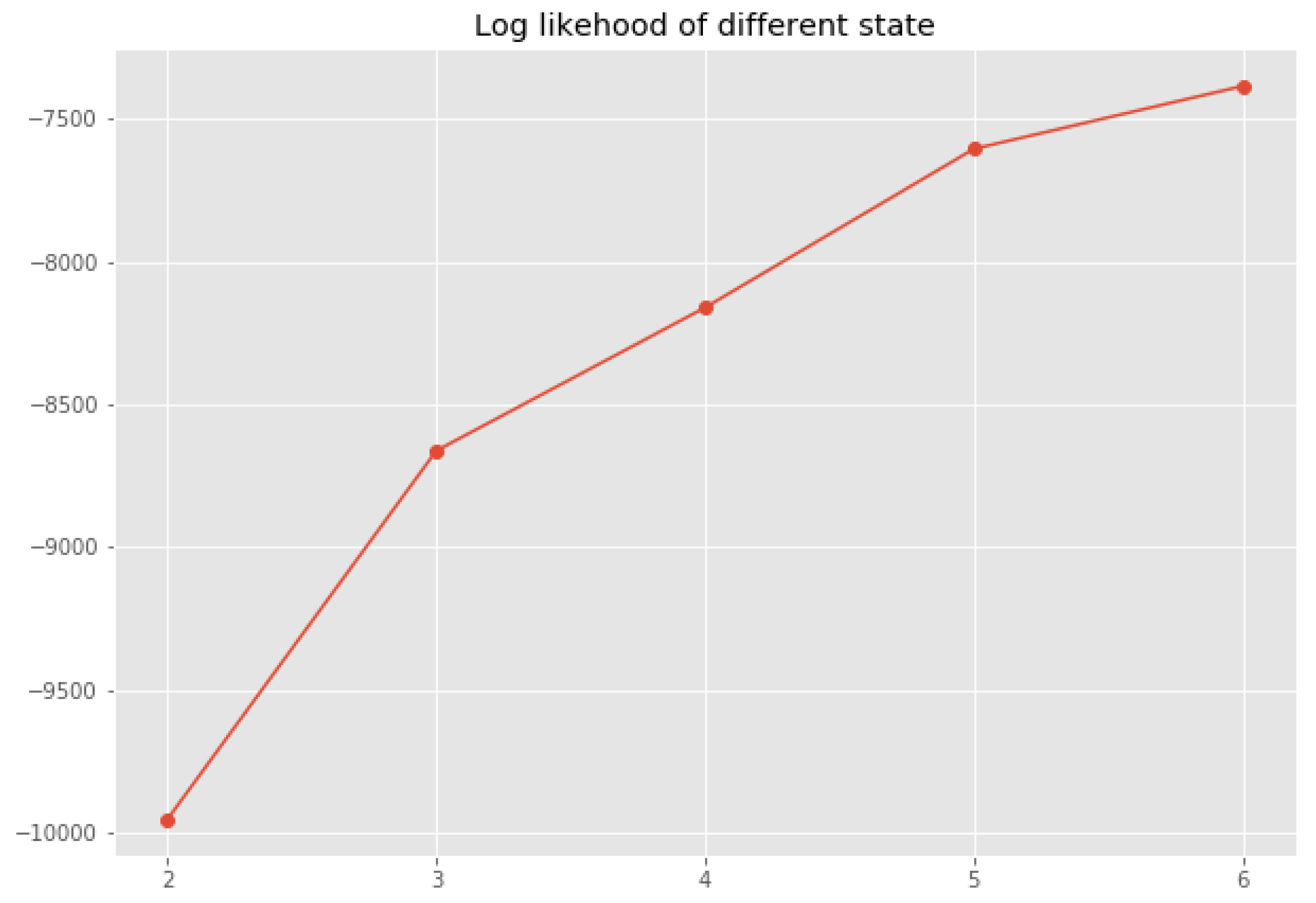
3.2.3. Model Configuration
In this study, we used the Gaussian hidden Markov model from the hmmlearn library1 in Python as the basis for our model. There are three primary parameters for our model that we define: the number of hidden states, the covariance type, and the threshold for the maximum number of iterations to perform for the expectation maximization algorithm.
An important consideration for determining the parameters for the HMM is the bias-variance tradeoff. Both the number of hidden states and the threshold for expectation maximization can influence the fit of the model. For the purposes of this study we settled on using three hidden states: representing periods including bull, bear, and neutral market regimes. We provide our analysis result in Figure 3 for selecting the number of regimes. The figure shows the model score, or the log-likelihood of the observations under an HMM that uses a different number of regimes. We have most improvement of our log-likelihood from a two-state model to a three-state model. In order to prevent overfitting as a way to balance the bias-variance trade-off, we decided to settle with a three-state model which also corresponds to our initial setting. We set the threshold for the number of EM iterations to 75 so our model yielded an average continuous regime period of approximately 12.5 days. As for the covariance type, we opted to use a full covariance matrix over a diagonal covariance matrix because we are forgoing the assumption that the elements in the feature vector are independent of each other. The advantage of the full covariance matrix over the diagonal matrix is the inclusion of cross-correlation between our features in our model at the cost of an increased number of parameters (). As shown in Figure 4, we classify approximately 10 years worth of S&P500 data into three discrete market regimes.
Figure 3.
Validating our selection of number of regimes.
Figure 4.
Diagram showing regime classification on the S&P500 ETF.
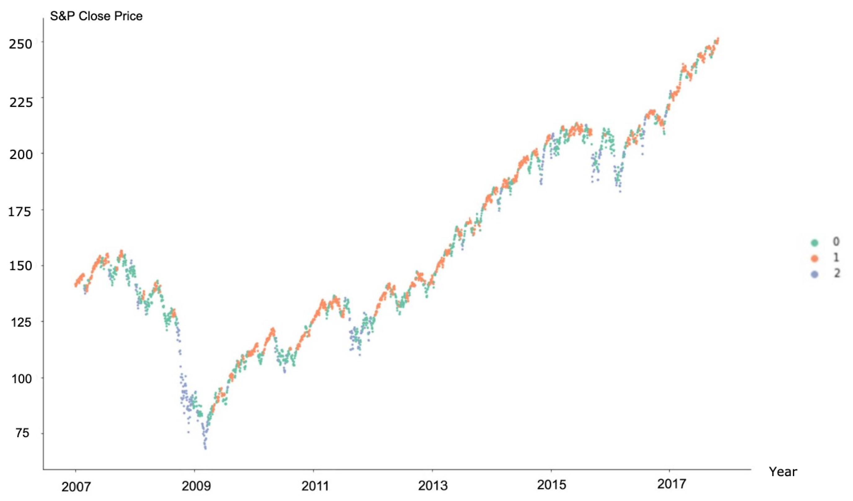
3.3. Regime Classification
From the volatility and daily return averages for the three respective hidden states classified by the HMM, we can see that one regime has the highest daily return with low volatility, one has nonetheless positive daily return but higher volatility, and the last one is characterized by a negative daily return with extremely high volatility. An important concern to address is the parity, or rather the lack thereof, between risk and return in the regimes. This can be attributed to the fact that we used both volatility and returns as observations to train the HMM, the HMM also tries to classify trading days based on the volatility behavior. Thus, the end result is that the unsupervised learning classifies three regimes each with a distinct pair of volatility/return patterns. The way we interpreted the end result was regime 1 being a steady bull-market regime, regime 2 being a highly-volatile bear market regime, and regime 0 being a sideways “kangaroo“ market regime. The observation metrics of each regime can be found in Table 3.
Table 3.
Regime analysis and breakdown.
3.4. Factor Models
For the purposes of this study, we utilized QuantConnect2 as our backtesting platform. We have built and tested six distinct factor models and observed their performance under each distinct regime within our training period.
3.4.1. Fama-French Three-Factor Model
The Fama-French three-factor model is a pricing model that aims to expand on and explain anomalies in the capital asset pricing model (CAPM) through suggesting that smaller size, excess return on the market, and high book-to-market equity are indicators of higher average returns (). Thus, we implemented a leveraged long/short model that selects stocks with the smallest market cap, lowest price-to-book ratio, and lowest price-to-earnings ratio. In this model we attempt to use price-to-book ratio in lieu of book-to-market ratio as the latter does not exist on QuantConnect. In addition, we also use price-to-earnings ratio as a proxy for excess return on the market.
3.4.2. Modified Fama–French Model
As for the modified Fama–French model, we closely follow the implementation of the Fama–French three-factor model described above, except we utilize price change within the past one month instead of price-to-earnings ratio to attempt to measure excess return on the market. In this case, we prioritize stocks that have shown the largest relative gain as a percentage of its stock price.
3.4.3. Carhart Four-Factor Model
The Carhart four-factor was a model that expands on the Fama-French three-factor model proposed by Mark Carhart, who observed that returns of mutual funds in the top decile in terms of performance tend to all be positively correlated with momentum while that of those in the bottom decile are highly, negatively correlated (). Thus, our implementation closely follows the implementation of the Fama–French three-factor model described above with an additional momentum factor. For the momentum factor, we choose to use the largest positive price change in the past month in an attempt to measure and observe the effect of short-term momentum in stock-picking.
3.4.4. Value
In this factor model, we aim to select high-value stocks that have the potential for stock price growth. We use dividend-per-share, book-value-per-share, and high free cash flow as a metric for value while using negative stock price changes to find a stock that will mean-revert and grow. Thus, we implemented a long-only model that selects stock based on highest dividend-per-share, highest book-value-per-share, highest free cash flow yield, and least or most negative stock price change in the past 1 month.
3.4.5. AQR Factor Model
In this factor model, we aim to capture the alpha described in stocks based on factors that pertain to quality, value, and momentum. shows that stocks with the aforementioned factors tend to generally outperform the market by delivering higher returns with lower risk. We emulate the concepts embodied by the models described by Frazzini by using a leveraged long/short model that selects stocks with the highest ratio of book-value-per-share to price, largest operating-income-to-revenue ratio, and largest or most positive stock price change in the past 1 month. By doing so, we aim to incorporate the factors of value, quality, and momentum respectively into our stock selection process.
3.4.6. S&P500 ETF
The Standard&Poors 500 index is a stock market index that aims to track the performance of 500 large-cap companies in the United States. It is often used as a benchmark for general market performance and conditions in the United States. For the S&P500, we simply pulled data for its ETF from Yahoo Finance to get its historical performance. For simplification purposes, we considered the S&P500 etf it’s own long-only “model”. This serves as a general benchmark for the performance of other factor models and is also used to signal -market conditions.
After performing regime classification with our HMM for the historical data, we are able to evaluate the quality of our factor models in these distinct regimes. We utilize the average daily return within the regime as well as the standard deviation of the daily returns to compute the Sharpe ratio, which we in turn use as a metric for quality for each respective factor model. For the computation of the Sharpe ratio, we subtract the risk-free rate from the model returns and divide it by the standard deviation of the excess returns.
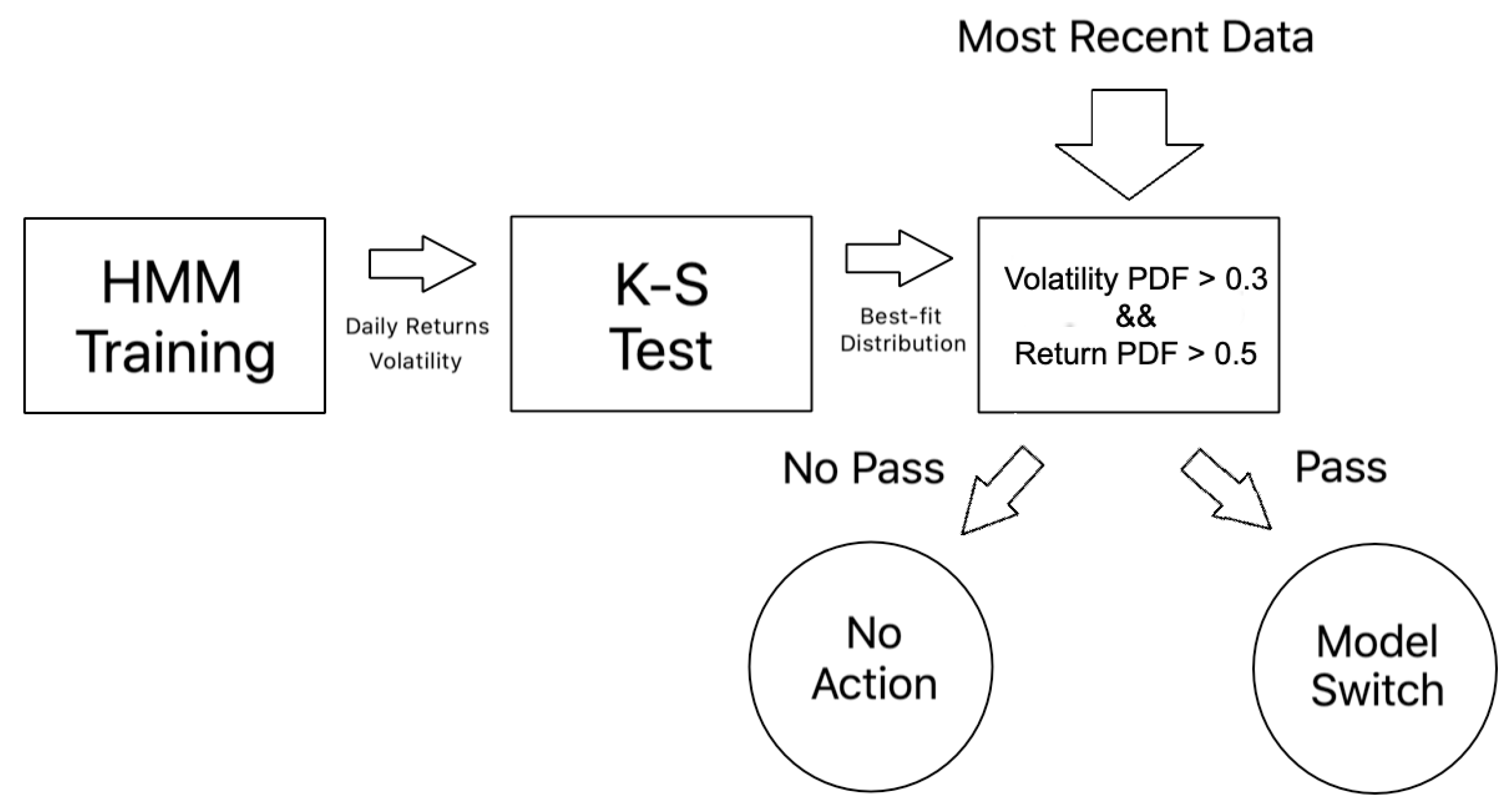
3.5. Trading Model Implementation
3.5.1. Model Training
When the model is trading live, it’s important for our algorithm to retrain the HMM so judgments on regime switches and regime detection are not based on past, outdated data. Thus, we implemented a sliding window methodology that retrains the model every day prior to market open on the most recent 2707 days worth of daily return and volatility data. Despite the continuous retraining of the model, we maintain the same definitions for the classification of regimes: the regime with the lowest or most negative returns, which typically also has the highest volatility, is the “bear” regime and the regime with the highest return is the “bull” regime. If we judge that a regime switch has occurred with a probability that exceeds a certain confidence interval, the model will switch to the other corresponding factor model.
3.5.2. Regime Detection
Once we have the trained HMM, we need to design a mechanism that serves as the aforementioned confidence interval for judging whether a regime switch has occurred. In using the GaussianHMM API from hmmlearn we operate under the assumption that the observation probability distributions for volatility and daily returns are normally distributed. However, in the mechanism we designed for regime detection, we analyzeg regime observations independently. Thus, as can be observed in Figure 5, we utilize the Kolmogorov-Smirnov test to fit the observations to one of many common distributions including normal, lognormal, pareto, gamma, beta and exponential. With new daily returns and volatility values, we are then able to use the probability density function (PDF) of the fitted distribution to compare the likelihood we are currently in each respective regime in relative terms. Finally, if our estimation of our confidence interval exceeds a certain threshold, in other words, if both the PDF of the volatility is greater than 0.3 and the PDF of the daily returns is greater than 0.5, the model concludes that we are in that respective regime and correspondingly switches to a factor model that historically performs well in those conditions.
Figure 5.
Diagram overview of our trading model.
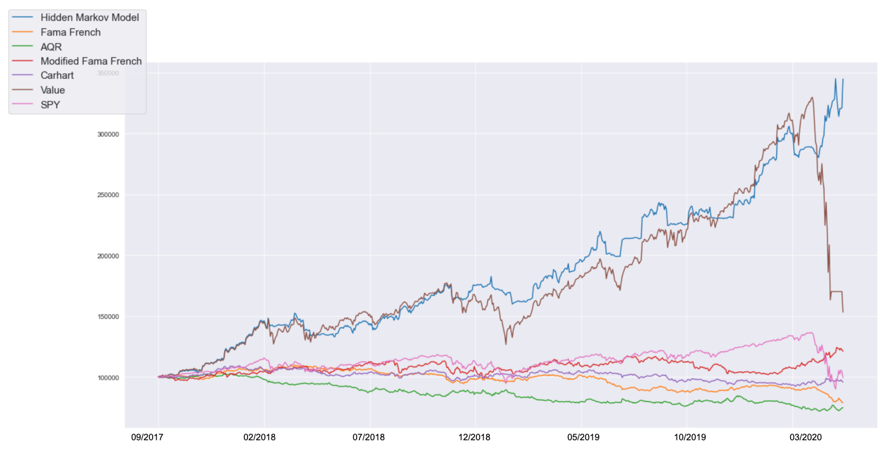
4. Empirical Analysis
In this section, we compare our HMM model with S&P500 and four factor models mentioned above. In order to conduct a fair comparison, we select four performance measurements: Sharpe ratio, information ratio, Treynor ratio, and the Treynor–Mazuy measurement.
4.1. Sharpe Ratio
The Sharpe ratio is a measure of risk-adjusted return for a security or portfolio. It was initially proposed to measure the average excess return per unit of risk with risk defined as the volatility of the excess return (). The Sharpe ratio helps explain whether the portfolio’s excess return is due to consistent intelligent decision-making or from taking on excessive risk, which can allow us to verify the effectiveness of our strategy.
where is return of portfolio, is risk-free rate, and is standard deviation of portfolio’s excess return. In this study, we considered the 10-year US treasury bond as our risk-free rate for the computation of the annualized Sharpe ratio.
4.2. Information Ratio
The information ratio (IR) is a measurement for the effectiveness of portfolio management relative to a benchmark index. It is defined as the ratio of the excess return over benchmark to the tracking error of the portfolio (). The tracking error can be understood as the skill of the portfolio manager since it is the consistency of the excess return. As a result, we use information ratio for the purpose of comparing the overall effectiveness of each portfolio. The magnitude of the value of the information ratio determines the consistency and efficiency of the performance.
where is return of portfolio, is the return of benchmark, and is the tracking error, or the standard deviation of the difference between the portfolios return and the benchmarks return. In this study, we use the return of S&P 500 as our benchmark return. If IR is positive, it means the portfolio management methodology efficiently processes the information and converts it into excess return.
4.3. Treynor Ratio
The Treynor ratio, similar to the Sharpe ratio, aims to measure the returns of a portfolio relative to the risk profile. However, the Treynor ratio differs in the way it defines risk. Rather than using the standard deviation of returns as a metric for volatility and risk by proxy, it utilizes the beta coefficient of the portfolio to quantify the systematic risk of the portfolio (). Beta, a measure of the non-diversifiable risk of a portfolio to the market, is defined as the covariance between portfolio returns and market returns divided by the variance of the market returns (). Thus, the higher the ratio the more compensation we have from bearing systematic risk to beta.
where is return of portfolio, is risk-free rate, and the beta of the portfolio. In this study, we report the annualized Treynor ratio.
4.4. Treynor-Mazuy Measurement
In order to show that our regime-switching HMM model indeed introduces market timing skill to our investment methodologies, we also verify it by utilizing Treynor-Mazuy measurement. The Treynor-Mazuy measurement is a quadratic performance measurement model based on CAPM that aims to measure the timing ability of portfolio managers and their ability to “outguess” the market (). The magnitude of the Treynor–Mazuy Measure depends primarily on two variables: portfolio returns and the variability of its risk sensitivities. For clarity, we present this measurement by showing the decomposition of excess return using the Treynor-Mazuy method.
where is excess return of portfolio, is market risk premium, is stock selection ability, is the beta coefficient of the portfolio, is market timing performance, and is the noise. In the mathematical sense, represents the curvature of the regression line obtained, which is desired by portfolio management since a positive value indicates that the portfolio returns are a convex function of market returns; the portfolio will gain more when the market goes up and lose less when the contrary occurs (). As a result, a significant and positive value demonstrates strong market timing ability in portfolio management ().
4.5. Evaluations
Table 4 summarizes the quantitative results of our experiment. As one can observe from Figure 6, the HMM model has higher returns and both a higher Sharpe ratio and a higher Treynor ratio when compared to the rest of the other models. This signifies that not only does the model deliver better-annualized returns as displayed in Table 5, the HMM model also generates better risk-adjusted returns when we account for both systematic market risk and volatility of returns as can be seen in Table 6 and Table 7. As for the information ratio, the HMM model performs well relatively and absolutely, signifying that the systematic portfolio management methodology we designed is effective. It has a higher IR value than that of all the other models and surpasses 1, which is commonly used as a benchmark. As for market timing ability with respect to the Treynor–Mazuy measurement, despite the relatively better results of our model, the Treynor-Mazuy coefficients in all of the models are not statistically significant enough. It corresponds to the fact that the risk exposures of our models are distinct from market risk, thus the market risk premium used in the Treynor–Mazuy cannot sufficiently explain the timing ability of our model. In order to validate whether our HMM model did provide superior performance, we ran a regression which takes HMM return as dependent variable and common factors as independent variables. The result is shown in Table 8. As we can see, even excluding the exposure of common factors3 we use in investment strategies, our HMM model still generate a significant abnormal return for approximately 2% annually.
Table 4.
Portfolio performance benchmarks for each model.
Figure 6.
Equity curve during testing period for each factor model.
Table 5.
Average regime return for each model less the risk-free rate.
Table 6.
Standard deviation of regime return for each model.
Table 7.
Regime Sharpe ratio for each model.
Table 8.
Regression result of 95% confidence level.
4.6. Qualitative Considerations
It’s important to recognize that the HMM regime-switching model essentially provides a methodology of conditionally switching the portfolio’s factor exposure and by proxy, style risk as well. This experiment empirically proves that such a model can improve your risk-adjusted returns through factor timing, a practice that entails exposing the portfolio to certain factors at times when those factors will deliver above-average returns (). In addition to factor timing, regime-switching models offer market timing skills to enhance investment performance. For instance, Dapena () relied on an HMM regime-switching model to determine risk-on and risk-off states for making active investment decisions. () used an HMM to time the individual asset and construct an asset allocation portfolio. In our paper, we provide a new methodology that delivers higher returns and results in better performance metrics by combining multiple investing models and rotating between these models through regime detection. As one can observe from the results in Figure 6, the HMM trading model performs more poorly than the value factor model during bull market runs. However, during market downturns like in December 2018 and March 2020, the HMM trading model switches from the twice-leveraged long-only value model to a market-neutral Fama French model which shields the portfolio from the drawdown it otherwise would have experienced.
5. Conclusions
Akin to results obtained by (), we can observe that using a hidden Markov model for asset allocation can prove to yield superior portfolio results. As one can observe from the previous section, our HMM that rotates between two-factor models yielded performance results superior to that of either factor model on which it is based. However, one important consideration for such a mode of investing is that even with an HMM rotating across different factor models, portfolio returns and performance will still be heavily contingent on and limited by the inherent quality of the factor models the HMM is based on. The HMM can only be thought of as a tool to diversify investment to a pool of factor models in order to hedge against market trends or macroeconomic regimes that various models might be particularly susceptible to.
Additionally, there are definitely further developments that can be made to the model we introduced in this paper. For instance, in order to maintain a balance between model bias and variance, we didn’t dive as deeply into model parameter optimization in order to prevent overfitting. We can definitely conduct more research on optimizations that can be made with respect to the parameters of the HMM. Furthermore, one can also improve the quality and increase the number of factor models while increasing the number of regimes their HMM classifies to potentially create superior and more versatile investing models.
Author Contributions
All authors made significant contributions to the paper. Conceptualization, M.W. and Y.-H.L.; methodology, M.W.; software, M.W.; validation, M.W. and Y.-H.L.; formal analysis, M.W. and Y.-H.L.; investigation, M.W. and Y.-H.L.; resources, M.W. and I.M.; data curation, M.W.; writing—original draft preparation, M.W., Y.-H.L., and I.M.; writing–review and editing, M.W. and I.M.; visualization, M.W. All authors have read and agreed to the published version of the manuscript.
Funding
This research received funding from Northwestern University for the submission of this paper.
Acknowledgments
We acknowledge the contribution, support, and guidance that Professor Ilya Mikhelson from Northwestern University provided for this research. Without him, this research would not have been possible.
Conflicts of Interest
The author declares no conflict of interest.
References
- Asness, Clifford S., Andrea Frazzini, and Lasse H. Pedersen. 2014. Quality minus junk. SSRN Electronic Journal 24: 34–112. [Google Scholar]
- Ammann, Manuel, and Michael Verhofen. 2006. The Effect of Market Regimes on Style Allocation. Financial Markets and Portfolio Management 20: 309–37. [Google Scholar] [CrossRef]
- Ang, Andrew, Geert Bekaert, and Min Wei. 2008. The Term Structure of Real Rates and Expected Inflation. Journal of Finance 63: 797–849. [Google Scholar] [CrossRef]
- Ang, Andrew, and Geert Bekaert. 2004. How Do Regimes Affect Asset Allocation. Financial Analysts Journal 60: 86–99. [Google Scholar] [CrossRef]
- Asness, Clifford S. 2016. The Siren Song of Factor Timing. Journal of Portfolio Management. [Google Scholar] [CrossRef]
- Baum, Leonard E., and John Alonzo Eagon. 1967. An Inequality with Applications to Statistical Estimation for Probabilistic Functions of a Markov Process and to a Model for Ecology. Bulletin of the American Mathematical Society 73: 360–63. [Google Scholar] [CrossRef]
- Baum, Leonard E., Ted Petrie, George Soules, and Norman Weiss. 1970. A Maximization Technique Occurring in the Statistical Analysis of Probabilistic Functions of Markov Chains. The Annals of Mathemtatical Statistics 41: 164–71. [Google Scholar] [CrossRef]
- Bender, Jennifer, Remy Briand, Dimitris Melas, and Raman Aylur Subramanian. 2013. Foundations of Factor Investing. MSCI Research Insight. [Google Scholar] [CrossRef]
- Carhart, Mark M. 1997. On Persistence in Mutual Fund Performance. The Journal of Finance 52: 57–82. [Google Scholar] [CrossRef]
- Chen, Jun, and Edward Tsang. 2018. Classification of Normal and Abnormal Regimes in Financial Markets. Algorithms 11: 202. [Google Scholar] [CrossRef]
- Clarke, Roger, Harindra de Silva, and Steven Thorley. 2001. Portfolio Constraints and The Fundamental Law of Active Management. SSRN Electronic Journal 58: 48–66. [Google Scholar] [CrossRef]
- Cont, Rama. 2005. Volatility Clustering in Financial Markets: Empirical Facts and Agent-Based Models. In Long Memory in Economics. Berlin: Springer. [Google Scholar]
- Dapena, José P., Juan Andrés Serur, and Julián R. Siri. 2019. Risk On-Risk Off: A Regime Switching Model for Active Portfolio Management. Buenos Aires: Universidad del CEMA. [Google Scholar]
- Daniel, Kent, and Tobias Moskowitz. 2014. Momentum Crashes. SSRN Electronic Journal 122: 221–47. [Google Scholar]
- Fama, Eugene F., and Kenneth R. French. 1993. Common Risk Factors in the Returns on Stocks and Bonds. Journal of Financial Economics 33: 3–56. [Google Scholar] [CrossRef]
- Fama, Eugene F., and Kenneth R. French. 2004. The Capital Asset Pricing Model: Theory and Evidence. Journal of Economic Perspectives 18: 25–46. [Google Scholar] [CrossRef]
- Frazzini, Andrea, and Lasse Heje Pedersen. 2014. Betting against Beta. Journal of Financial Economics 111: 1–25. [Google Scholar] [CrossRef]
- Frazzini, Andrea, Ronen Israel, Tobias J. Moskowitz, and Robert Novy-Marx. 2013. A New Core Equity Paradigm. AQR Research White Papers. Greenwich: AQR Capital Management. [Google Scholar]
- Gibbons, Joel Clarke. 2010. The S&P500 Universe: Trend and Volatility Regimes. The Journal of Index Investing 1: 85–91. [Google Scholar]
- Hamilton, James D. 1989. A New Approach to the Economic Analysis of Nonstationary Time Series and the Business Cycle. Econometrica 57: 357–84. [Google Scholar] [CrossRef]
- Hwang, Soosung, and Mark Salmon. 2001. An Analysis of Performance Measures Using Copulae. Oxford: Butterworth-Heinemann. [Google Scholar]
- Ilmanen, Antti S., Ronen Israel, Tobias J. Moskowitz, Ashwin K. Thapar, and Franklin Wang. 2019. Factor Premia and Factor Timing: A Century of Evidence. SSRN Electronic Journal. [Google Scholar] [CrossRef]
- Kim, Chang-Jin, and Charles R. Nelson. 2017. State-Space Models with Regime Switching. Cambridge: MIT Press. [Google Scholar]
- Kim, Eun-Chong, Han-Wook Jeong, and Nak-Young Lee. 2019. Global Asset Allocation Strategy Using a Hidden Markov Model. Journal of Risk and Financial Management 12: 168. [Google Scholar] [CrossRef]
- Kritzman, Mark, Sébastien Page, and David Turkington. 2012. Regime Shifts: Implications for Dynamic Strategies. Financial Analysts Journal 68: 22–39. [Google Scholar] [CrossRef]
- Gales, Mark J. F. 1999. Semi-tied Covariance Matrices for Hidden Markov Models. IEEE Transactions on Speech and Audio Processing 7: 272–81. [Google Scholar] [CrossRef]
- Hassan, Md Rafiul, and Baikunth Nath. 2005. Stock market forecasting using hidden Markov model: A new approach. Paper presented at 5th International Conference on Intelligent Systems Design and Applications, Auburn, WA, USA, December 3–5; pp. 192–196. [Google Scholar]
- Nguyen, Nguyet, and Dung Nguyen. 2015. Hidden Markov Model for Stock Selection. Risks 3: 455–73. [Google Scholar] [CrossRef]
- Paramita, V. Santi. 2015. Testing Treynor-Mazuy Conditional Model in Bull and Bear Market. Society of Interdisciplinary Business Research 4: 208–19. [Google Scholar]
- Rabiner, Lawrence R. 1989. A Tutorial on Hidden Markov Models and Selected Applications in Speech Recognition. Proceedings of the IEEE 77: 257–86. [Google Scholar] [CrossRef]
- Raffinot, Thomas. 2007. Hidden Markov Models Fundamentals. CS229 Section Notes 1. Available online: http://cs229.stanford.edu/section/cs229-hmm.pdf (accessed on 7 September 2020).
- Ramage, Daniel. 2007. Time-Varying Risk Premiums and Economic Cycles. SSRN Electronic Journal. [Google Scholar] [CrossRef]
- Ross, Stephen A. 1976. The Arbitrage Theory of Capital Asset Pricing. Journal of Economic Theory 13: 341–60. [Google Scholar] [CrossRef]
- Sharpe, William F. 1966. Mutual Fund Performance. Journal of Business 34: 119–38. [Google Scholar] [CrossRef]
- Treynor, Jack, and Kay Mazuy. 1966. Can Mutual Funds Outguess the Market? Harvard Business Review 44: 131–6. [Google Scholar]
- Treynor, Jack. 1965. How to Rate Management of Investment Funds. Harvard Business Review 41: 63–75. [Google Scholar]
- Viterbi, Andrew. 1967. Error Bounds for Convolutional Codes and An Asymptotically Optimum Decoding Algorithm. IEEE Transactions on Information Theory 13: 260–69. [Google Scholar] [CrossRef]
- Vo, Huyh Thanh, and Raimond Maurer. 2013. Dynamic Asset Allocation with Regime Shifts and Long Horizon CVaR-Constraints. SSRN Electronic Journal. [Google Scholar] [CrossRef]
- Yuan, Yuan, and Mitra Gautam. 2019. Market Regime Identification Using Hidden Markov Models. SSRN Electronic Journal. [Google Scholar] [CrossRef]
| 1. | Open-sourced HMM library https://hmmlearn.readthedocs.io/. |
| 2. | Free algorithmic backtesting and trading tool https://www.quantconnect.com/. |
| 3. | We obtain MKT, SMB, HML, MOM from Ken French’s data library: http://mba.tuck.dartmouth.edu/pages/faculty/ken.french/data_library.html; QMJ data comes from Andrea Frazzin’s library: http://www.econ.yale.edu/~af227/data_library.htm. |
Publisher’s Note: MDPI stays neutral with regard to jurisdictional claims in published maps and institutional affiliations. |
© 2020 by the authors. Licensee MDPI, Basel, Switzerland. This article is an open access article distributed under the terms and conditions of the Creative Commons Attribution (CC BY) license (http://creativecommons.org/licenses/by/4.0/).