Overreaction in the REITs Market: New Evidence from Quantile Autoregression Approach


Abstract
1. Introduction
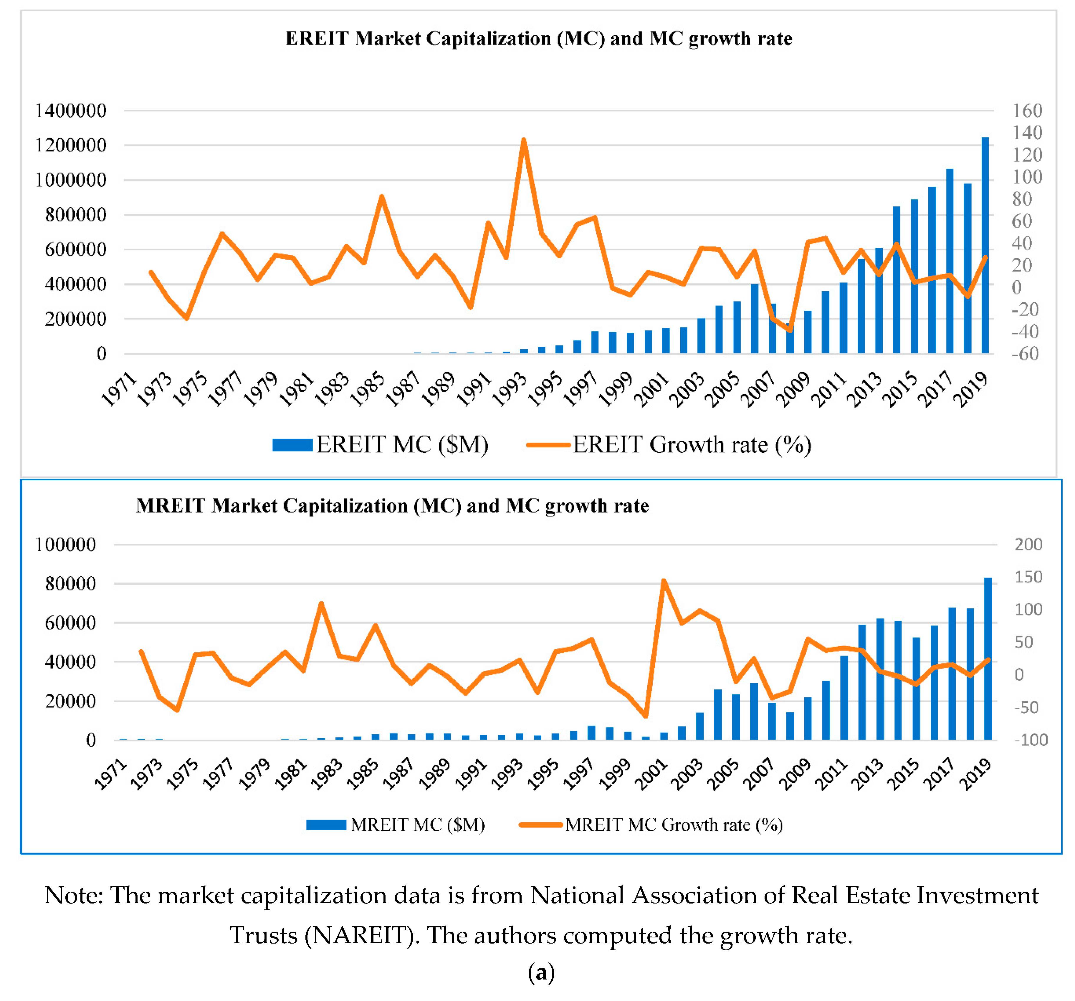
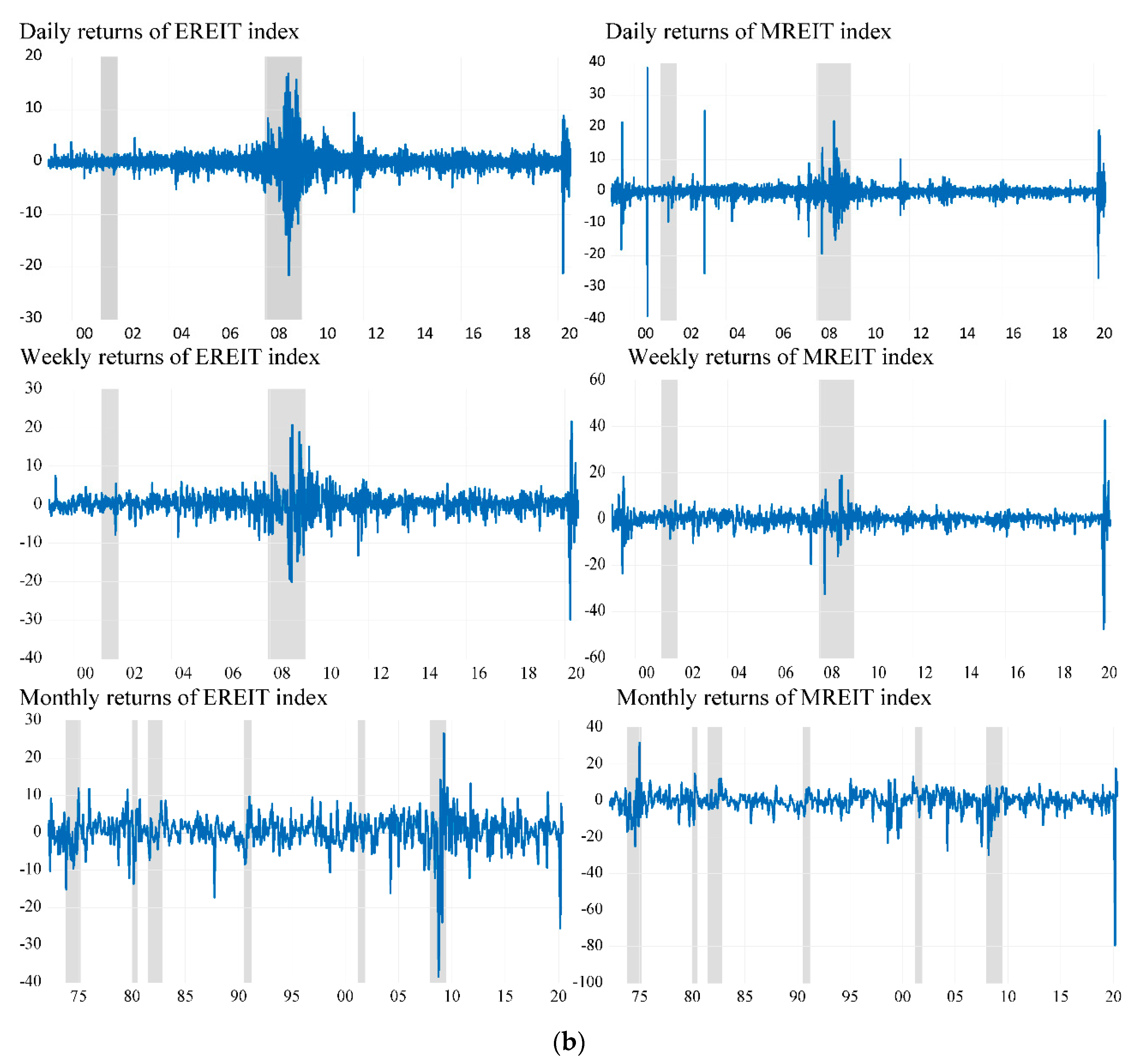
2. Data Sources and Data Characterization
3. Econometric Model
- (1)
- (there is no recession-specific change in the average degree of dependence.) Rejecting the null hypothesis implies that the degree of return dependency, on average, changes during the crisis period.
- (2)
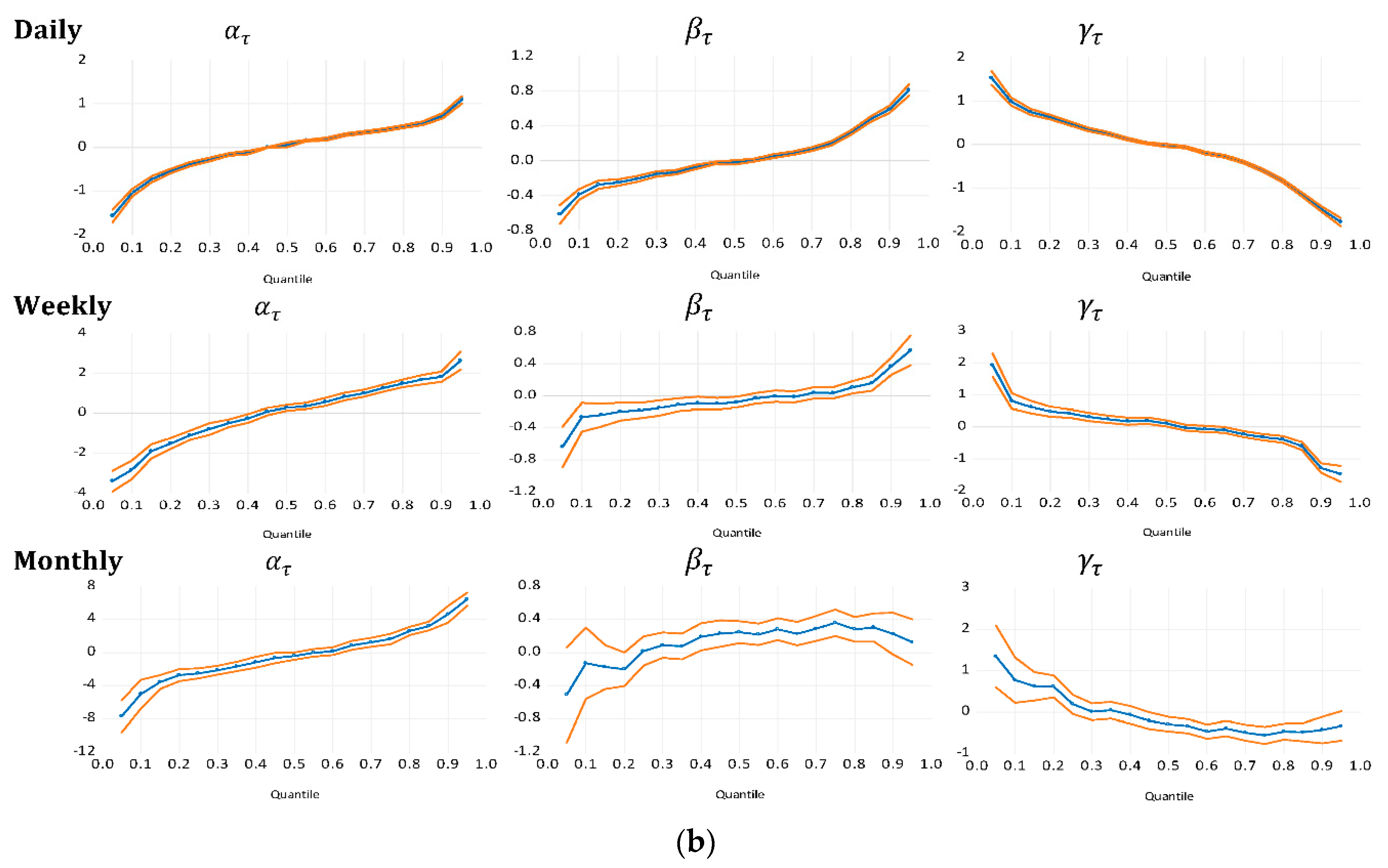
- (there is no recession-specific change in the structure of dependency or is not constant across all quantiles). Rejection of the null means that dependence structure changes during recession periods relative to non-recession periods.
4. Empirical Results
Additional Analysis
5. Summary and Conclusions
Author Contributions
Funding
Conflicts of Interest
References
- Aguilar, Mike, Walter I. Boudry, and Robert A. Connolly. 2018. The dynamics of REIT pricing efficiency. Real Estate Economics 46: 251–83. [Google Scholar] [CrossRef]
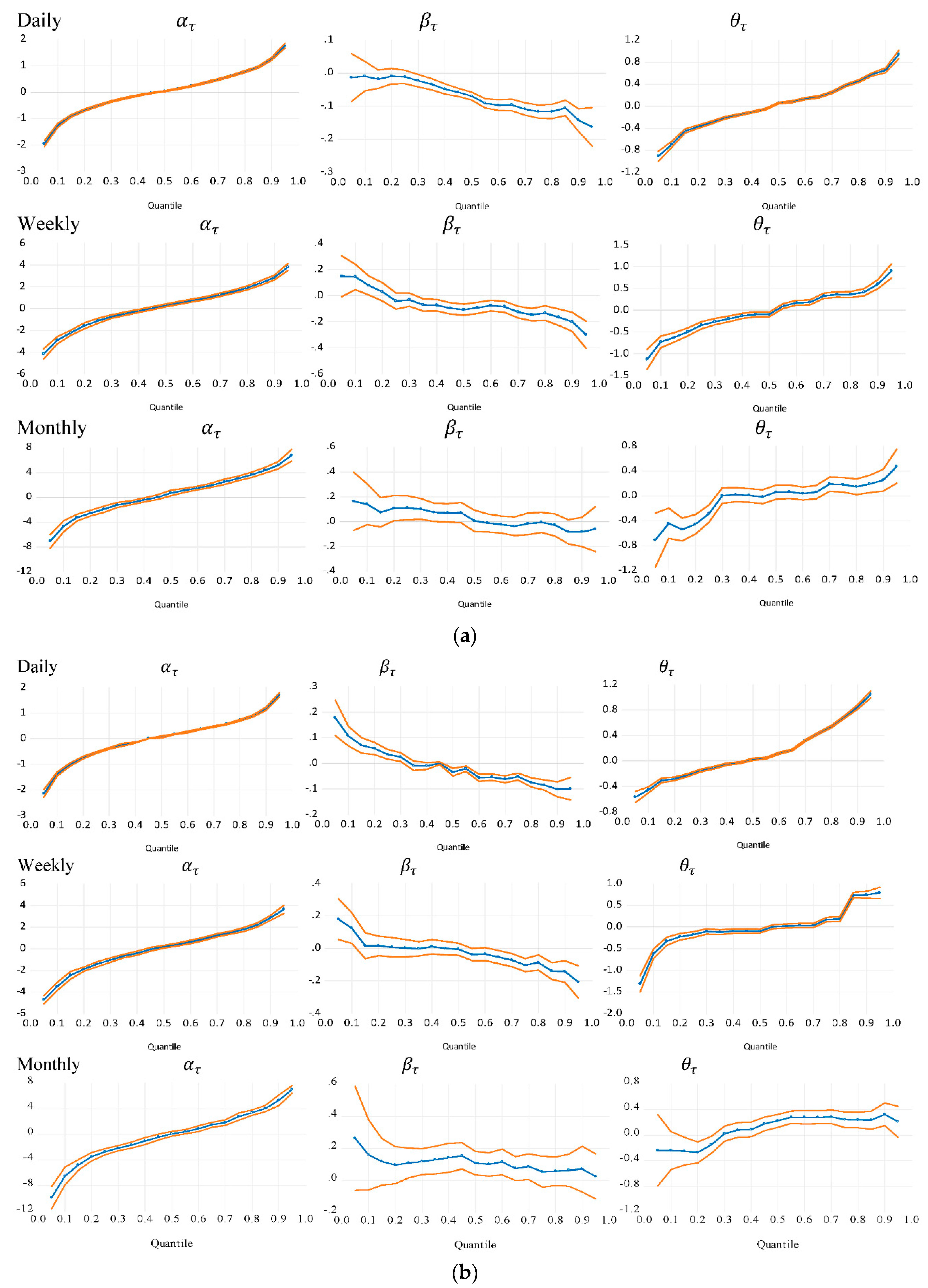
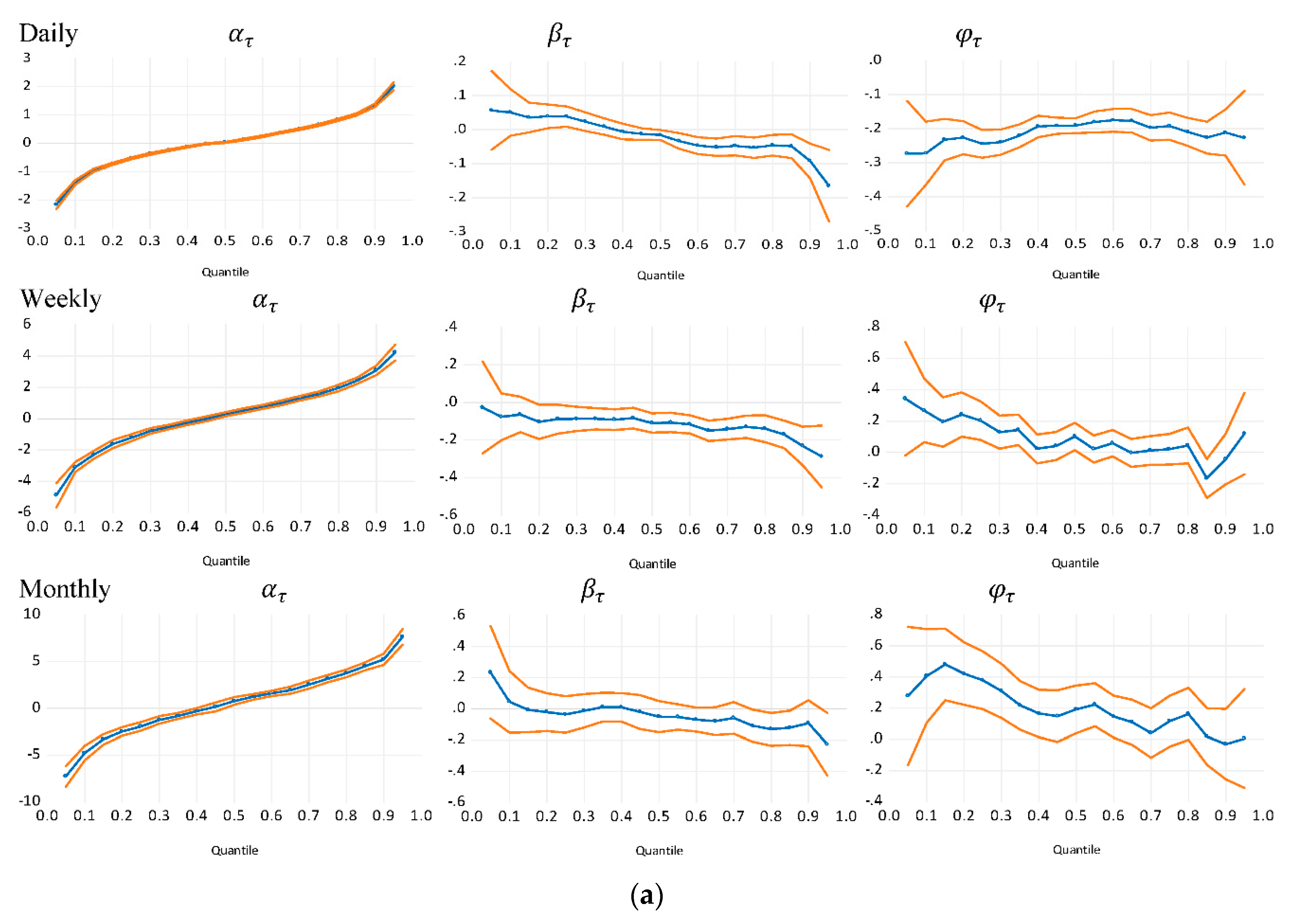
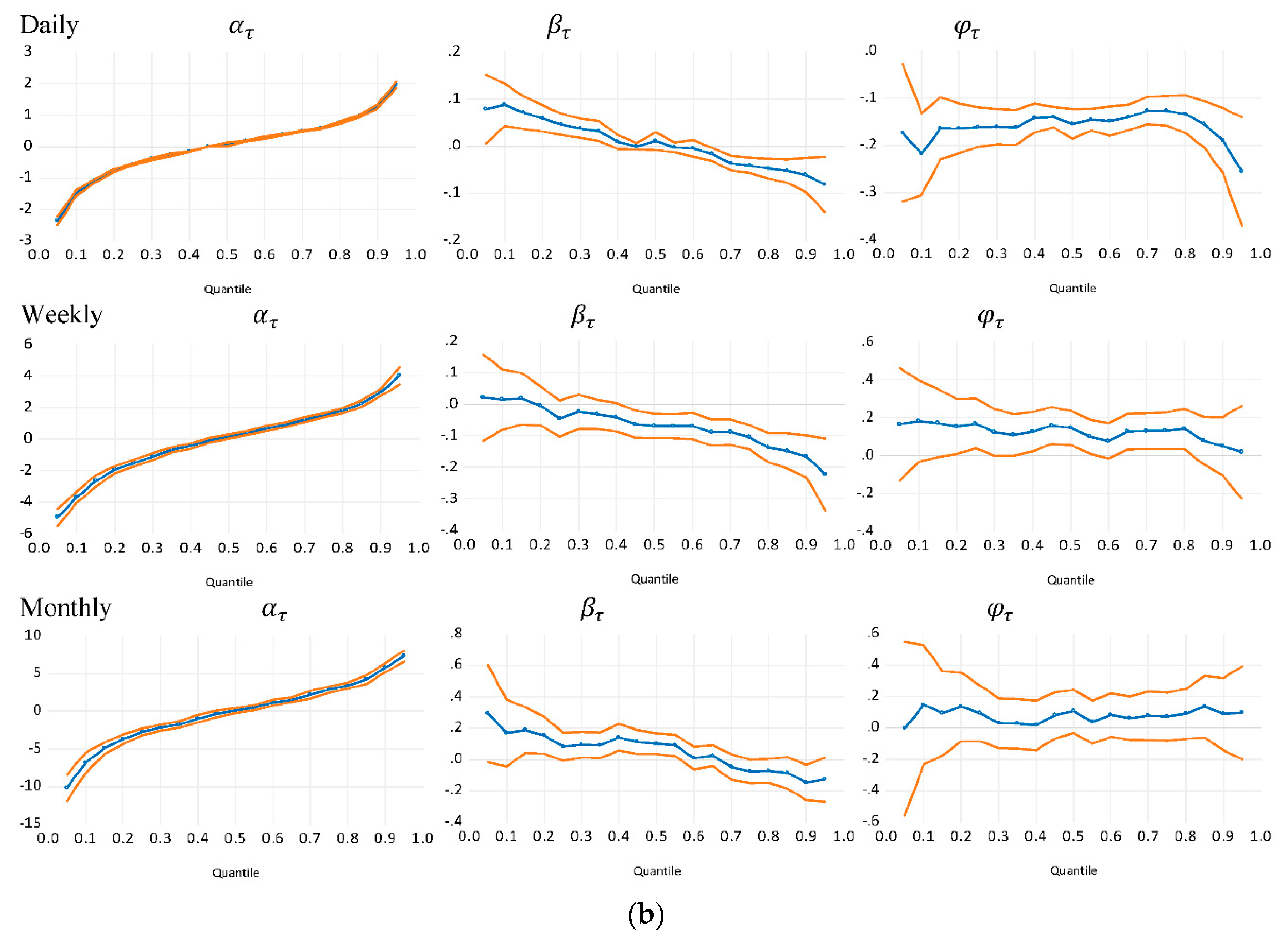
- Anderson, Robert M., Kyong Shik Eom, Sang Buhm Hahn, and Jong-Ho Park. 2013. Autocorrelation and partial price adjustment. Journal of Empirical Finance 24: 78–93. [Google Scholar] [CrossRef]
- Assaf, Ata. 2015. Long memory and level shifts in REITs return and volatility. International Review of Financial Analysis 42: 172–82. [Google Scholar] [CrossRef]
- Barberis, Nicholas, Andrei Shleifer, and Robert Vishny. 1998. A model of investor sentiment. Journal of Financial Economics 49: 307–43. [Google Scholar] [CrossRef]
- Basu, Sudipta. 1997. The conservatism principle and the asymmetric timeliness of earnings. Journal of Accounting and Economics 24: 3–37. [Google Scholar] [CrossRef]
- Baur, Dirk G. 2013. The structure and degree of dependence: A quantile regression approach. Journal of Banking & Finance 37: 786–98. [Google Scholar]
- Baur, Dirk G., Thomas Dimpfl, and Robert C. Jung. 2012. Stock return autocorrelations revisited: A quantile regression approach. Journal of Empirical Finance 19: 254–65. [Google Scholar] [CrossRef]
- Black, Fischer. 1989. Mean Reversion and Consumption Smoothing. Working Paper 2946. Cambridge, UK: NBER. [Google Scholar]
- Brennan, Thomas J., and Andrew W. Lo. 2011. The Origin of Behavior. Quarterly Journal of Finance 1: 55–108. [Google Scholar] [CrossRef]
- Buchinsky, Moshe. 1995. Estimating the asymptotic covariance matrix for quantile regression models: A Monte Carlo study. Journal of Econometrics 68: 303–38. [Google Scholar] [CrossRef]
- Campbell, John Y., Sanford J. Grossman, and Jiang Wang. 1993. Trading Volume and Serial Correlation in Stock Returns. Quarterly Journal of Economics 108: 905–39. [Google Scholar] [CrossRef]
- Campbell, John Y., John J. Champbell, John W. Campbell, Andrew W. Lo, Andrew W. Lo, and A. Craig MacKinlay. 1997. The Econometrics of Financial Markets. Princeton: Princeton University Press. [Google Scholar]
- Chandrashekaran, Vinod. 1999. Time-Series Properties and Diversification Benefits of REIT Returns. The Journal of Real Estate Research 17: 91–112. [Google Scholar]
- Chevapatrakul, Thanaset, and Danilo V. Mascia. 2019. Detecting overreaction in the Bitcoin market: A quantile autoregression approach. Finance Research Letters 30: 371–77. [Google Scholar] [CrossRef]
- Chui, Andy C. W., Sheridan Titman, and KC John Wei. 2003. Intra-industry momentum: The case of REITs. Journal of Financial Markets 6: 363–87. [Google Scholar] [CrossRef]
- Clayton, Jim, and Greg MacKinnon. 2003. The relative importance of stock, bond, and real estate factors in explaining REIT returns. The Journal of Real Estate Finance and Economics 27: 39–60. [Google Scholar] [CrossRef]
- Copeland, Thomas E. 1976. A model of assets trading under the assumption of sequential information arrival. Journal of Finance 31: 1149–68. [Google Scholar] [CrossRef]
- Cotter, John, and Simon Stevenson. 2008. Modeling long memory in REITs. Real Estate Economics 36: 533–54. [Google Scholar] [CrossRef]
- Daniel, Kent, David Hirshleifer, and Avanidhar Subrahmanyam. 1998. Investor psychology and security market under- and over-reactions. Journal of Finance 53: 1839–86. [Google Scholar] [CrossRef]
- Escanciano, J. Carlos, and Ignacio N. Lobato. 2009. An automatic Portmanteau test for serial correlation. Journal of Econometrics 151: 140–49. [Google Scholar] [CrossRef]
- Faff, Robert W., and Michael D. McKenzie. 2007. The relationship between implied volatility and autocorrelation. International Journal of Managerial Finance 3: 191–96. [Google Scholar] [CrossRef]
- Feng, Zhilan, S. McKay Price, and C. Sirmans. 2011. An overview of equity real estate investment trusts (REITs): 1993–2009. Journal of Real Estate Literature 19: 307–43. [Google Scholar]
- Feng, Zhilan, S. McKay Price, and C. F. Sirmans. 2014. The relation between momentum and drift: Industry-level evidence from equity Real Estate Investment Trusts (REITs). Journal of Real Estate Research 36: 383–407. [Google Scholar] [CrossRef][Green Version]
- Glascock, John L., Chiuling Lu, and Raymond W. So. 2000. Further evidence on the integration of REIT, bond, and stock returns. The Journal of Real Estate Finance and Economics 20: 177–94. [Google Scholar] [CrossRef]
- Glosten, Lawrence R., Ravi Jagannathan, and David E. Runkle. 1993. On the relation between the expected value and the volatility of the nominal excess return on stocks. Journal of Finance 48: 1779–1801. [Google Scholar] [CrossRef]
- Goebel, Paul R., David M. Harrison, Jeffrey M. Mercer, and Ryan J. Whitby. 2013. REIT momentum and characteristic-related REIT returns. Journal of Real Estate Finance and Economics 47: 564–81. [Google Scholar] [CrossRef]
- Hao, Ying, Hsiang-Hui Chu, Kuan-Cheng Ko, and Lin Lin. 2016. Momentum strategies and investor sentiment in the REIT market. International Review of Finance 16: 41–71. [Google Scholar] [CrossRef]
- Ho, Kim Hin David, and Shea Jean Tay. 2016. REIT market efficiency through a binomial option pricing tree approach. Journal of Property Investment & Finance 34: 496–520. [Google Scholar]
- Holden, Craig W., and Avanidhar Subrahmanyam. 2002. News events, information acquisition, and serial correlation. Journal of Business 1: 1–32. [Google Scholar] [CrossRef]
- Hui, Eddie C. M., and Sheung-Chi Phillip Yam. 2014. Can we beat the “buy-and-hold” strategy? Analysis on European and American securitized real estate indices. International Journal of Strategic Property Management 18: 28–37. [Google Scholar] [CrossRef]
- Hui, E. C. M., J. A. Wright, and S. C. P. Yam. 2014. Calendar effects and real estate securities. Journal of Real Estate Finance and Economics 49: 91–115. [Google Scholar] [CrossRef]
- Hung, Szu-Yin Kathy, and John L. Glascock. 2008. Momentum profitability and market trend: Evidence from REITs. Journal of Real Estate Finance and Economics 37: 51–69. [Google Scholar] [CrossRef]
- Jennings, Robert H., Laura T. Starks, and John C. Fellingham. 1981. An equilibrium model of asset trading with sequential information arrival. Journal of Finance 36: 143–61. [Google Scholar] [CrossRef]
- Jirasakuldech, Benjamas, and John Knight. 2005. Efficiency in the market for REITs: Further evidence. Journal of Real Estate Portfolio Management 11: 123–32. [Google Scholar] [CrossRef]
- Karolyi, G. Andrew, and Anthony B. Sanders. 1998. The variation of economic risk premiums in real estate returns. The Journal of Real Estate Finance and Economics 17: 245–62. [Google Scholar] [CrossRef]
- Kleiman, Robert, James Payne, and Anandi Sahu. 2002. Random walks and market efficiency: Evidence from international real estate markets. Journal of Real Estate Research 24: 279–97. [Google Scholar]
- Koenker, Roger, and Gilbert Bassett, Jr. 1978. Regression quantiles. Econometrica 1: 33–50. [Google Scholar] [CrossRef]
- Koenker, Roger, and Gilbert Bassett, Jr. 1982. Robust tests for heteroscedasticity based on regression quantiles. Econometrica 50: 43–62. [Google Scholar] [CrossRef]
- Koenker, Roger, and Zhijie Xiao. 2006. Quantile autoregression. Journal of the American Statistical Association 101: 980–90. [Google Scholar] [CrossRef]
- Kuhle, James, and Jaime Alvayay. 2000. The efficiency of equity REIT prices. Journal of Real Estate Portfolio Management 6: 349–54. [Google Scholar]
- Lee, Ming-Long, and Kevin Chiang. 2004. Substitutability between equity REITs and mortgage REITs. Journal of Real Estate Research 26: 95–113. [Google Scholar]
- Lee, Ming-Te, M. L. Lee, Bang-Han Chiu, and Chyi Lin Lee. 2014. Do lunar phases affect US REIT returns? Investment Analysts Journal 43: 67–78. [Google Scholar] [CrossRef]
- Lehmann, Bruce N. 1990. Fads, Martingales, and Market Efficiency. The Quarterly Journal of Economics 105: 1–28. [Google Scholar] [CrossRef]
- Lewellen, Jonathan. 2002. Momentum and autocorrelation in stock returns. Review of Financial Studies 15: 533–64. [Google Scholar] [CrossRef]
- Li, Lili, Shan Leng, Jun Yang, and Mei Yu. 2016. Stock Market Autoregressive Dynamics: A Multinational Comparative Study with Quantile Regression. Mathematical Problems in Engineering 2016: 1285768. [Google Scholar] [CrossRef]
- Liow, Kim Hiang. 2009. Long-term memory in volatility: Some evidence from international securitized real estate markets. Journal of Real Estate Finance and Economics 39: 415–38. [Google Scholar] [CrossRef]
- Liu, Jian, Cheng Cheng, Xianglin Yang, Lizhao Yan, and Yongzeng Lai. 2019. Analysis of the efficiency of Hong Kong REITs market based on Hurst exponent. Physica A: Statistical Mechanics and Its Applications 534: 122035. [Google Scholar] [CrossRef]
- Ljung, Greta M., and George E. P. Box. 1978. On a measure of lack of fit in time series models. Biometrika 65: 297–303. [Google Scholar] [CrossRef]
- Lo, Andrew W. 2004. The adaptive markets hypothesis. Journal of Portfolio Management 30: 15–29. [Google Scholar] [CrossRef]
- Lo, Andrew W. 2017. Adaptive Markets: Financial Evolution at the Speed of Thought. Princeton: Princeton University Press. [Google Scholar]
- Lo, Andrew W., and A. Craig MacKinlay. 1990. When Are Contrarian Profits Due to Stock Market Overreaction? Review of Financial Studies 3: 175–205. [Google Scholar] [CrossRef]
- Mech, Timothy S. 1993. Portfolio return autocorrelation. Journal of Financial Economics 34: 307–44. [Google Scholar] [CrossRef]
- Mei, Jianping, and Bin Gao. 1995. Price reversal, transaction costs, and arbitrage profits in the real estate securities market. Journal of Real Estate Finance and Economics 11: 153–65. [Google Scholar] [CrossRef]
- Mull, Stephen R., and Luc A. Soenen. 1997. US REITs as an asset class in international investment portfolios. Financial Analysts Journal 53: 55–61. [Google Scholar] [CrossRef]
- Nelling, Edward, and Joseph Gyourko. 1998. The Predictability of Equity REIT Returns. Journal of Real Estate Research 16: 251–68. [Google Scholar]
- Nikolaou, Kleopatra. 2008. The behaviour of the real exchange rate: Evidence from regression quantiles. Journal of Banking & Finance 32: 664–79. [Google Scholar]
- Nofsinger, John R., and Richard W. Sias. 1999. Herding and feedback trading by institutional and individual investors. Journal of Finance 54: 2263–95. [Google Scholar] [CrossRef]
- Peterson, James D., and Cheng-Ho Hsieh. 1997. Do common risk factors in the returns on stocks and bonds explain returns on REITs? Real Estate Economics 25: 321–45. [Google Scholar] [CrossRef]
- Schindler, Felix. 2011. Market efficiency and return predictability in the emerging securitized real estate markets. Journal of Real Estate Literature 19: 111–50. [Google Scholar]
- Schindler, Felix, Nico Rottke, and Roland Füss. 2010. Testing the predictability and efficiency of securitized real estate markets. Journal of Real Estate Portfolio Management 16: 171–91. [Google Scholar] [CrossRef]
- Sentana, Enrique, and Sushil Wadhwani. 1992. Feedback traders and stock return autocorrelation: Evidence from a century of daily data. The Economic Journal 102: 415–25. [Google Scholar] [CrossRef]
- Shen, Jianfu, Eddie C. M. Hui, and Kwokyuen Fan. 2020. The Beta Anomaly in the REIT Market. Journal of Real Estate Finance and Economics, 1–23, in press. [Google Scholar] [CrossRef]
- Sias, Richard W., and Laura T. Starks. 1997. Return autocorrelation and institutional investors. Journal of Financial Economics 46: 103–31. [Google Scholar] [CrossRef]
- Simon, Stevenson. 2002. Momentum effects and mean reversion in real estate securities. Journal of Real Estate Research 23: 47–64. [Google Scholar]
- Stephen, Lee, and Stevenson Simon. 2005. The case for REITs in the mixed-asset portfolio in the short and long run. Journal of Real Estate Portfolio Management 11: 55–80. [Google Scholar] [CrossRef]
- Veronesi, Pietro. 1999. Stock market overreaction to bad news in good times: A rational expectations equilibrium model. Review of Financial Studies 12: 975–1007. [Google Scholar] [CrossRef]
- Zhou, Jian, and Jin Man Lee. 2013. Adaptive market hypothesis: Evidence from the REIT market. Applied Financial Economics 23: 1649–62. [Google Scholar] [CrossRef]
| 1 | Chandrashekaran (1999) shows that REITs offer portfolio diversification benefits in a dynamic asset allocation setting. REITs’ diversification benefit is increasing in holding period (Stephen and Simon 2005). Regarding inflation hedge, Mull and Soenen (1997) find that EREITs fare well during periods of rising prices. For example, US EREITs with underlying commercial holdings commonly have agreements allowing them to increase rents in response to a rise in inflation. REITs’ investors sidestep double taxation on corporate income and personal income (dividends) since REITs earnings are untaxed at the corporate level. REITs offer a stable income stream, especially to retirement savers and retirees, since REITs are legally mandated to distribute at least 90% of their taxable earnings. Furthermore, tenants’ contractual rent (or interest income in the case of MREITs) on real estate properties ensures a stable income stream. |
| 2 | A natural question is whether REITs are similar to non-REIT stocks. There are unique requirements which differentiate REITs from non-REIT stocks and bonds. Specifically, at least 75 % of a REIT’s assets must be invested in real estate. REITs must also redistribute at least 90% of their taxable income as dividends to shareholders. These idiosyncratic and restrictive requirements ensure that the performance of REITs and the underlying assets are closely linked. Past studies have found that REITs are more similar to non-REIT equities (stocks) than bonds. Therefore, models and theories associated with non-REIT stocks can be applied to REITs. |
| 3 | See the studies by Sentana and Wadhwani (1992); Sias and Starks (1997); or Nofsinger and Sias (1999). |
| 4 | Investors’ overreaction, according to Daniel et al. (1998), is a psychological phenomenon arising from individuals’ tendency to allocate excessive weight to the most recent information. Specifically, when investors acquire new information, their initial reaction is too strong, causing rapid price increase and positive return autocorrelation. However, as investors receive new information, overreaction is corrected in subsequent periods, originating price and return reversal (negative autocorrelation). Return reversals are essentially “corrections” of past mistakes. |
| 5 | The terms dependence, autocorrelation and serial correlation are used fairly interchangeably in this study. |
| 6 | A lag order of one was selected using the Swartz Bayesian information criterion (BIC). |
| 7 | Escanciano and Lobato (2009) developed a Portmanteau test which, unlike the Ljung and Box (1978) test, permits the data to automatically select the lag length. The test is also robust to conditional heteroskedasticity. |
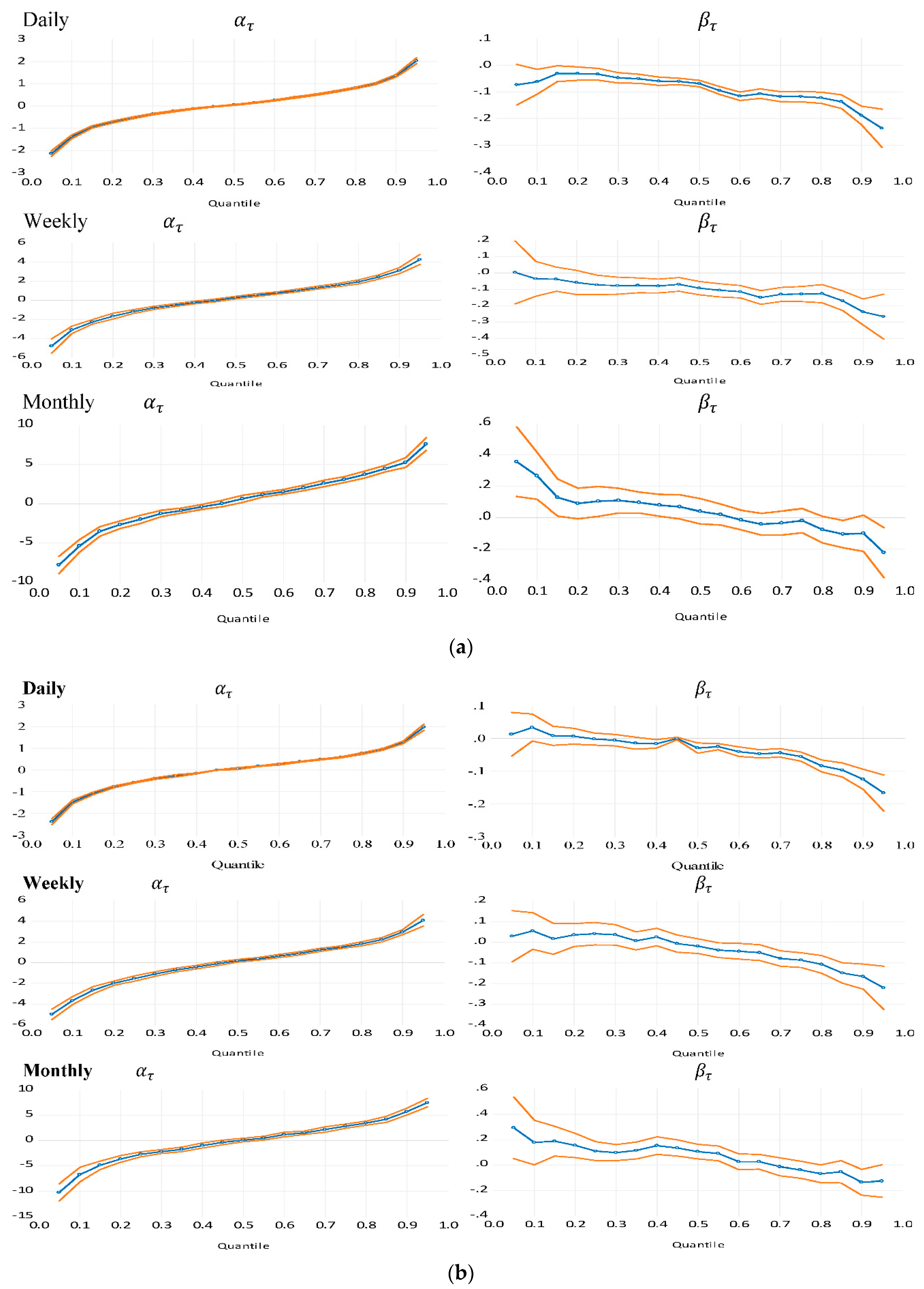
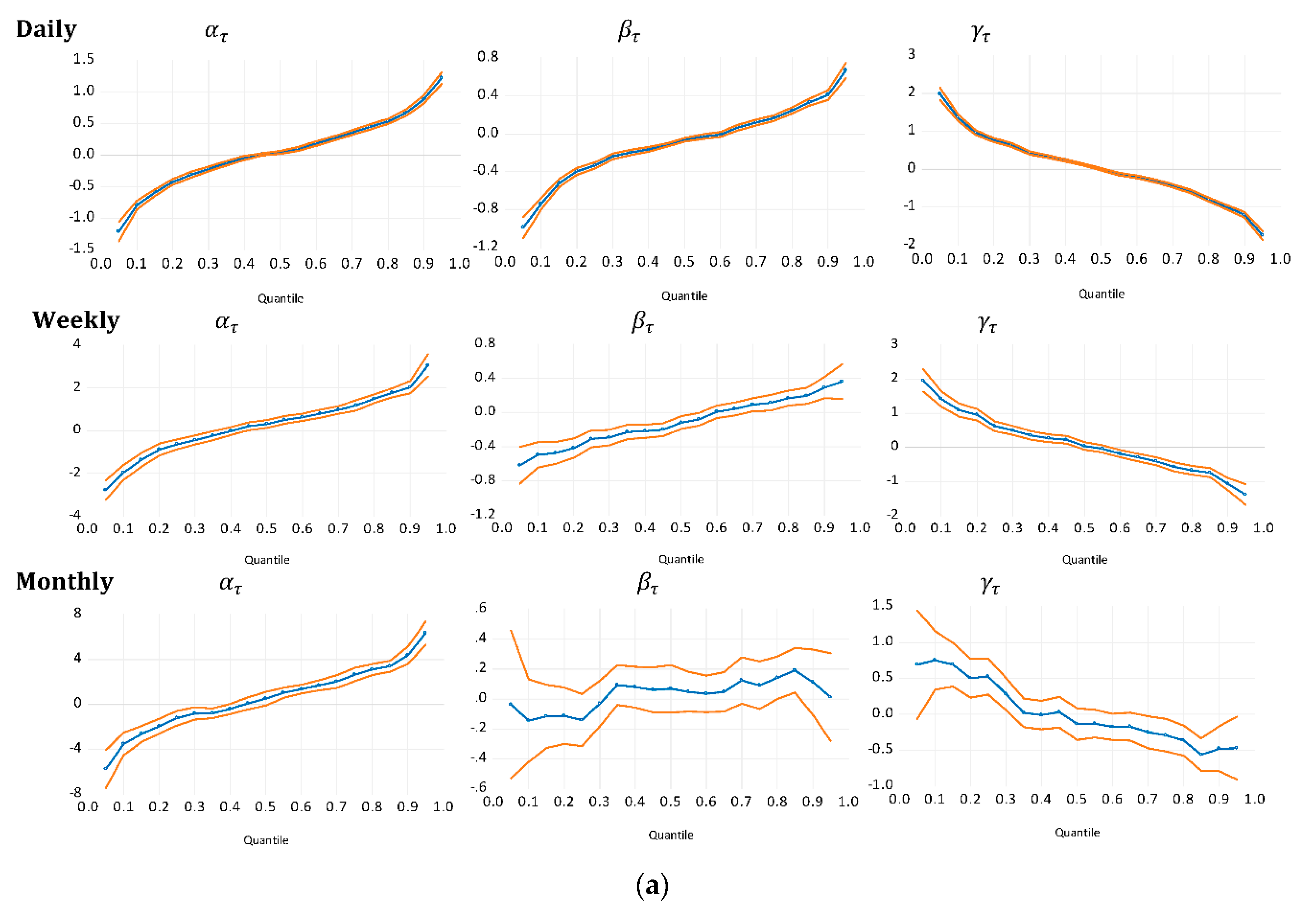
| 8 | For ease of interpretation of results, define 5th to 35th quantiles as lower quantiles, 40th to 70th quantiles as central or middle quantiles, and 75th to 95th quantiles as upper quantiles. |
| 9 | As Lewellen (2002) notes, momentum is not synonymous with positive autocorrelation. While momentum is a cross-sectional result where winning stocks beat losing stocks, autocorrelation is a time-series phenomenon where a stock’s or an index’s past and future returns are correlated. However, Lo and MacKinlay (1990) show that indeed, momentum may be caused by serial correlation of returns, lead-lag relations among stocks (cross-serial correlation), or cross-sectional dispersion in unconditional means. Lewellen (2002), for example, shows that negative autocorrelations tend to reduce momentum profits. |
| 10 | Anderson et al. (2013) intimate that daily return autocorrelation is attributable to market microstructure biases such as nonsynchronous trading effect and bid-ask bounce, partial price adjustment (PPA), and time-varying risk premia. However, Mech (1993) argues that weekly and monthly return autocorrelations are generally caused by changing investment opportunities, which are naturally low-frequency events. The strong daily return autocorrelation is also consistent with profit taking by technical analysts and day traders. |
| 11 | Since EREIT and MREIT are well diversified portfolios, their returns and dependence patterns reflect systematic risks caused by macroeconomic factors, as opposed to individual firm-specific or idiosyncratic risk. |
| 12 | See the studies by Holden and Subrahmanyam (2002); Mech (1993); Jennings et al. (1981) and Copeland (1976). |
| 13 | It should be noted that the primary source of income for MREITs is interest from the debt capital MREITs provide. While increase in interest rate (tightening monetary policy) may be indicative of healthy economic growth and inflation activity, which is good for MREITs, higher interest rates tend to decrease the value of mortgage-backed securities (MBS) and increase short-term borrowing costs for MREITs. Additionally, higher interest rates make the comparatively high MREITs’ dividend yields less appealing to income-seeking investors who may find the lower-risk, fixed income securities more attractive, thereby causing a decline in MREIT return autocorrelations. Therefore, positive market sentiments may result in declining MREIT returns. |
| 14 | |
| 15 | We also tested the effects on 90th and 97.5th percentiles of return on predictability of the conditional returns of EREITs and MREITs at different frequencies. The evidence remains qualitatively the same as shown in Table 4a,b. Results are available on request. |
| 16 | That is, 5th to 45th quantiles for the daily EREIT returns, 5th to 50th quantiles for the EREIT weekly returns and 5th to 25th quantiles for the monthly EREIT returns. The upper quantiles refer to 50th, 55th and 70th quantile and above for daily, weekly and monthly EREIT returns. Similar interpretations can be made from Table 4b. |
| 17 | Similar interpretations can be extended to the other quantiles. However, it should be noted the dummy estimates in Table 5a are mainly insignificant from the 40th and 65th quantiles and above for weekly and monthly returns. Similarly, the dummy coefficient estimates in Table 5b are insignificant across all quantiles for monthly returns. |
| 18 | The equation can be augmented with but the marginal impact of low and high volatility remain qualitatively the same with and without the lagged returns. |
| 19 | Other notable regulatory reforms were the formation of open-ended, REITs-devoted, mutual funds in 1985; the Tax Reform Act (TRA) of 1986, which abolished the favorable tax treatment of real estate limited partnerships, permitted internal advisement and management, and established vertical integration in the REITs industry; The inception of REITs’ initial public offering (IPO) in 1991; the IRS private letter ruling which paved the path for the creation of the umbrella partnership REITs (UPREIT) structure and the first UPREIT IPO in 1992; and the REIT Modernization Act (RMA) of 1999, which reduced required percentage of taxable income distributed to investors from 95% to 90% and permitted REITs to form wholly-owned, taxable REIT subsidiaries through which REITs could offer supplementary services to their tenants. |


| EREITs | MREITs | |||||
|---|---|---|---|---|---|---|
| Daily | Weekly | Monthly | Daily | Weekly | Monthly | |
| Mean | 0.014 | 0.070 | 0.303 | −0.031 | −0.153 | −0.601 |
| Maximum | 16.876 | 21.602 | 26.623 | 38.590 | 42.574 | 31.631 |
| Minimum | −21.532 | −29.862 | −38.434 | −38.693 | −47.464 | −79.44 |
| Std. Dev. | 1.765 | 3.450 | 5.062 | 2.016 | 4.135 | 6.6634 |
| Skewness | −0.547 *** | −0.744 *** | −1.462 *** | −0.415 *** | −2.214 *** | −3.339 *** |
| Kurtosis | 26.917 *** | 16.408 *** | 13.267 *** | 83.591 *** | 46.939 *** | 38.367 *** |
| Jarque−Bera | 134,137 *** | 8515 *** | 2754 *** | 1,519,959 *** | 91,257 *** | 31,306 *** |
| N | 5616 | 1123 | 580 | 5616 | 1123 | 580 |
| a | ||||||
| Q | Daily | Weekly | Monthly | |||
| AR(1) | 0.016 | −0.169 *** | 0.076 | −0.086 | 0.281 | 0.078 |
| 0.05 | −2.141 *** | −0.074 * | −4.792 *** | 0.003 | −7.792 *** | 0.356 *** |
| 0.10 | −1.391 *** | −0.062 ** | −3.099 *** | −0.036 | −5.376 *** | 0.265 *** |
| 0.15 | −0.950 *** | −0.032 ** | −2.261 *** | −0.039 | −3.510 *** | 0.128 ** |
| 0.20 | −0.723 *** | −0.032 ** | −1.665 *** | −0.059 | −2.641 *** | 0.090 * |
| 0.25 | −0.537 *** | −0.034 *** | −1.183 *** | −0.074 ** | −1.965 *** | 0.104 ** |
| 0.30 | −0.367 *** | −0.048 *** | −0.796 *** | −0.078 *** | −1.230 *** | 0.108 *** |
| 0.35 | −0.242 *** | −0.051 *** | −0.518 *** | −0.076 *** | −0.863 *** | 0.096 *** |
| 0.40 | −0.125 *** | −0.060 *** | −0.234 *** | −0.080 *** | −0.407 *** | 0.079 ** |
| 0.45 | −0.032 *** | −0.061 *** | −0.015 | −0.070 *** | 0.028 *** | 0.068 * |
| 0.50 | 0.044 *** | −0.069 *** | 0.283 *** | −0.093 *** | 0.624 *** | 0.040 *** |
| 0.55 | 0.139 *** | −0.095 *** | 0.534 *** | −0.106 *** | 1.161 *** | 0.020 |
| 0.60 | 0.250 *** | −0.117 *** | 0.757 *** | −0.115 *** | 1.523 *** | −0.015 |
| 0.65 | 0.379 *** | −0.107 *** | 1.023 *** | −0.150 *** | 2.018 *** | −0.041 |
| 0.70 | 0.500 *** | −0.118 *** | 1.324 *** | −0.131 *** | 2.591 *** | −0.034 |
| 0.75 | 0.650 *** | −0.118 *** | 1.597 *** | −0.129 *** | 3.093 *** | −0.019 |
| 0.80 | 0.813 *** | −0.123 *** | 1.931 *** | −0.127 *** | 3.726 *** | −0.076 * |
| 0.85 | 1.009 *** | −0.137 *** | 2.442 *** | −0.170 *** | 4.484 *** | −0.105 ** |
| 0.90 | 1.360 *** | −0.189 *** | 3.114 *** | −0.239 *** | 5.266 *** | −0.099 * |
| 0.95 | 2.030 *** | −0.237 *** | 4.267 *** | −0.267 *** | 7.620 | −0.223 *** |
| b | ||||||
| Daily | Weekly | Monthly | ||||
| AR(1) | −0.035 | −0.113 | −0.173 | −0.093 | −0.589 ** | 0.013 |
| 0.050 | −2.375 *** | 0.013 | −5.000 *** | 0.030 | −7.792 *** | 0.356 *** |
| 0.100 | −1.472 *** | 0.034 | −3.667 *** | 0.055 | −5.376 *** | 0.265 *** |
| 0.150 | −1.075 *** | 0.008 | −2.664 *** | 0.017 | −3.510 *** | 0.128 ** |
| 0.200 | −0.773 *** | 0.007 | −1.985 *** | 0.036 | −2.641 *** | 0.090 * |
| 0.250 | −0.571 *** | −0.002 | −1.532 *** | 0.042 | −1.965 *** | 0.104 ** |
| 0.300 | −0.392 *** | −0.005 | −1.091 *** | 0.036 | −1.230 *** | 0.108 *** |
| 0.350 | −0.269 *** | −0.015 | −0.703 *** | 0.007 | −0.863 ** | 0.096 *** |
| 0.400 | −0.158 *** | −0.017 ** | −0.425 *** | 0.025 | −0.407 | 0.079 ** |
| 0.450 | 0.000 | 0.001 *** | −0.098 | −0.006 | 0.028 *** | 0.068 *** |
| 0.500 | 0.069 *** | −0.029 *** | 0.187 *** | −0.018 | 0.624 *** | 0.040 |
| 0.550 | 0.174 *** | −0.025 *** | 0.384 ** | −0.038 ** | 1.161 *** | 0.020 |
| 0.600 | 0.270 *** | −0.040 *** | 0.648 ** | −0.043 ** | 1.523 *** | −0.015 |
| 0.650 | 0.380 *** | −0.047 *** | 0.910 ** | −0.050 ** | 2.018 *** | −0.041 |
| 0.700 | 0.486 *** | −0.044 *** | 1.249 *** | −0.079 *** | 2.591 *** | −0.034 |
| 0.750 | 0.585 *** | −0.055 *** | 1.494 *** | −0.086 *** | 3.093 *** | −0.019 |
| 0.800 | 0.757 *** | −0.084 *** | 1.829 *** | −0.107 *** | 3.726 *** | −0.076 * |
| 0.850 | 0.947 *** | −0.097 *** | 2.237 *** | −0.149 *** | 4.484 *** | −0.105 ** |
| 0.900 | 1.277 *** | −0.125 *** | 2.968 *** | −0.166 *** | 5.266 *** | −0.099 * |
| 0.950 | 1.974 *** | −0.167 *** | 4.107 *** | −0.221 *** | 7.620 *** | −0.223 |
| c | ||||||
| EREIT | MREIT | |||||
| Daily | Weekly | Monthly | Daily | Weekly | Monthly | |
| Null hypothesis | Chi-Sq. | Chi-Sq. | Chi-Sq. | Chi-Sq. | Chi-Sq. | Chi-Sq. |
| 22.180 *** | 7.427 ** | 19.105 *** | 27.035 *** | 15.984 *** | 15.189 *** | |
| 0.015 | 1.007 | 7.835 *** | 1.618 | 0.615 | 2.365 | |
| 22.175 *** | 6.411 ** | 10.194 *** | 25.461 *** | 15.361 *** | 12.493 *** | |
| 64.465 *** | 8.721 * | 20.085 *** | 48.096 *** | 33.114 *** | 29.486 *** | |
| All quantiles | 175.328 *** | 42.834 *** | 45.027 *** | 136.004 *** | 68.729 *** | 58.657 *** |
| a | |||||||||
| Daily | Weekly | Monthly | |||||||
| 0.05 | −1.216 *** | −0.990 *** | 1.989 *** | −2.783 *** | −0.618 *** | 1.953 *** | −5.768 *** | −0.037 | 0.688 * |
| 0.10 | −0.799 *** | −0.740 *** | 1.363 *** | −1.963 *** | −0.495 *** | 1.417 *** | −3.548 *** | −0.144 | 0.752 *** |
| 0.15 | −0.598 *** | −0.521 *** | 0.963 *** | −1.374 *** | −0.473 *** | 1.089 *** | −2.634 *** | −0.116 | 0.692 *** |
| 0.20 | −0.428 *** | −0.396 *** | 0.771 *** | −0.886 *** | −0.417 *** | 0.953 *** | −1.943 *** | −0.112 | 0.504 *** |
| 0.25 | −0.316 *** | −0.334 *** | 0.636 *** | −0.647 *** | −0.308 *** | 0.613 *** | −1.249 *** | −0.142 | 0.527 *** |
| 0.30 | −0.224 *** | −0.237 *** | 0.428 *** | −0.446 *** | −0.293 *** | 0.496 *** | −0.819 *** | −0.031 | 0.280 ** |
| 0.35 | −0.130 *** | −0.198 *** | 0.336 *** | −0.238 ** | −0.227 *** | 0.347 *** | −0.802 *** | 0.094 | 0.018 |
| 0.40 | −0.047 *** | −0.164 *** | 0.230 *** | −0.027 | −0.218 *** | 0.267 *** | −0.418 * | 0.079 | −0.012 |
| 0.45 | 0.009 | −0.119 *** | 0.121 *** | 0.199 ** | −0.201 *** | 0.220 *** | 0.073 | 0.061 | 0.028 |
| 0.50 | 0.041 *** | −0.064 *** | −0.007 | 0.311 *** | −0.118 *** | 0.036 | 0.496 *** | 0.069 | −0.136 |
| 0.55 | 0.094 *** | −0.031 *** | −0.132 *** | 0.499 *** | −0.080 ** | −0.045 | 1.027 *** | 0.048 | −0.131 |
| 0.60 | 0.181 *** | −0.008 | −0.205 *** | 0.621 *** | 0.008 | −0.188 *** | 1.346 *** | 0.034 | −0.176 * |
| 0.65 | 0.263 *** | 0.066 *** | −0.309 *** | 0.787 *** | 0.040 | −0.297 *** | 1.692 *** | 0.048 | −0.173 * |
| 0.70 | 0.353 *** | 0.119 *** | −0.443 *** | 0.961 *** | 0.091 ** | −0.411 *** | 2.029 *** | 0.124 | −0.250 ** |
| 0.75 | 0.444 *** | 0.166 *** | −0.592 *** | 1.181 *** | 0.114 ** | −0.570 *** | 2.650 *** | 0.092 | −0.293 ** |
| 0.80 | 0.531 *** | 0.247 *** | −0.806 *** | 1.486 *** | 0.169 *** | −0.675 *** | 3.107 *** | 0.142 * | −0.366 *** |
| 0.85 | 0.668 *** | 0.336 *** | −1.001 *** | 1.766 *** | 0.194 *** | −0.742 *** | 3.395 *** | 0.192 ** | −0.564 *** |
| 0.90 | 0.881 *** | 0.407 *** | −1.213 *** | 2.027 *** | 0.292 *** | −1.075 *** | 4.368 *** | 0.113 *** | −0.481 *** |
| 0.95 | 1.218 *** | 0.670 *** | −1.751 *** | 3.047 *** | 0.363 *** | −1.387 *** | 6.346 *** | 0.012 *** | −0.472 ** |
| b | |||||||||
| Daily | Weekly | Monthly | |||||||
| 0.05 | −1.574 *** | −0.619 *** | 1.525 *** | −3.384 *** | −0.639 *** | 1.933 *** | −5.768 *** | −0.037 | 0.688 * |
| 0.10 | −1.045 *** | −0.388 *** | 0.989 *** | −2.820 *** | −0.268 *** | 0.813 *** | −3.548 *** | −0.144 | 0.752 *** |
| 0.15 | −0.732 *** | −0.275 *** | 0.747 *** | −1.900 *** | −0.240 *** | 0.619 *** | −2.634 *** | −0.116 | 0.692 *** |
| 0.20 | −0.539 *** | −0.252 *** | 0.633 *** | −1.506 *** | −0.196 *** | 0.477 *** | −1.943 *** | −0.112 | 0.504 *** |
| 0.25 | −0.381 *** | −0.209 *** | 0.488 *** | −1.094 *** | −0.183 *** | 0.417 *** | −1.249 *** | −0.142 | 0.527 *** |
| 0.30 | −0.281 *** | −0.152 *** | 0.342 *** | −0.784 *** | −0.152 *** | 0.311 *** | −0.819 *** | −0.031 | 0.280 ** |
| 0.35 | −0.164 *** | −0.133 *** | 0.252 *** | −0.499 *** | −0.109 *** | 0.237 *** | −0.802 *** | 0.094 | 0.018 |
| 0.40 | −0.117 *** | −0.075 *** | 0.126 *** | −0.258 ** | −0.090 ** | 0.179 *** | −0.418 * | 0.079 | −0.012 |
| 0.45 | 0.000 | −0.028 *** | 0.028 ** | 0.081 | −0.098 *** | 0.197 *** | 0.073 *** | 0.061 | 0.028 |
| 0.50 | 0.058 ** | −0.020 * | −0.022 | 0.275 *** | −0.078 ** | 0.110 ** | 0.496 *** | 0.069 | −0.136 |
| 0.55 | 0.156 *** | 0.006 | −0.063 *** | 0.371 *** | −0.029 | −0.024 | 1.027 *** | 0.048 | −0.131 |
| 0.60 | 0.189 *** | 0.051 *** | −0.195 *** | 0.574 *** | −0.002 | −0.063 | 1.346 *** | 0.034 | −0.176 *** |
| 0.65 | 0.290 *** | 0.085 *** | −0.271 *** | 0.845 *** | −0.012 | −0.093 * | 1.692 *** | 0.048 | −0.173 * |
| 0.70 | 0.347 *** | 0.134 *** | −0.403 *** | 1.016 *** | 0.039 | −0.224 *** | 2.029 *** | 0.124 | −0.250 ** |
| 0.75 | 0.404 *** | 0.200 *** | −0.594 *** | 1.268 *** | 0.038 | −0.319 *** | 2.650 *** | 0.092 | −0.293 ** |
| 0.80 | 0.478 *** | 0.323 *** | −0.829 *** | 1.497 *** | 0.107 *** | −0.383 *** | 3.107 *** | 0.142 * | −0.366 *** |
| 0.85 | 0.556 *** | 0.473 *** | −1.148 *** | 1.686 *** | 0.158 *** | −0.594 *** | 3.395 *** | 0.192 ** | −0.564 *** |
| 0.90 | 0.722 *** | 0.591 *** | −1.475 *** | 1.834 *** | 0.372 *** | −1.282 *** | 4.368 *** | 0.113 | −0.481 *** |
| 0.95 | 1.092 *** | 0.810 *** | −1.779 *** | 2.633 *** | 0.571 *** | −1.464 *** | 6.346 *** | 0.012 | −0.472 ** |
| a | |||||||||
| Daily | Weekly | Monthly | |||||||
| 0.05 | −1.945 *** | −0.013 | −0.908 *** | −4.176 *** | 0.147 * | −1.131 *** | −7.086 *** | 0.165 | −0.710 *** |
| 0.10 | −1.253 *** | −0.009 | −0.692 *** | −2.912 *** | 0.142 *** | −0.732 *** | −4.665 *** | 0.140 * | −0.439 *** |
| 0.15 | −0.897 *** | −0.018 | −0.449 *** | −2.243 *** | 0.076 ** | −0.628 *** | −3.259 *** | 0.076 | −0.539 *** |
| 0.20 | −0.677 *** | −0.009 | −0.370 *** | −1.585 *** | 0.027 | −0.501 *** | −2.551 *** | 0.110 ** | −0.453 *** |
| 0.25 | −0.507 *** | −0.012 | −0.294 *** | −1.128 *** | −0.044 | −0.350 *** | −1.918 *** | 0.112 ** | −0.282 *** |
| 0.30 | −0.352 *** | −0.023 ** | −0.209 *** | −0.746 *** | −0.034 | −0.268 *** | −1.227 *** | 0.103 ** | 0.007 |
| 0.35 | −0.231 *** | −0.034 *** | −0.158 *** | −0.475 *** | −0.073 *** | −0.203 *** | −0.885 *** | 0.075 ** | 0.022 |
| 0.40 | −0.123 *** | −0.048 *** | −0.108 *** | −0.219 *** | −0.074 *** | −0.135 *** | −0.412 ** | 0.071 * | 0.010 |
| 0.45 | −0.029 *** | −0.058 *** | −0.053 *** | 0.028 | −0.099 *** | −0.099 *** | 0.015 | 0.074 * | −0.011 |
| 0.50 | 0.042 *** | −0.069 *** | 0.058 *** | 0.286 *** | −0.109 *** | −0.101 *** | 0.701 *** | 0.007 | 0.063 |
| 0.55 | 0.132 *** | −0.091 *** | 0.081 *** | 0.530 *** | −0.095 *** | 0.091 *** | 1.119 *** | −0.010 | 0.069 |
| 0.60 | 0.234 *** | −0.097 *** | 0.137 *** | 0.756 *** | −0.078 *** | 0.168 *** | 1.512 *** | −0.023 | 0.039 |
| 0.65 | 0.359 *** | −0.096 *** | 0.170 *** | 0.968 *** | −0.086 *** | 0.178 *** | 1.931 *** | −0.036 | 0.064 |
| 0.70 | 0.477 *** | −0.109 *** | 0.252 *** | 1.268 *** | −0.128 *** | 0.326 *** | 2.496 *** | −0.016 | 0.192 *** |
| 0.75 | 0.622 *** | −0.116 *** | 0.376 *** | 1.544 *** | −0.147 *** | 0.356 *** | 3.036 *** | −0.005 | 0.182 *** |
| 0.80 | 0.786 *** | −0.116 *** | 0.456 *** | 1.888 *** | −0.135 *** | 0.357 *** | 3.615 *** | −0.026 | 0.150 ** |
| 0.85 | 0.951 *** | −0.105 *** | 0.579 *** | 2.357 *** | −0.167 *** | 0.412 *** | 4.344 *** | −0.082 * | 0.196 *** |
| 0.90 | 1.260 *** | −0.142 *** | 0.653 *** | 2.837 *** | −0.203 *** | 0.591 *** | 5.171 *** | −0.082 | 0.256 *** |
| 0.95 | 1.762 *** | −0.163 *** | 0.942 *** | 3.811 *** | −0.301 *** | 0.897 *** | 6.768 *** | −0.059 | 0.479 *** |
| b | |||||||||
| Daily | Weekly | Monthly | |||||||
| 0.05 | −2.144 *** | 0.178 *** | −0.564 *** | −4.715 *** | 0.179 *** | −1.314 *** | −9.885 *** | 0.263 | −0.238 *** |
| 0.10 | −1.384 *** | 0.107 *** | −0.452 *** | −3.479 *** | 0.123 ** | −0.621 *** | −6.516 *** | 0.159 | −0.241 *** |
| 0.15 | −1.017 *** | 0.070 *** | −0.304 *** | −2.456 *** | 0.016 | −0.332 *** | −4.812 *** | 0.116 | −0.252 ** |
| 0.20 | −0.743 *** | 0.058 *** | −0.280 *** | −1.896 *** | 0.014 | −0.228 *** | −3.530 *** | 0.095 | −0.271 *** |
| 0.25 | −0.546 *** | 0.035 *** | −0.223 *** | −1.435 *** | 0.006 | −0.178 *** | −2.732 *** | 0.109 ** | −0.154 ** |
| 0.30 | −0.384 *** | 0.024 *** | −0.150 *** | −1.051 *** | 0.000 | −0.105 *** | −2.174 *** | 0.117 *** | 0.022 |
| 0.35 | −0.242 *** | −0.010 | −0.107 *** | −0.680 *** | −0.004 | −0.123 *** | −1.701 *** | 0.127 *** | 0.080 |
| 0.40 | −0.156 *** | −0.010 | −0.050 *** | −0.417 *** | 0.009 | −0.095 *** | −1.068 *** | 0.141 *** | 0.088 |
| 0.45 | 0.000 | 0.000 | −0.028 *** | −0.057 | 0.000 | −0.095 *** | −0.436 * | 0.152 *** | 0.175 *** |
| 0.50 | 0.065 *** | −0.035 *** | 0.025 *** | 0.187 *** | −0.007 | −0.093 *** | 0.069 | 0.108 *** | 0.222 *** |
| 0.55 | 0.172 *** | −0.021 *** | 0.043 *** | 0.383 *** | −0.038 ** | 0.008 | 0.404 ** | 0.100 *** | 0.277 *** |
| 0.60 | 0.260 *** | −0.057 *** | 0.122 *** | 0.626 *** | −0.036 * | 0.021 | 0.873 *** | 0.115 *** | 0.276 *** |
| 0.65 | 0.369 *** | −0.055 *** | 0.170 *** | 0.901 *** | −0.054 *** | 0.033 | 1.459 *** | 0.074 * | 0.276 *** |
| 0.70 | 0.471 *** | −0.062 *** | 0.319 *** | 1.243 *** | −0.074 *** | 0.032 | 1.795 *** | 0.085 ** | 0.283 *** |
| 0.75 | 0.565 *** | −0.052 *** | 0.433 *** | 1.487 *** | −0.104 *** | 0.171 *** | 2.753 *** | 0.055 *** | 0.240 *** |
| 0.80 | 0.716 *** | −0.075 *** | 0.539 *** | 1.772 *** | −0.089 *** | 0.181 *** | 3.355 *** | 0.057 *** | 0.235 *** |
| 0.85 | 0.884 *** | −0.085 *** | 0.690 *** | 2.200 *** | −0.141 *** | 0.735 *** | 4.010 *** | 0.063 *** | 0.233 *** |
| 0.90 | 1.169 *** | −0.101 *** | 0.844 *** | 2.858 *** | −0.145 *** | 0.743 *** | 5.288 *** | 0.070 *** | 0.324 *** |
| 0.95 | 1.711 *** | −0.099 *** | 1.042 *** | 3.643 *** | −0.209 *** | 0.789 *** | 6.982 *** | 0.026 *** | 0.206 * |
| a | |||||||||
| Daily | Weekly | Monthly | |||||||
| 0.05 | −2.176 *** | 0.057 | −0.274 *** | −4.888 *** | −0.027 | 0.342 * | −7.275 *** | 0.234 | 0.277 |
| 0.10 | −1.386 *** | 0.050 | −0.273 *** | −3.088 *** | −0.076 | 0.267 *** | −4.763 *** | 0.044 | 0.406 *** |
| 0.15 | −0.957 *** | 0.036 | −0.232 *** | −2.289 *** | −0.064 | 0.194 ** | −3.332 *** | −0.007 | 0.480 *** |
| 0.20 | −0.732 *** | 0.039 ** | −0.227 *** | −1.620 *** | −0.103 ** | 0.241 *** | −2.495 *** | −0.022 | 0.421 *** |
| 0.25 | −0.532 *** | 0.038 ** | −0.245 *** | −1.204 *** | −0.089 ** | 0.202 *** | −1.936 *** | −0.037 | 0.378 *** |
| 0.30 | −0.377 *** | 0.023 *** | −0.240 *** | −0.779 *** | −0.087 *** | 0.129 ** | −1.246 *** | −0.013 | 0.310 *** |
| 0.35 | −0.253 *** | 0.009 | −0.221 *** | −0.523 *** | −0.087 *** | 0.144 *** | −0.819 *** | 0.010 | 0.217 *** |
| 0.40 | −0.132 *** | −0.006 *** | −0.194 *** | −0.239 *** | −0.091 *** | 0.022 | −0.317 * | 0.009 | 0.165 ** |
| 0.45 | −0.018 | −0.013 | −0.192 *** | −0.003 | −0.083 *** | 0.040 | 0.136 | −0.020 | 0.148 *** |
| 0.50 | 0.026 *** | −0.016 ** | −0.191 *** | 0.286 *** | −0.109 *** | 0.101 ** | 0.776 *** | −0.051 | 0.191 ** |
| 0.55 | 0.131 *** | −0.033 *** | −0.181 *** | 0.538 *** | −0.107 *** | 0.021 | 1.213 *** | −0.053 | 0.221 *** |
| 0.60 | 0.246 *** | −0.047 *** | −0.176 *** | 0.759 *** | −0.117 *** | 0.058 | 1.587 *** | −0.070 *** | 0.146 ** |
| 0.65 | 0.376 *** | −0.052 *** | −0.177 *** | 1.023 *** | −0.150 *** | −0.004 | 1.922 *** | −0.080 *** | 0.108 |
| 0.70 | 0.503 *** | −0.047 *** | −0.198 *** | 1.325 *** | −0.142 *** | 0.011 | 2.540 *** | −0.059 | 0.039 |
| 0.75 | 0.646 *** | −0.053 *** | −0.193 *** | 1.597 *** | −0.129 *** | 0.020 | 3.169 *** | −0.108 ** | 0.115 |
| 0.80 | 0.819 *** | −0.046 *** | −0.210 *** | 1.966 *** | −0.140 *** | 0.044 | 3.748 *** | −0.131 ** | 0.163 * |
| 0.85 | 1.013 *** | −0.049 *** | −0.227 *** | 2.442 *** | −0.170 *** | −0.167 *** | 4.492 *** | −0.122 ** | 0.017 |
| 0.90 | 1.338 *** | −0.092 *** | −0.212 *** | 3.090 *** | −0.232 *** | −0.044 | 5.233 *** | −0.093 | −0.031 |
| 0.95 | 2.016 *** | −0.165 *** | −0.227 *** | 4.223 *** | −0.287 *** | 0.119 | 7.643 *** | −0.228 ** | 0.004 |
| b | |||||||||
| Daily | Weekly | Monthly | |||||||
| 0.05 | −2.362 *** | 0.079 *** | −0.174 ** | −4.984 *** | 0.021 | 0.165 | −10.177 *** | 0.293 * | −0.004 |
| 0.10 | −1.476 *** | 0.088 *** | −0.218 *** | −3.686 *** | 0.014 | 0.181 * | −6.806 *** | 0.169 | 0.146 |
| 0.15 | −1.088 *** | 0.072 *** | −0.164 *** | −2.664 *** | 0.017 | 0.172 * | −4.898 *** | 0.187 ** | 0.093 |
| 0.20 | −0.774 *** | 0.059 *** | −0.164 *** | −1.955 *** | −0.005 | 0.153 *** | −3.679 *** | 0.155 *** | 0.133 |
| 0.25 | −0.561 *** | 0.046 *** | −0.161 *** | −1.536 *** | −0.046 | 0.169 *** | −2.723 *** | 0.082 * | 0.093 |
| 0.30 | −0.398 *** | 0.038 *** | −0.160 *** | −1.117 *** | −0.025 | 0.122 * | −2.178 *** | 0.095 ** | 0.030 |
| 0.35 | −0.272 *** | 0.032 *** | −0.162 *** | −0.698 *** | −0.033 | 0.108 * | −1.763 *** | 0.091 ** | 0.027 |
| 0.40 | −0.164 *** | 0.009 | −0.142 *** | −0.451 *** | −0.042 * | 0.125 *** | −0.989 *** | 0.142 *** | 0.016 |
| 0.45 | 0.000 | 0.000 | −0.140 *** | −0.071 | −0.064 *** | 0.158 *** | −0.343 | 0.111 *** | 0.080 |
| 0.50 | 0.074 * | 0.011 | −0.154 *** | 0.160 ** | −0.069 *** | 0.145 *** | 0.083 | 0.102 *** | 0.107 |
| 0.55 | 0.173 *** | −0.003 | −0.146 *** | 0.380 *** | −0.070 *** | 0.101 *** | 0.463 ** | 0.091 ** | 0.037 |
| 0.60 | 0.285 *** | −0.005 | −0.149 *** | 0.668 *** | −0.070 *** | 0.077 | 1.151 *** | 0.010 | 0.083 |
| 0.65 | 0.377 *** | −0.017 ** | −0.141 *** | 0.911 *** | −0.090 *** | 0.126 *** | 1.525 *** | 0.025 | 0.062 |
| 0.70 | 0.488 *** | −0.036 *** | −0.126 *** | 1.226 *** | −0.089 *** | 0.128 *** | 2.192 *** | −0.047 | 0.077 |
| 0.75 | 0.588 *** | −0.041 *** | −0.126 *** | 1.490 *** | −0.105 *** | 0.130 *** | 2.872 *** | −0.075 * | 0.072 |
| 0.80 | 0.758 *** | −0.047 *** | −0.134 *** | 1.796 *** | −0.138 *** | 0.140 ** | 3.411 *** | −0.071 * | 0.090 |
| 0.85 | 0.959 *** | −0.053 *** | −0.155 *** | 2.237 *** | −0.149 *** | 0.079 | 4.218 *** | −0.084 | 0.135 |
| 0.90 | 1.287 *** | −0.061 *** | −0.190 *** | 2.959 *** | −0.166 *** | 0.049 | 5.792 *** | −0.147 | 0.088 |
| 0.95 | 1.961 *** | −0.081 *** | −0.255 *** | 4.007 *** | −0.223 *** | 0.017 | 7.334 *** | −0.128 * | 0.096 |
| a | ||||||
| Daily | Weekly | Monthly | ||||
| 0.05 | 0.052 | −0.205 *** | 0.228 | −0.042 | 0.381 ** | 0.355 ** |
| 0.10 | 0.039 | −0.260 *** | 0.107 | −0.086 | 0.238 * | 0.266 *** |
| 0.15 | 0.033 | −0.231 *** | 0.045 | −0.112 ** | 0.091 | 0.196 *** |
| 0.20 | 0.032 * | −0.227 *** | 0.050 | −0.142 *** | 0.025 | 0.165 *** |
| 0.25 | 0.033 ** | −0.234 *** | −0.017 | −0.163 *** | 0.018 | 0.139 ** |
| 0.30 | 0.024 * | −0.232 *** | −0.008 | −0.158 *** | 0.102 | 0.110 ** |
| 0.35 | 0.005 | −0.244 *** | −0.037 | −0.158 *** | 0.103 * | 0.095 ** |
| 0.40 | −0.008 * | −0.251 *** | −0.028 | −0.205 *** | 0.095 * | 0.068 |
| 0.45 | −0.015 | −0.245 *** | −0.044 | −0.219 *** | 0.100 | 0.040 |
| 0.50 | −0.017 ** | −0.243 *** | −0.058 | −0.214 *** | 0.119 * | 0.022 |
| 0.55 | −0.036 *** | −0.239 *** | −0.081 ** | −0.244 *** | 0.022 | 0.019 |
| 0.60 | −0.056 *** | −0.233 *** | −0.078 ** | −0.256 *** | −0.012 | −0.015 |
| 0.65 | −0.055 *** | −0.229 *** | −0.086 ** | −0.265 *** | 0.018 | −0.042 |
| 0.70 | −0.054 *** | −0.237 *** | −0.106 *** | −0.280 *** | −0.006 | −0.038 |
| 0.75 | −0.064 *** | −0.246 *** | −0.113 *** | −0.293 *** | 0.015 | −0.079 |
| 0.80 | −0.063 *** | −0.257 *** | −0.102 * | −0.310 *** | 0.043 | −0.134 |
| 0.85 | −0.057 *** | −0.276 *** | −0.116 ** | −0.334 *** | −0.039 | −0.130 ** |
| 0.90 | −0.102 *** | −0.290 *** | −0.148 ** | −0.328 *** | −0.067 | −0.122 * |
| 0.95 | −0.193 *** | −0.334 *** | −0.185 | −0.296 *** | −0.268 ** | −0.219 ** |
| b | ||||||
| Daily | Weekly | Monthly | ||||
| 0.05 | 0.208 *** | −0.033 | 0.342 ** | 0.030 | 0.675 *** | 0.060 |
| 0.10 | 0.158 *** | −0.050 * | 0.145 | 0.014 | 0.509 *** | −0.010 |
| 0.15 | 0.120 *** | −0.034 * | 0.094 | 0.014 | 0.324 *** | −0.018 |
| 0.20 | 0.100 *** | −0.041 *** | 0.012 | 0.036 | 0.327 *** | 0.024 |
| 0.25 | 0.073 *** | −0.043 *** | −0.042 | 0.050 | 0.300 *** | 0.030 |
| 0.30 | 0.065 *** | −0.071 *** | −0.036 | 0.062 * | 0.308 *** | −0.007 |
| 0.35 | 0.073 *** | −0.072 *** | −0.025 | 0.060 * | 0.298 *** | −0.032 |
| 0.40 | 0.041 *** | −0.069 *** | −0.002 | 0.029 | 0.275 *** | −0.056 |
| 0.45 | 0.000 | −0.076 *** | −0.073 | 0.015 | 0.243 *** | −0.035 |
| 0.50 | 0.037 *** | −0.071 *** | −0.057 | 0.000 | 0.194 *** | −0.006 |
| 0.55 | 0.010 | −0.074 *** | −0.050 | −0.032 | 0.140 * | −0.072 * |
| 0.60 | 0.027 | −0.089 *** | −0.029 | −0.044 * | 0.131 * | −0.077 * |
| 0.65 | 0.005 | −0.099 *** | −0.011 | −0.093 *** | 0.084 | −0.055 |
| 0.70 | −0.016 | −0.111 *** | −0.031 | −0.100 *** | 0.119 * | −0.072 * |
| 0.75 | −0.020 * | −0.115 *** | −0.017 | −0.132 *** | 0.069 | −0.152 *** |
| 0.80 | −0.046 *** | −0.112 *** | 0.008 | −0.158 *** | 0.067 | −0.161 *** |
| 0.85 | −0.075 *** | −0.132 *** | 0.013 | −0.217 *** | 0.037 | −0.167 *** |
| 0.90 | −0.121 *** | −0.126 *** | −0.002 | −0.248 *** | 0.012 | −0.149 * |
| 0.95 | −0.248 *** | −0.098 *** | −0.047 | −0.222 *** | 0.026 | −0.132 * |
| EREITs | MREITs | |||||
|---|---|---|---|---|---|---|
| 0.05 | −7.810 *** | 0.354 | 0.357 *** | −10.276 *** | 0.276 | 0.152 |
| 0.10 | −4.711 *** | 0.409 * | 0.147 | −6.840 *** | 0.606 ** | 0.195 * |
| 0.15 | −3.499 *** | 0.430 ** | 0.048 | −4.897 *** | 0.212 | 0.244 *** |
| 0.20 | −2.586 *** | 0.313 ** | 0.011 | −3.606 *** | 0.165 | 0.210 *** |
| 0.25 | −2.041 *** | 0.295 ** | −0.005 | −2.713 *** | 0.212 * | 0.111 ** |
| 0.30 | −1.323 *** | 0.278 ** | 0.001 | −2.155 *** | 0.233 * | 0.113 *** |
| 0.35 | −0.823 *** | 0.227 ** | 0.022 | −1.660 *** | 0.295 ** | 0.120 *** |
| 0.40 | −0.338 * | 0.258 ** | 0.037 | −1.080 *** | 0.273 ** | 0.147 *** |
| 0.45 | 0.002 | 0.245 ** | 0.014 | −0.369 * | 0.247 ** | 0.105 *** |
| 0.50 | 0.692 *** | 0.217 * | −0.037 | 0.008 | 0.239 ** | 0.085 ** |
| 0.55 | 1.146 *** | 0.263 ** | −0.067 | 0.477 | 0.265 ** | 0.089 ** |
| 0.60 | 1.598 *** | 0.131 | −0.103 *** | 1.173 *** | 0.324 *** | −0.001 |
| 0.65 | 1.939 *** | 0.175 | −0.092 ** | 1.535 *** | 0.308 *** | −0.055 |
| 0.70 | 2.549 *** | 0.103 | −0.095 ** | 2.205 *** | 0.279 ** | −0.068 |
| 0.75 | 3.119 *** | 0.085 | −0.152 *** | 2.799 *** | 0.319 *** | −0.075 * |
| 0.80 | 3.759 *** | 0.122 | −0.150 *** | 3.302 *** | 0.293 ** | −0.088 * |
| 0.85 | 4.412 *** | 0.068 | −0.127 ** | 4.423 *** | 0.442 ** | −0.130 ** |
| 0.90 | 5.104 *** | 0.014 | −0.128 * | 5.759 *** | 0.380 ** | −0.148 ** |
| 0.95 | 7.451 *** | 0.058 | −0.216 ** | 7.107 *** | 0.248 | −0.131 * |
Publisher’s Note: MDPI stays neutral with regard to jurisdictional claims in published maps and institutional affiliations. |
© 2020 by the authors. Licensee MDPI, Basel, Switzerland. This article is an open access article distributed under the terms and conditions of the Creative Commons Attribution (CC BY) license (http://creativecommons.org/licenses/by/4.0/).
Share and Cite
Ngene, G.M.; Manohar, C.A.; Julio, I.F. Overreaction in the REITs Market: New Evidence from Quantile Autoregression Approach. J. Risk Financial Manag. 2020, 13, 282. https://doi.org/10.3390/jrfm13110282
Ngene GM, Manohar CA, Julio IF. Overreaction in the REITs Market: New Evidence from Quantile Autoregression Approach. Journal of Risk and Financial Management. 2020; 13(11):282. https://doi.org/10.3390/jrfm13110282
Chicago/Turabian StyleNgene, Geoffrey M., Catherine Anitha Manohar, and Ivan F. Julio. 2020. "Overreaction in the REITs Market: New Evidence from Quantile Autoregression Approach" Journal of Risk and Financial Management 13, no. 11: 282. https://doi.org/10.3390/jrfm13110282
APA StyleNgene, G. M., Manohar, C. A., & Julio, I. F. (2020). Overreaction in the REITs Market: New Evidence from Quantile Autoregression Approach. Journal of Risk and Financial Management, 13(11), 282. https://doi.org/10.3390/jrfm13110282