1. Introduction
Gervais et al. (
2001) examined the relationship between extreme trading activity and the evolution of stock prices. They found that unusually high or low trading volumes, measured over a day or a week, are often followed by relatively high or low stock returns. Inspired by this study, many other researchers have examined the impacts of unusual trading volume, such as changes in visibility and short-selling constraints. Most studies have focused on stock markets in developed countries, especially in the United States. However, there has been little characterization of these trends in the Chinese market. The trading volume in China is influenced by international financial development and the integration of China within world financial markets. Increasing connections across world financial markets indicate the integration of stock market risks, which play a central role in international portfolio diversification (
Marfatia 2017). Marfatia found that risks in the U.S. and European markets comove strongly. However, risks in individual stock markets are more integrated with the region in which the country belongs, and less so with the U.S. or other regions.
Ji et al. (
2018) analyzed information spillovers of leading real estate markets across the world. The results showed a pairwise transfer entropy between countries such as the US, France and New Zealand.
Chatziantoniou et al. (
2020) investigated stock market sectoral connectedness and found that this varies with time. This study explores the relationship between unusual trading volume and earnings surprises for individual stocks in China.
First, we empirically examined whether extreme trading activities play an informational role in predicting earnings surprises in China’s market. Unusually high and low trading volume might indicate significant, unexpected earnings. In contrast to what has been observed in the United States, stocks with unusually high trading volume may experience lower returns, and those with unusually low trading volume may experience higher returns close to the earnings announcement date in China. This is because the high-volume return premium, a significant component of the United States stock market, does not exist in China, which is a difference in the nature of the market. Stocks that are subject to divergent opinions and short-selling constraints may be biased upwards and thus experience negative return near an earnings announcement date, and vice versa. However, consistent with the situation in the United States, stocks with unusually low trading volume prior to earnings announcements may have relatively lower unexpected earnings in terms of standard unexpected earnings (SUE). SUE are closely related to firm fundamentals, which can be considered as cash flow. Unusually low trading volume indicates low divergence of opinion and a consensus that there are relatively worse fundamentals because, under short-selling constraints, agents who are informed of bad news incline to avoid trading. Our findings suggest that the drivers and the mechanisms of earnings surprises in terms of cash flow and market expectations are different in China.
The ability of an unusually high trading volume to predict higher return is similar in the stock markets of some developed countries, especially the United States.
Gervais et al. (
2001) used data from 1963 to 1996 to examine the high-volume premium in the United States market.
Chen et al. (
2001) examined the markets of nine developed regions and found a positive correlation between trading volume and stock price change from 1973 to 2000.
Mayshar (
1983) postulated that holders of a specific stock are more optimistic about its prospects; an unusually high volume would suddenly increase the visibility of the stock, leading to higher demand from and price expectations of its holder.
Kaniel et al. (
2012) explained that increased visibility of a stock also increases its investor base, with a concomitant reduction in the cost of capital. In China, however, an unusually high trading volume signals a lower return, and unusually low trading volume predicts a higher return. This opposite effect might suggest another explanation.
Banerjee and Kremer (
2010) found that unusually high volume indicates a greater divergence of opinion about stock prospects.
Miller (
1977) hypothesized that prices of stocks without short-selling are biased upwards if there is high divergence of opinion.
Berkman et al. (
2009) found that, if earnings announcements reduce differences of opinion and overvaluation, stocks with high difference of opinion and stricter short-selling constraints often experience a decline in price around the earnings announcement date. By the same logic, it could be deduced that, if views on a stock with lower difference of opinion before the earnings announcement become more divergent after the announcement, the stock tends to have a higher excess return, relative to the market close to the earnings announcement date.
For unusually low trading volume,
Diamond and Verrecchia (
1987) argue that prohibiting traders from short-selling increases the time needed for the market price to adjust to private information, especially bad news. Thus, under short-selling constraints, the instantaneous price of a stock might not reflect the market expectation of all agents. If some agents receive bad news, they may be inclined not to trade, thus decreasing trading volume.
Akbas (
2016) invoked this argument and provided evidence from the United States market that an unusually low trading volume signals weak firm fundamentals. The negative relationship between an unusually low trading volume and firm fundamentals becomes more significant for firms with severer short-selling constraints.
Earnings announcements are scheduled regularly every quarter. The management of the firm tries to convey relevant information about expected cash flows to the market through this process. In addition to any information about current earnings, quarterly announcements also provide substantial details that could help investors acquire better understanding of the firm’s prospects. Thus, this information could be used to examine whether any signal received prior to the announcement date contains information about firm fundamentals.
The primary contribution of this study is to examine if an unusual trading volume predicts earnings surprises in China’s market. We present evidence that an unusually low trading volume predicts lower cash flow and a higher return, and an unusually high trading volume predicts a lower return, which is quite different from the relationship observed in markets in the United States and most developed countries. Additionally, we improve the existing methodology by using a fixed effect regression to analyze panel data, focusing on each individual stock rather than portfolios, making the results more reliable.
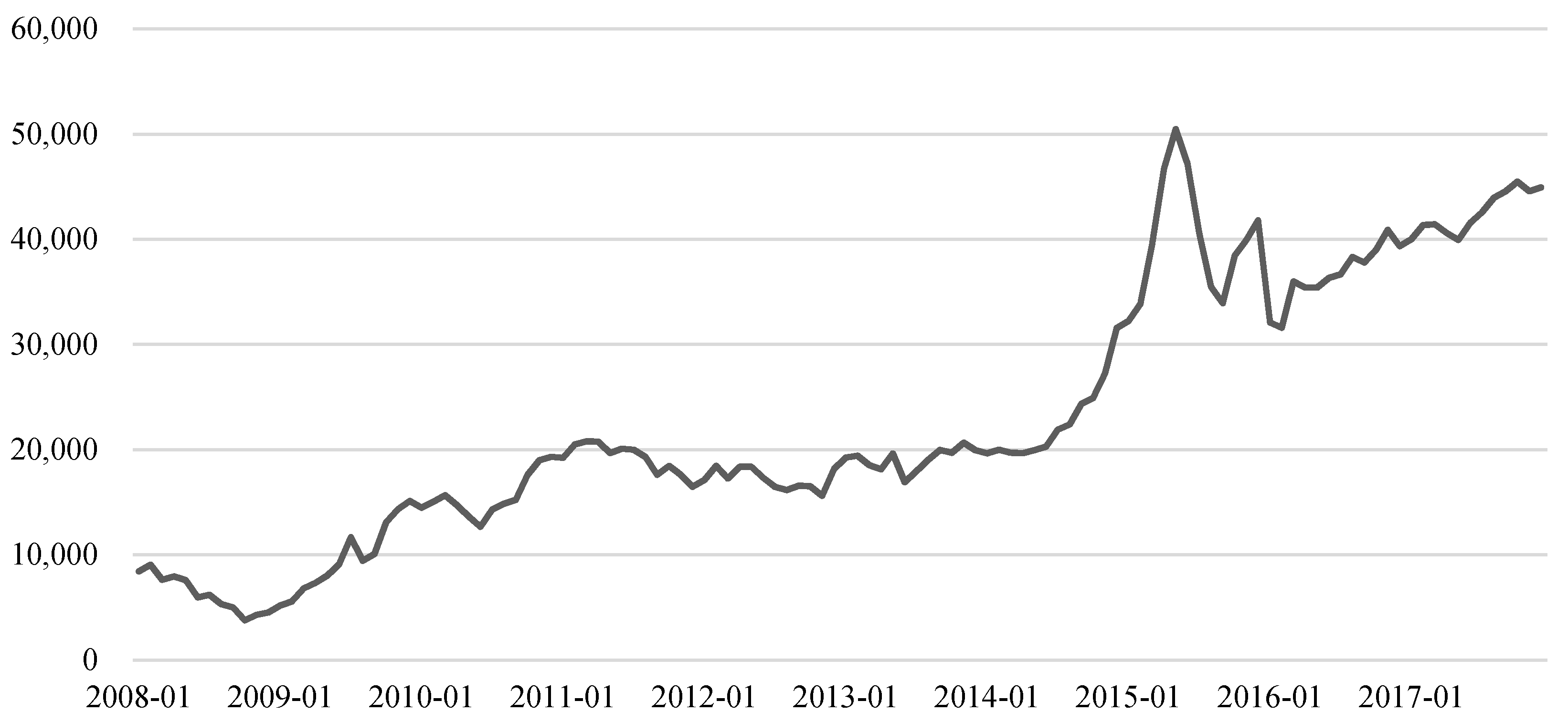
It is important to study the Chinese market for several reasons. First, the Chinese equity market has expanded rapidly recently. From January 2000 to December 2017, the number of stocks increased from 1206 to 3567, and the total market capitalization has exceeded 8.7 trillion dollars. Since China’s stock market has become an important part of the global economy and is incorporated into the global capitalization market through the Qualified Foreign Institutional Investor (QFII) system, insights into the Chinese stock market may help global investors make better decisions.
Second, China’s stock market is quite different from that of the United States. There are strict short-selling constraints for the A-share market. Firms issue two types of shares: A-shares and B-shares. Class A shares are priced and traded in RMB and among Chinese citizens, while class B shares are traded in foreign currencies. Since the B-share stock market is much smaller than the A-share stock market, our study focuses on A-share stocks.
Although there are a few options for index futures, there are no futures or options for individual stocks. Individual investors constitute the majority of market participants in China’s stock market, but institutional investors are more prominent participants in the stock market of the United States. This discrepancy in markets might lead to different results.
The formal analysis of the relationship between unusual trading volume and earnings surprises in China may reveal whether trading volume provides any information about expected future returns in emerging markets. The rest of the paper is organized as follows.
Section 2 presents the methodology and the model.
Section 3 describes the data set and the variables.
Section 4 presents and analyzes the regression results.
Section 5 summarizes and presents the conclusions.
2. Methodology
Akbas (
2016) starts with the quarterly weighted
Fama and MacBeth (
1973) regressions, in which the dependent variable is earnings surprises. In this method, the cross-sectional coefficient of unusual trading volume is estimated for each quarter, and then the weighted average of all coefficients is determined. The weight of each quarter’s coefficient is based on the number of firms included in the interval.
In Equation (1), i denotes each firm, and q refers to each quarter. refers to surprises in earnings, measured by standard unexpected earnings (SUE) and cumulative abnormal return (CAR). and are dummy variables, denoting whether the trading volume of a firm i is unusually high or unusually low. are other control variables which might influence earnings surprises. In Equation (2), is the weight of estimator in quarter q, and is the weighted average of all s.
Though this method could be used to study as many firms as possible, it only considers the impact of time. In addition, the calculation of significance for the weighted average estimator is based on the standard deviation of its distribution. However, the standard deviation can only be calculated under the assumption that the values of s in each interval are uncorrelated with each other, which cannot be satisfied strictly.
To solve this problem, we performed a two-way fixed effect regression using the panel data, fixing the time as well as the individuals. The model is the same as that presented in Equation (1).
is measured by the standardized unexpected earnings, SUE, and the cumulative abnormal return, CAR, which is explained in the next chapter. Besides SUE and CAR, in
Akbas (
2016) as well as
Livnat and Mendenhall (
2006), the standardized unexpected earnings using analysts’ forecasts (SUEAF) are adopted to measure the earnings surprise. To construct SUEAF, the most recent analysts’ forecast over 90 days prior to the earnings announcement date is required. However, different from the Compustat database, the Wind Database only has analysts’ forecasts for earnings per share (EPS) of the annual report. Thus, the sample would be in the form of yearly panel data. Also, a great number of analysts do not publish their reports in the Wind Database, leading to a large amount of bias in the analysts’ forecast data. Therefore, SUEAF is not used as an earnings announcement measure in this paper.
4. Estimation
4.1. Summary Statistics
We constructed two subsamples, the SUE sample and the CAR sample, according to the method employed to measure earnings surprises. The two subsamples extend from the start of 2008 to the end of 2017, giving a total of 40 quarters. The SUE sample includes 1180 A-share stocks, with 47,200 observations in total. The CAR sample includes 1283 A-share stocks, with 51,320 observations in total. This difference in the number of observations is because of the fact that some firms do not release earnings announcements every season, which results in missing SUE data. We next excluded firms that fell into the categories of “Banks” and “Non-bank Financials” according to the SWS industry classification. In China, the SWS industry classification is a standard widely used in the financial field.
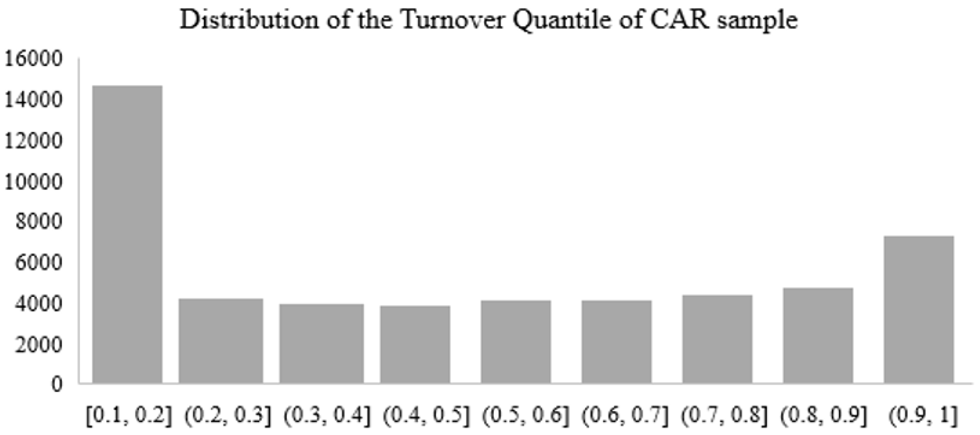
To calculate the panel data statistics, we obtained cross-sectional statistics of each quarter and took the time-series average. The crucial independent variables, D_HIGH and D_LOW, are included but not presented in the table because they are dummy variables. In these two samples, the formation period is (−5, −1), and the reference period is (−55, −6). If the average daily turnover of the formation period exceeds the 80th quantile of the average daily turnover time series of the 10-week reference period, D_HIGH is marked as 1. If the average daily turnover of the formation period is less than the 20th quantile of the reference period, D_LOW is marked as 1. This is traditional in the literature:
Akbas (
2016) uses 20% as the threshold to determine D_HIGH and D_LOW values;
Gervais et al. (
2001) use 10% as the threshold.
Table 3 presents the time-series averages of summary statistics of dependent and independent variables in each quarter. Panel A describes the SUE sample. SUE is equal to the difference in EPS between quarter q and quarter q-4 divided by the price per share in quarter q-4. It is presented in percentage form. Panel B shows the statistics for the CAR sample. CAR is defined as the average compounded return of the stock around the earnings announcement date subtracted by that of the market. Both samples span 10 years, 40 quarters from 2008 Q1 to 2017 Q4. CAR is also presented in percentage form. Other control variables are also included in both panels. To determine logSIZE, we multiplied the price per share by the share number. logBM is the log of the ratio of the book value to the equity market value. Defining the earnings announcement date as day 0, we denote the stock return over the period (−61, −12) as RETR and the stock return over the period (−6, −2) as RETF. These are both presented as percentages. TURNR is the average turnover for the same period as RETR. IVOL is the standard deviation of daily return over the period (−11, −2). Since D_HIGH and D_LOW are dummy variables, they are not included and are replaced by QTL. QTL is the quantile of the average turnover of the formation period in the average turnover of the reference period and is presented in percentage form.
All variables are quite similar except SUE and CAR. The mean of SUE is 0.125% and that of CAR is −0.090%. This indicates that the two methods capture different parts of the earnings surprises. SUE captures more information about firm fundamentals, and CAR better reflects the opinions of market participants.
Moreover, the correlation between SUE and CAR is quite low. Since the stock pool of the SUE sample is a subset of that of the CAR sample, we use the stock lists of the SUE sample as the pool and calculate the correlation coefficients between SUE and CAR. As observed in
Table 4, the correlation coefficient of the whole time period is about 0.03, and the time-series average of the quarterly correlation coefficients is 0.057. The low correlation suggests that current cash flow might not be an important factor for investors to determine the value of their stocks. This is also different from the situation in the United States.
Livnat and Mendenhall (
2006) report that the correlation between SUE and CAR is around 0.2 for the United States stock market.
4.2. Portfolio Analysis
RETVOL and TURN express differences of opinion of the market in the form of price and relative quantity. The periods are the 10-day periods (−10, −1) prior to the earnings announcement date. The correlation coefficients between the whole time series of RETVOL, TURN, and QTL of stocks in the CAR sample are displayed in
Table 5.
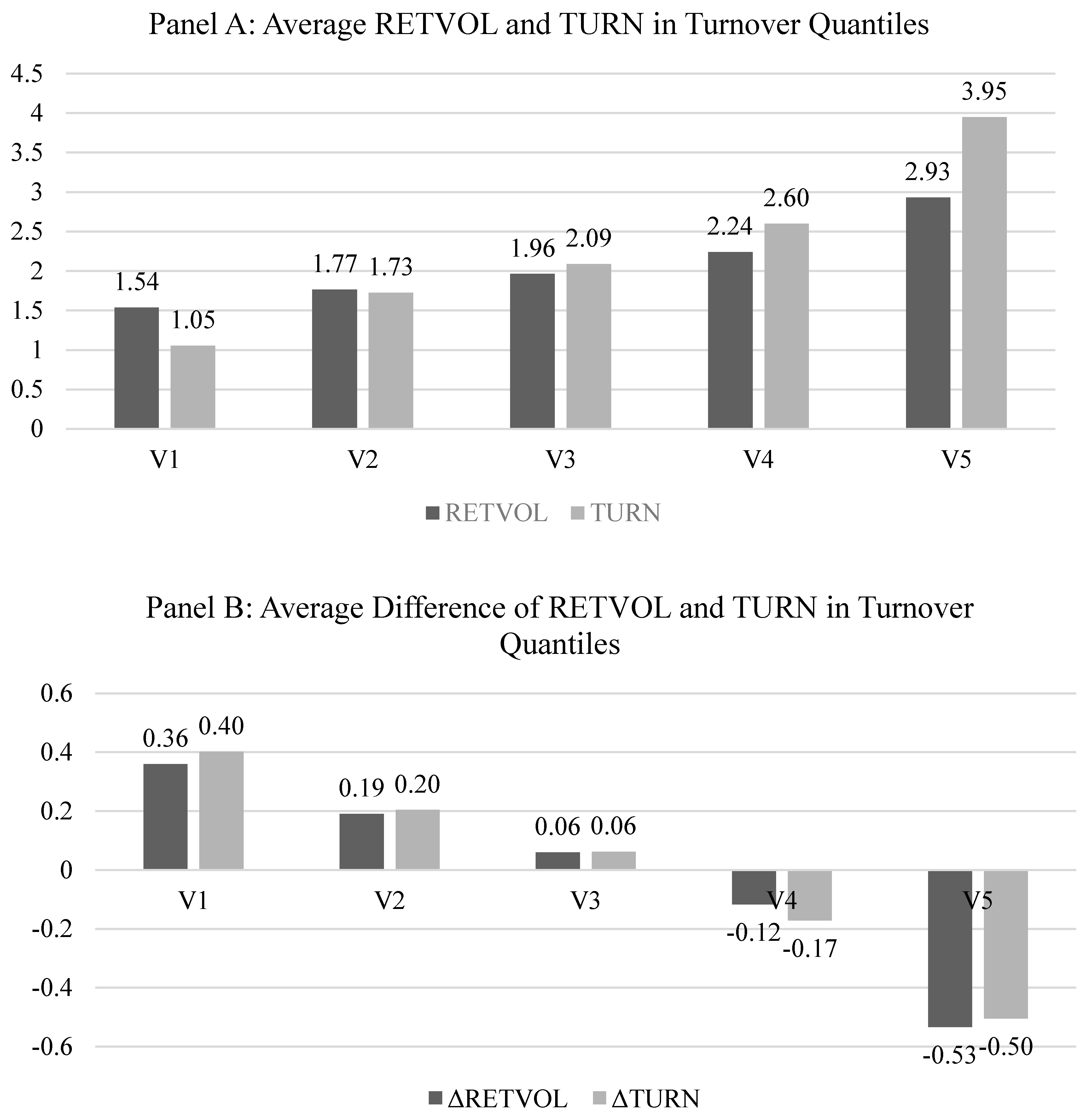
To further explore the relation between divergence of opinion and extreme trading volume, stocks in the CAR sample are analyzed by portfolio type. In each quarter, stocks fall into five categories, V1 to V5, according to QTL. The stocks with quantile of average daily turnover (QTL) from 0.1 to 0.2 fall into V1; QTL from 0.3 to 0.4, V2; QTL from 0.5 to 0.6, V3; QTL from 0.7 to 0.8, V4; and QTL from 0.9 to 1.0, V5. All stocks marked as D_HIGH fall into V5, and all stocks marked as D_LOW fall into V1. and represent the differences over period (1, 10) and period (−10, −1), reflecting the change in divergence of opinion close to the release of the earnings announcement.
Panel A of
Figure 3 shows a linear pattern. Stocks with higher QTL tend to experience a higher degree of divergence of opinion than those with lower QTL. Both trends of RETVOL and TURN substantiate the explanation that stocks with greater divergence of opinion also tend to have higher volume.
Panel B provides additional support for this explanation. Opinions concerning stocks with higher divergence of opinion would decline around the earnings announcement date. However, stocks with a relatively lower difference of opinion tend to experience a divergence of opinion around the earnings announcement date.
This pattern of divergence of opinion around the earnings announcement date helps to explain the regression results of the CAR sample, the reason for the positive signal of unusually low trading volume, and the negative signal of unusually high trading volume.
Figure 3 displays time-series averages of the measure for divergence of opinion for portfolios. Stocks are classified into five groups to represent five intervals of turnover quantiles. In panel A, RETVOL is the standard deviation of excess daily return relative to the market return over the (−10, −1) window prior to the earnings announcement date. TURN is the average daily turnover over the same period as RETVOL. TURN and
are multiplied by 100 in order to fall in the similar range of RETVOL and
. In panel B,
is the difference between the RETVOL over the (1, 10) window and the (−10, −1) window. We used the CAR sample for this analysis, which includes 1283 stocks and is larger and more complete than the SUE sample.
4.3. Estimation
4.3.1. Regression for the CAR Sample
Since individual effects exist for each firm, we use a fixed effects model to take individual effects into account. In
Table 5, the dependent variable is CAR. Fixed effect regressions are performed. To present the results more clearly, CAR and CARlag values are multiplied by 100 and denoted as CAR’ and CARlag’. RETR and RETF are multiplied by 100 and denoted as RETR’ and RETF’. Linear transformation does not change the results or the significance of the regressions. Both estimates of the two-way fixed effect regression and the one-way fixed effect regression for D_HIGH are negative and significant at the 1% level, while the estimates of the two-way fixed effect regression and the one-way fixed effect regression for D_LOW are both positive and significant at the 5% level.
This result is different from that predicted for the United States market and refutes the explanation of visibility, which claims that an extremely high trading volume would increase the visibility of the stock, leading to a rise in the stock prospects of optimistic holders. However, the unusually high volume indicates a wide divergence of opinion about the prospects of the stock. Due to short-sale constraints, the prices of these stocks are upwardly biased according to
Miller’s (
1977) theory. Therefore, stocks may experience negative return around the earnings announcement date if divergence of opinion subsides, which is the reason for the negative coefficient of D_HIGH. Stocks with increased divergence of opinion also experience a positive return, which explains the positive coefficient of D_HIGH.
In conclusion, the results shown in
Table 5 confirm that a change in difference of opinion leads to a movement in price close to the earnings announcement date. In this process, an unusual trading volume indicates the degree of divergence of opinion and signals the direction of the change of price, which could be reflected by cumulative abnormal return.
Table 6 presents the fixed effect regression results of the CAR panel data. The first column represents the two-way fixed effect regression, fixing the time as well as the individuals. The second column is the one-way fixed effect regression, fixing the time only. CAR’ is computed by subtracting the average compounded return of the market from that of the stock around the earnings announcement date and then multiplying by 100. CARlag’ is the CAR’ value from the previous quarter. D_HIGH and D_LOW are dummy variables. These variables are equal to 1 if the daily average turnover of the formation period is in the top or bottom 20% of the 10-week daily average turnover series; otherwise they are 0.
4.3.2. Regression for the SUE Sample
Similar to the regression performed on the CAR sample, SUE and SUElag are multiplied by 100 and denoted as SUE’ and SUElag’. Also, RETR and RETF are multiplied by 100 and denoted as RETR’ and RETF’. In the data presented in
Table 7, it is obvious that the coefficients of D_LOW are both negative. For both two-way and one-way fixed effect regressions, this value is statistically significant at the 10% level. Stocks with an unusually low trading volume ahead of the earnings announcement date are prone to lower standard unexpected earnings, which means deteriorated cash flow quality. This effect was not explained by firm size, book-to-market ratio, institutional ownership, trading volume, stock return, return volatility, or SUE in the previous quarter.
However, the coefficient of D_HIGH remains insignificant for stocks in China’s market. This is the same finding as that of
Akbas (
2016) for stocks in the United States. The fact that high volume stocks do not play an informational role in predicting surprises in a firm’s cash flows could be explained by high divergence of opinion. Market participants have different expectations of stock prospects, so unusually high trading volume does not have strong predictive power.
D_LOW is accompanied by less divergence of opinion and a consensus about relatively lower standard unexpected earnings. Thus, it could be concluded that unusually low trading volume contains unfavorable information about the future cash flow of the stock. However, after the EPS of a specific quarter is disclosed, the market digests this piece of information, and there may be an overshoot of the stock price, leading to positive return. This is consistent with the positive coefficients of D_LOW in the CAR’ regressions.
Table 7 presents the fixed effect regression results of the SUE panel data. The first column shows the two-way fixed effect regression, fixing the time as well as the individuals. The second column is the one-way fixed effect regression, fixing the time only. SUE equals the difference in EPS between quarter q and quarter q-4 divided by the price per share in quarter q-4. SUElag’ is the SUE’ in the previous quarter. D_HIGH and D_LOW are dummy variables. They are equal to 1 if the daily average turnover of the formation period is in the top or bottom 20% of the 10-week daily average turnover series; otherwise they are equal to 0.
4.4. Alternative Definition of Unusual Trading Volume
To check the robustness of the regressions above, we repeated the regressions by using different reference periods and formation periods to define new values of D_HIGH and D_LOW. Other variables, RETF’, RETR’, TURNR, and IVOL were also adjusted according to the new parameters. RETF’ and RETR’ represent the return over the formation period and the reference period, respectively, and are multiplied by 100. TURNR is the return over the reference period. The window of IVOL is twice the length of the formation period and ends on the day immediately prior to the earnings announcement date.
Table 8 presents the respective coefficients of D_HIGH and D_LOW in the case of alternative unusual trading volume definitions. The first and the second columns in the panel specify the new definitions of reference period and formation period. For example, (−65, −11) means we take the 55-day period, ending 11 days prior to the earnings announcement date, as the reference period. The parameter for calculating RETR’, D_HIGH, and D_LOW is adjusted accordingly. The coefficients of D_HIGH and D_LOW and their p-values are presented respectively for the SUE panel and the CAR panel.
We extended the windows of the reference period and the formation period. The results are presented in
Table 8 and suggest that the coefficient of an unusually low trading volume in the SUE regression remain statistically significant at a slightly lower significance level as the window is extended. As for the CAR sample, the coefficient for unusually high trading volume retains statistical significance at the 1% level, while that for unusually low trading volume, in general, remains statistically significant only at a higher significance level (10%). Generally speaking, the relation between unusual trading volume and earnings surprises is robust.
4.5. Robust Hausman Test
To provide a statistical rationale of using fixed effects estimation rather than random effects estimation, we do a robust Hausman test proposed by
Wooldridge (
2010). Specifically, we use bootstrap approach to calculate the variance of the difference between
and
. The results are presented in
Table 9.
The robust Hausman test strongly rejects the null hypothesis that the difference between two estimates are not systematic. Therefore, it is better to use the fixed effects model instead of the random effects model.
5. Conclusions
In this study, we investigated the relationship between an unusual trading volume and earnings surprises in China’s market, a market in which short-selling constraints are strictly enforced, and market efficiency is lower than that in developed countries. In terms of stock return, stocks with unusually low trading volumes tend to experience positive returns, and stocks with unusually high trading volume are more prone to have negative returns around the earnings announcement date. This could be explained by
Miller’s (
1977) theory that the price of stocks with a higher divergence of opinion is upwardly biased. In China’s market, stocks with an unusually high trading volume typically have higher divergence of opinion prior to the earnings announcement date and are likely to experience convergence of opinion around that date, leading to relatively lower returns compared to the market. The situation is opposite for stocks with an unusually low trading volume.
Our analysis reveals that unusually low trading volume contains negative information about firm fundamentals, as measured by standard earnings surprise. According to
Diamond and Verrecchia (
1987), in a market with short sale constraints, informed agents choose not to trade if they privately receive bad news. Low trading volume is also related to low divergence of opinion. Positive return is a correction of the overshoot caused by consensus opinion of the stock’s poor future cash flow.
The relationship between an unusually low trading volume and cumulative abnormal return (CAR) is robust in relation to changing definitions of the reference period and the formation period, as well as different definitions of unusually high or low trading volume or other control variables like RETF, RETR, TURNR, and IVOL. The relationship between unusually low trading volume and standard unexpected earnings (SUE) is also robust.
Our findings have important implications on portfolio management and policy making. Unusual high trading volume before the earnings announcement date indicates high opinion divergence of investors. However, the returns on a portfolio with lower opinion divergence are always higher than those with higher divergence. Therefore, when formulating trading strategies, investors should choose individual stocks with lower divergence to minimize the risks of portfolios and maximize profits. Besides, investors should know that the impact of opinion divergence is different during bull and bear periods. Divergence of opinions and short-selling restrictions are important features of the Chinese A-share market. The huge fluctuation of stock price caused by divergence of opinions and short-selling restrictions has a negative impact on the sustainable development of the Chinese financial market since investors are unable to make investment decisions based on companies’ fundamentals. Therefore, we propose the following policy recommendations. First, it is essential to improve the investors’ structure and establish the concept of long-term value investment. Due to the disparity of investors’ education background and information, there is supposed to be a higher divergence of opinions. Therefore, it is also necessary to raise the proportion of institutional investors. Second, we suggest that the Chinese government establish a short-selling mechanism to allow for greater degree of adaptability in the stock markets. Finally, it is important to improve information disclosure and prevent insider trading. Asymmetric information can cause dramatic fluctuations in stock prices, and sufficient information disclosure provides investors with more transparency, which would narrow divergence of opinions.
Our study demonstrates how stock markets in developing countries like China can be different than those in developed ones like the U.S. Another topic worth investigating is how generalizable this result could be in other developing societies such as India and Vietnam, which could be one of the directions for future research. Although empirical research abounds, theory on the interaction of opinions, trading and earnings is less developed, and remains for future research.


