Risk Return Trade-Off in Relaxed Risk Parity Portfolio Optimization

Abstract

This paper formulates a relaxed risk parity optimization model to control the balance of risk parity violation against the total portfolio performance. Risk parity has been criticized as being overly conservative and it is improved by re-introducing the asset expected returns into the model and permitting the portfolio to violate the risk parity condition. This paper proposes the incorporation of an explicit target return goal with an intuitive target return approach into a second-order-cone model of a risk parity optimization. When the target return is greater than risk parity return, a violation to risk parity allocations occurs that is controlled using a computational construct to obtain near-risk parity portfolios to retain as much risk parity-like traits as possible. This model is used to demonstrate empirically that higher returns can be achieved than risk parity without the risk contributions deviating dramatically from the risk parity allocations. Furthermore, this study reveals that the relaxed risk parity model exhibits advantageous traits of robustness to expected returns, which should not deter the use of expected returns in risk parity model.

1. Introduction

While fund management and portfolio optimization have been extensively studied in literature, one aspect known as risk parity has gained considerable traction. Risk parity was developed to remove the uncertainty of estimated returns and to protect against losses associated with portfolio concentration. A proactive risk parity approach has been shown to reduce draw-downs over more risky strategies, which gives the strategy its importance, as touted by Qian (2005); Maillard et al. (2010) and Lee (2011). However, the increase in draw down protection limits upside growth in strong bull markets, so it is commonly used to protect from large losses rather than to seek greater returns. The conservativeness may be too steep for some practitioners, so it would be useful for a practitioner to increase returns while still retaining to some degree the benefits of risk parity allocations. In this regard, one can still guard against unexpected market downturns by diversifying the risk across all the assets.

1.1. Portfolio Optimization and Risk Parity Background

Since the inception of modern portfolio theory (MPT) and mean-variance optimization (MVO), introduced by Markowitz (1952) academic literature has expanded with insights into improvements to this fundamental basis of portfolio allocation. Choosing the best portfolio of assets and their individual weights, x, out of all possible portfolios being considered is the essence of portfolio optimization. Each asset has an expected return, $\mu$, and a standard deviation of returns, $\sigma$, computed from historical data. The relationship between the assets is governed by the variance–covariance (VCV) matrix of asset returns $\mathsf{\Sigma }$, which indicates the correlations between assets that a solver uses to minimize the portfolio variance, ${\sigma }_p$. MVO portfolios seek the lowest amount or risk for a given level of return and is represented in Model (1). This model uses both performance aspects and risk aspects to achieve the optimal asset allocations by considering the trade-off between risk and return that is governed by the asset correlations.

$$\begin{array}{cc}\hfill \underset{x}{\min }& \frac{1}{2}{x}^T\mathsf{\Sigma }x\hfill \\ \hfill \mathrm{s}.\mathrm{t}.& \mu x^T\ge r\hfill \\ \hfill & \mathbf{1}{x}^T=1\hfill \\ \hfill & x\ge 0\hfill \end{array}$$

(1)

When achieving the minimum variance (MV) for a target return the optimization does not consider the individual risk of assets, only the total risk of the portfolio. Due to this feature of the MVO, portfolios can be allocated into a few assets as the framework concentrates into assets with low volatility or vice versa for maximum return (Markowitz 1952). This is the leading criticism of mean-variance portfolios. The uncertainty of the estimated parameters can lead to undiversified portfolios in terms of asset weights and risk. MVO portfolios are typically high in estimation error and are sensitive to inputs due to the estimated expected returns as shown by Best and Grauer (1991) and Chopra and Ziemba (1993). This leads to unstable portfolios depending on the quality of the estimated parameters and it is shown that small changes in the input estimated returns can lead to significant changes to asset allocations (Merton (1980); Black and Litterman (1992)).

1.1.1. Shift to Risk Based Ideology

The confounding effects of the uncertainty in MVO has led to the study of techniques that try to eliminate the need for estimated parameters, mainly expected returns and covariances. As shown by Chopra and Ziemba (1993), the estimated VCV matrix causes less instability then the estimated expected returns and it is suggested by Chopra and Frahm and Wiechers (2011) that simply removing the need for estimated expected returns from the optimization is possible and leads to primarily risk-based optimizations that are more stable. In MVO, this equates to the minimum-variance portfolio which itself concentrates into the assets with the lowest volatility. However, this still produces undiversified portfolios with even lower returns.

The available methods of asset allocation have evolved primarily from extensions and changes to the original mean-variance framework and efforts have been made to correct for the MVO’s tendency to produce over-concentrated portfolios. This has led to the development of equal-risk contribution (ERC) portfolios as measured by the standard deviation (Maillard et al. (2010); Roncalli (2014)) without the need to incorporate expected returns and results in diversification.

The risk contribution of an asset is defined by the product of its weight in the portfolio and its marginal risk contribution (MRC). As discussed in Bai et al. (2016) and confirmed by Roncalli and Weisang (2016), Euler’s Decomposition can be used to decompose the total portfolio risk measure, standard deviation ${\sigma }_p^2$, into individual asset risk contributions ${\sigma }_i$, where n is the number of assets in the portfolio. The assets marginal risk contributions will define how individual assets are approached in the optimization beyond just using the total portfolio risk which is asset agnostic in an MVO.

By enforcing a risk bound on each asset as explored by Haugh et al. (2015) and Cesarone and Tardella (2017) or in this case, equal risk budgets, every available asset is present in some magnitude, ensuring diversity. The differences between risk contributions are minimized with a strategy commonly known as risk parity optimization, which leads to this desired diversification trait. Risk parity optimization protects against over-concentration into individual assets; it is the forced construction of diversified portfolios in which resources are allocated based on the measure of risk where all assets contribute equal risk ${\sigma }_i$ (2), rather then equal weight. Risk-based portfolios do not require an explicit estimation of asset expected returns and the sum of the asset absolute risk contributions (ARC) equates to the total portfolio risk (3).

$$\begin{array}{c}\hfill {\sigma }_i\left(x\right)=\frac{x_i{\left(\mathsf{\Sigma }x\right)}_i}{\sqrt{x^T\mathsf{\Sigma }x}}=\frac{\sqrt{x^T\mathsf{\Sigma }x}}{n}where\forall ii=1...n,n=\#\mathrm{of}\mathrm{assets}\end{array}$$

(2)

$$\begin{array}{ccc}\hfill {\sigma }_p& =& \sqrt{x^T\mathsf{\Sigma }x}=\sum _1^n{\sigma }_{i}where\forall ii=1\dots n\hfill \end{array}$$

(3)

Various methods exist for producing risk parity portfolios as explored by Maillard et al. (2010); Feng and Palomar (2015) and Bai et al. (2016), including the least squares approach and the log barrier methods. Risk parity overcomes the drawbacks of Markowitz portfolios by attempting to reduce the reliance on noisy estimated parameters which may mislead the optimization to rely on unreliable estimated asset returns. Risk parity optimization eliminates the expected returns from the model entirely. Traditionally, the risk parity formulation is a least squares fourth-order objective problem as composed in model (4). The risk contribution of each asset is represented by $x_i{\left(Qx\right)}_i$ and is compared to another assets risk contribution denoted by $x_j{\left(Qx\right)}_j$. The model will compare risk contribution of each asset with every other asset and reach an objective value of 0 indicating all risk contributions are the same.

$$\begin{array}{cc}\hfill \underset{x}{\min }& \sum _{i=1}^n\sum _{j=1}^n{(x_i{\left(\mathsf{\Sigma }x\right)}_i-x_j{\left(\mathsf{\Sigma }x\right)}_j)}^2\hfill \\ \hfill \mathrm{s}.\mathrm{t}.& {\mathbf{1}}^{T}x=1\hfill \\ \hfill & x_i\ge 0\hfill \end{array}$$

(4)

This polynomial objective is non-linear and non-convex and concerns over its numerical complexity are raised when considering additional constraints in the model. To alleviate these concerns, Lobo et al. (1998) discuss the applications of a second-order cone programming (SOCP) model and a clear implementation to risk parity is shown by Mausser and Romanko (2014) who use an equivalent SOCP formulation as it appears in Model (0). Model (4) is reformulated by transformation of the constraints into cone constraints and a transformation of the objective into linear form. This SOCP formulation is an epigraph of the least squares method, but it is readily and efficiently solvable by quadratic solvers due to its convex nature (Ben-Tal and Nemirovski (1998); Alizadeh and Goldfarb (2003)) and is more friendly and flexible to additional constraints to deal with the expected return information. The SOCP model is suitable since the model is using the standard deviation of returns as the risk measure which maps to the second order constraints (7) and (8). Alternative risk measures are not compatible with this model.

$$\begin{array}{cc}\hfill \mathrm{Model}\left(0\right)\underset{x}{\min }& \psi -\gamma \hfill \end{array}$$

(5)

$$\begin{array}{cc}\hfill \mathrm{s}.\mathrm{t}.& {\zeta }_i={\left(\mathsf{\Sigma }x\right)}_i\mathrm{i}=1\dots \mathrm{n}\hfill \end{array}$$

(6)

$$\begin{array}{cc}\hfill & x^T\mathsf{\Sigma }x\le n{\psi }^2\hfill \end{array}$$

(7)

$$\begin{array}{cc}\hfill & x_i{\zeta }_i\ge {\gamma }^2\mathrm{i}=1\dots \mathrm{n}\hfill \end{array}$$

(8)

$$\begin{array}{cc}\hfill & {\mathbf{1}}^{T}x=1\hfill \end{array}$$

(9)

$$\begin{array}{cc}\hfill & x_i,{\zeta }_i\ge 0\mathrm{i}=1\dots \mathrm{n}\hfill \end{array}$$

(10)

$$\begin{array}{cc}\hfill & \psi ,\gamma \ge 0\hfill \end{array}$$

(11)

As the linear objective of the SOCP formulation approaches zero, the risk contribution between each asset becomes equal. Each asset’s absolute risk contribution (ARC), denoted ${\gamma }_i$, is compared to the average risk of the portfolio, $\psi$. The average risk of the portfolio $\psi$ in (7) is an upper bound on the risk contribution of any individual asset and dictates that any one asset’s risk contribution should be equal to or less than the average risk. The average risk of the portfolio equates to an equal risk magnitude, so the objective is effectively enforcing the risk parity allocations. To facilitate this, the lower bound of an individual asset’s risk contribution is $\gamma$, enforcing that $\psi$ ≥ $\gamma$. The total risk contribution of each asset is computed using the asset’s MRC and asset weight through constraints (6) and (8), respectively. When $\psi$ = $\gamma$, it is obvious that it is a risk parity portfolio and the model becomes a minimization of the difference between these two risk values. The SOCP effectively minimizes the difference between each asset’s risk contribution and the average risk of the portfolio instead of comparing each asset to another, reducing the computational complexity along the way. Lastly, constraint (9) defines the common portfolio budget requirements.

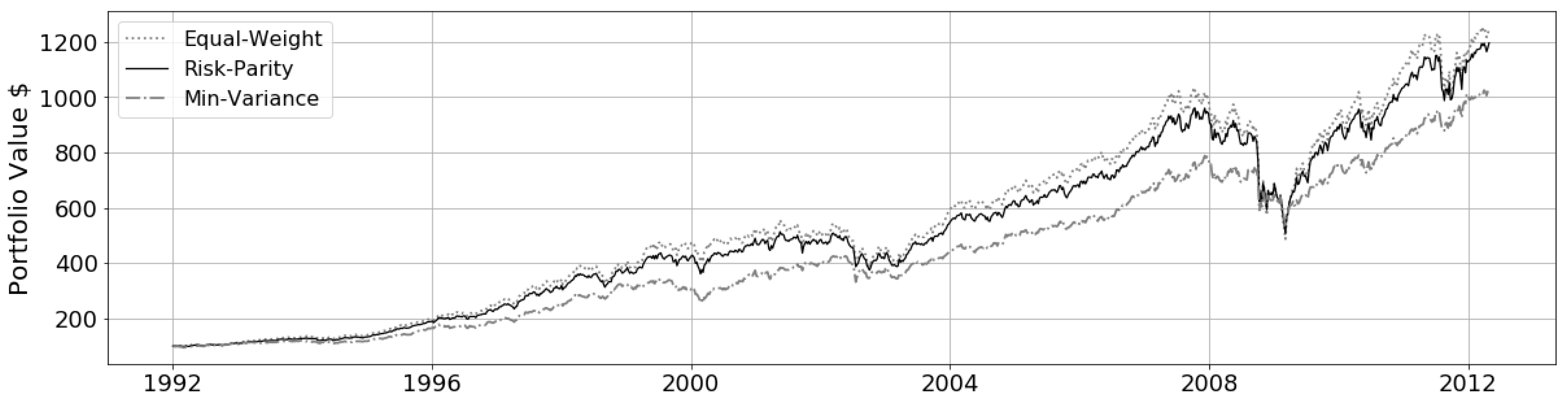
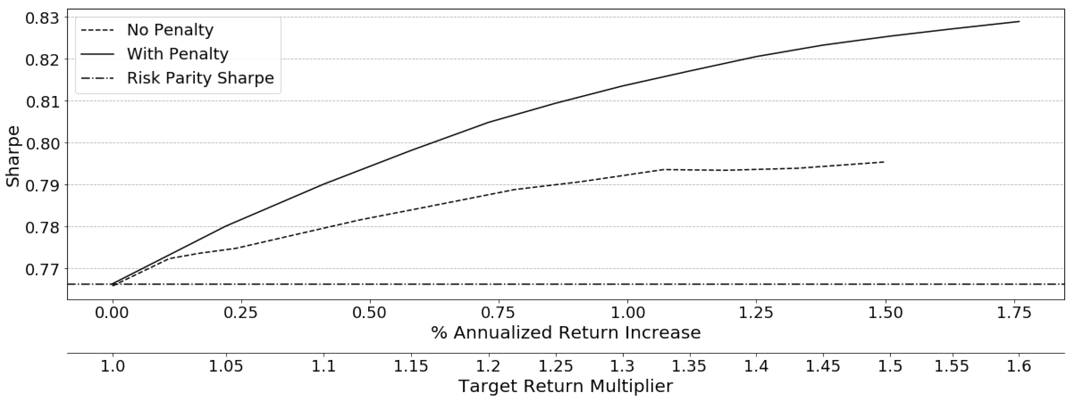
Due to the ability to enforce diversity, risk parity achieves neither minimum risk nor maximum returns and it is shown by Maillard et al. (2010) that the performance lies between the minimum-variance and the equal weight portfolio. An in-sample analysis was conducted over a 20 year period on a 50-asset set and plotted in Figure 1. This plot demonstrates how risk parity takes advantage of riskier assets much like an equal weight portfolio and produces returns above minimum variance. This trend is reversed in market crashes seen immediately following the 2008 market crash where equal weight and risk parity portfolio losses converge below the minimum variance portfolio due to added weight in the higher risk assets.

Risk parity is both a meaningful and effective approach to portfolio construction. It has removed expected returns to alleviate the concerns of instability and balance return with diversification of risk, thereby avoiding concentration into risky assets.

1.1.2. Motivation and the Utilization of Return Estimates

Few studies exist on the introduction of performance aspects into risk parity. Roncalli (2014) shows how to build risk parity portfolios that depend on the expected returns by using a risk measure that incorporates expected returns rather than just the standard deviation of realized returns. Roncalli demonstrates this risk-budgeting technique where each asset has a performance and volatility aspect and the risk budget limits define the weight allocations based on that trade-off. Much like the risk parity optimization, when a risk budget is greater than zero, it must hold the asset in some weight, enforcing diversity. His model serves to benefit from the additional information that the expected returns provide to find more accurate risk parity portfolios. He finds that some merit exists in the balance of risk-based allocation and performance-based allocation, which this paper seeks to exploit. Lee (2011) had a similar sentiment prior, rejecting that risk parity improves efficiency and arguing that it is the starting point in the absence of stronger investment views which Roncalli supplements with expected returns; the model presented in this paper is driven from this inclusion.

Feng and Palomar (2015) explore different risk parity formulations and apply different performance objectives and risk measures, such as volatility, VaR and CVaR, to a successive convex optimization to solve for long and long/short portfolios. They show the non-convexity of the various risk parity formulations that lead to the necessity of a numerical algorithm to solve to find the most optimal solutions. This gives rise to the use of a second order epigraph of the least-squares risk parity by Mausser and Romanko (2014) as the basis for our model. This second-order cone program (SOCP) model permits the addition of further open-faced constraints, such as the target return used to force a violation, and is solvable via modern quadratic solvers in the long-only domain, alleviating some of the numerical difficulties for practical implementation.

Ardia et al. (2018) develops a metric to optimize the balance between performance and risk aspects. The metric measures concentration of weight and how much it diverges from the risk contributions, measuring the mismatch between performance and risk contributions. They use the framework to optimize other strategies to match the underlying performance of risk parity in terms of volatility and return and not to specifically enhance returns as is the aim of this study. Along with Ardia, this paper infuses the performance and risk aspects to achieve this. Rather than finding an optimal mean-variance trade-off the notion of targeting near risk parity, portfolios are introduced to capture the useful traits of risk parity to the highest degree possible or passing control to the practitioner. To alleviate the mean-variance aspect, Perchet et al. (2015) recognizes that driving the optimization on the VCV matrix converges an MVO towards minimum-variance and confirms that using the diagonal of the VCV matrix converges towards equal risk allocations instead, due to a less aggressive driving matrix. Methods are implemented in this study that utilize these findings to incorporate the estimated expected returns to tilt the standard risk parity portfolio away from its current conservative allocation and seek greater returns.

1.1.3. Parameter Uncertainty and Robust Optimization

Rejecting the statistical uncertainty in models using estimation is impossible; however, significant works have been produced to depart from the simpler agnostic data-driven descriptive statistics which need to be mentioned here. Both the sample mean return and sample covariance matrix are estimated using traditional first and second order methods over the historical returns of each asset. The introduction of estimated expected returns into the risk parity model raises concerns over its estimation error as well. Estimated parameters from raw data have a degree of uncertainty, which can render the optimal solutions a poor fit to the model. There have been multiple approaches introduced to deal with estimation error (Black and Litterman (1992); Roncalli (2014); Jorion (1986); DeMiguel and Nogales (2006); bauwens2006multivariate), the most popular approaches being autoregressive conditional heteroscedastic models, shrinkage methods and robust optimization, as discussed by Goldfarb and Iyengar (2003) and Tütüncü and Koenig (2004).

Conditional heteroscedastic models relax the assumption of constancy of the covariance matrix and instead follow a flexible dynamic structure (Engle 2002). Using many assets requires a multi-variate generalized autoregressive conditional heteroscedasticity (M-GARCH) model that forecasts changes to the volatility of financial time series in the short term (Bauwens et al. 2006). The proposed model will utilize a longer term rolling procedure that estimates the covariance over a 3-year period. Holding a portfolio over the 6–12-month period before re-balancing may not add significant value to the model and the proposed model avoids the added complexity. Alternatively, shrinkage methods (Ledoit and Wolf (2003); Kwan (2011)) improves the conditioning of the covariance matrix. Sample covariance matrices are subject to estimation error of the kind most likely to perturb a mean-variance optimizer. Instead it uses a weighted average of the sample and target covariance matrices to generate a near-true covariance matrix by pulling the most extreme coefficients towards a more central value and systematically reducing estimation error (Ledoit and Wolf 2004). Two aspects arise here—this is usually required when there are insufficient observations of the underlying variables to the number of assets Daniels and Kass (2001). This is not the case in the proposed model analysis where there are 15x the number of observations of assets. Secondly, the risk parity-like behavior of the proposed model naturally limits the extremes in variance allocation which counteracts the underlying purposes of using shrinkage methods. The strongest argument against using either method is the naturally risk limiting behavior of the risk parity like model that avoids concentration into high return assets and sub-sequentially the uncertainty that comes with them.

Robust optimization seeks to optimize a portfolio to the worst-case realization of the estimated parameters. Strong discussions on the traction of robust portfolios are authored by Ceria and Stubbs (2006), Fabozzi et al. (2007), Kim et al. (2014b) and Kim et al. (2014a). Santos (2010) confirms that the methods by Ceria et al. and Tütüncü and Koenig (2004) produce better portfolios in terms of the Sharpe ratio and turnover when compared to mean-variance portfolios. This indicates that robust optimization is an effective way to alleviate problems with estimation errors in returns.

Much like minimum variance and equal weight portfolios, risk parity portfolios are assumed to be robust due to the diversification of risk. Poddig and Unger (2012) show that the outcome of risk parity portfolios are far less influenced by estimation errors than MVO portfolios. This paper demonstrates that robust optimization adds a layer of complexity to the optimization, which sees little benefit (Section 5.6). By using risk parity as the underlying optimization for the enhanced model, it is argued that it retains some inherent robustness to estimated expected returns and, to some degree, nullifies the effects of uncertainty. Further details can be found in Bertsimas et al. (2011), including a comprehensive list of literature on robust optimization.

1.2. Purpose and Contributions

Protecting from the downside with diversified portfolios limits the upside, resulting in poor performance in stable growth markets. The purpose is to develop a tool which relaxes the risk parity optimization by allowing risk parity to be violated while biasing the solver towards risk parity. This will improve upon the conservative nature of the model, but not dramatically so, asserting that finding near risk parity portfolios will provide improved bull market performance without a dramatic increase in risk.

Risk parity was created to overcome two aspects, first to improve the diversification over the common MVO and so reduce the negative effects from estimated parameter uncertainty. The second is to overcome the effects of cap weighted portfolios, such as with the SP500, which is already well diversified. The SP500 is the backbone of investing, where trillions of dollars are traded, so by diversifying and avoiding cap weighted concentrations, this will save it from a 2001 dot-com style bubble through risk budgeting. There are two main arguments that must be addressed to achieve the research goals. The returns must be added back into the risk parity optimization to increase the aggressiveness of the model and yield higher returns, which can concentrate the risk allocations motivating the second aspect, driving the risk contributions back towards equal risk to avoid this concentration. There is no SOCP based model with a return goal that hosts extra constructs to keep the risk allocations near risk parity. There are works that incorporate the potential use of returns to improve risk measures but nothing to affect the resulting risk allocations specifically. This paper proposes the incorporation of a return goal into a second-order-cone program (SOCP) model of a risk parity optimization and include a computational construct to obtain near risk parity portfolios to retain as much risk parity like traits as possible.

This paper is organized as follows. First, Section 1 introduces the background on portfolio optimization and various strategies that set the foundation for the proposed model. Section 2 introduces the methods and evaluation metrics. Section 3 describes the relaxed risk parity model and introduces the rationale for the relaxation technique employed. Section 4 details the risk contribution characteristics of the model and parameter optimization in-sample. Section 5 presents the computational experiments including the out-of-sample performance, relative model performance and risk to return properties of the model. Lastly, Section 6 discusses the model’s results and makes conclusions towards the research question.

2. Methods and Data

Risk-parity is a strategic allocation for long-term protection from negative market events. With this in mind, the model is considered under a long investment horizon; including the periods post the 2001 dot-com crash and the 2008 financial meltdown. The most recent bull market from 2009 to 2018 is examined since it represents the current financial environment and regulatory practices that have changed since the 2008 financial crash. The analysis uses a diversified set of 50 US Stocks (

Table 1. Summary of assets and estimated annualized properties between 1992 –2018.

Consumer Disc.			Consumer Staple			Healthcare			Information Tech.			Utilities
	$\mathit{\mu }$	$\mathit{\sigma }$		$\mathit{\mu }$	$\mathit{\sigma }$		$\mathit{\mu }$	$\mathit{\sigma }$		$\mathit{\mu }$	$\mathit{\sigma }$		$\mathit{\mu }$	$\mathit{\sigma }$
F	12.1	15.5	KR	14.8	10.9	MRK	11.0	9.8	IBM	12.1	10.1	ED	9.9	6.6
GT	10.2	16.3	MO	17.2	9.5	PFE	13.7	9.5	MSI	14.7	14.9	ETR	11.2	7.8
FL	14.1	15.6	CL	14.0	8.4	LLY	13.6	9.8	HPQ	15.3	13.3	DTE	11.7	7.2
DIS	14.5	10.1	KO	10.7	8.1	BMY	10.5	9.6	TXN	26.0	14.6	CNP	11.1	10.9
MCD	16.2	8.2	PEP	12.0	7.6	JNJ	13.3	7.5	XRX	8.9	15.1	AEP	10.9	8.1
PG	13.2	8.0							QCOM	32.4	18.1	LNT	11.1	7.3
Energy			Financial			Industrial			Material			Telecommunication
	$\mathit{\mu }$	$\mathit{\sigma }$		$\mathit{\mu }$	$\mathit{\sigma }$		$\mathit{\mu }$	$\mathit{\sigma }$		$\mathit{\mu }$	$\mathit{\sigma }$		$\mathit{\mu }$	$\mathit{\sigma }$
CVX	13.7	8.4	AON	15.5	10.4	BA	17.5	11.1	PPG	14.6	9.6	T	10.2	9.1
MRO	11.8	12.9	BK	17.7	11.6	LMT	15.6	9.2	AA	10.9	14.4	VZ	11.1	8.5
OXY	15.6	10.6	AXP	18.9	11.9	MMM	13.6	8.2	DD	31.0	29.4	S	10.2	17.3
XOM	11.2	7.6	C	16.1	18.3	CAT	21.1	12.0	IP	9.0	12.3
HAL	16.2	15.3	WFC	18.1	12.5	DE	19.8	11.8

) as constructed in Costa and Kwon (2019) selected from the S&P 500 index encompassing the ten GICS industry sectors. The 10-year US T-Bill rate is interpreted as the risk-free rate and is used to compute the ex-post Sharpe ratio.

The Sharpe ratio as introduced by Sharpe (1994), is a financial ratio that measures the excess return per unit of deviation commonly referred to as the risk adjusted return. This ratio indicates the quality of the return based on how much risk was taken on and generally a higher Sharpe ratio is desired. The ex-post Sharpe ratio is computed in this study from the annualized mean and standard deviation of excess returns based on underlying weekly return and risk-free rate data.

The portfolio turnover detailed by Santos (2010) indicates how much the portfolio components have changed over some period to have the optimal portfolio. This value is an indirect measurement of the magnitude of the transaction cost and is expected to be greater then zero since this model employs an active strategy. Lastly, to evaluate how closely the portfolio aligns with the risk parity allocations the Euclidean distance between each assets ARC to the expected risk parity risk contributions is computed. A mean squared error (MSE) measure provides a single comparable distance value henceforth referred to as distance and labeled d. A smaller distance to risk parity is desired when we violate risk parity to achieve the higher target goals.

3. Relaxed Risk Parity Model Development

This proposed model is an extension of the Mausser and Romanko (2014) risk parity SOCP with aspects from Roncalli (2014) and Perchet et al. (2015). The use of the expected return parameters is expected to yield value to the construction of near risk parity portfolios. Unlike in Roncalli’s method, the expected returns are implemented in a manner such that the optimal portfolio’s return performance can be increased. This targets enhanced returns and retains risk diversification, which is the targeted property of risk parity.

3.1. Enhanced Risk Parity SOCP Formulation

An additional target return constraint (16) is added to the SOCP model, Model (A), proposed by Mausser and Romanko (2014). The target return is needed to target returns greater than risk parity so the optimization can violate the risk parity trait by restricting the portfolio from reaching equal risk values. Terms (12)–(15) and (17) are identical to the SOCP Model (0) in Section 1.1.1, where they are discussed.

$$\begin{array}{cc}\hfill \mathrm{Model}\left(\mathrm{A}\right)\underset{x}{\min }& \psi -\gamma \hfill \end{array}$$

(12)

$$\begin{array}{cccc}\hfill \mathrm{s}.\mathrm{t}.& {\zeta }_i={\left(\mathsf{\Sigma }x\right)}_i\mathrm{i}=1\dots \mathrm{n}\hfill & \hfill & \mathrm{marginal}\mathrm{risk}\hfill \end{array}$$

(13)

$$\begin{array}{cccc}\hfill & x^T\mathsf{\Sigma }x\le n{\psi }^2\hfill & \hfill & \mathrm{risk}\mathrm{bound}\hfill \end{array}$$

(14)

$$\begin{array}{cccc}\hfill & x_i{\zeta }_i\ge {\gamma }^2\mathrm{i}=1\dots \mathrm{n}\hfill & \hfill & \mathrm{total}\mathrm{risk}\hfill \end{array}$$

(15)

$$\begin{array}{cccc}\hfill & \begin{array}{|c|}\hline {\mu }^T\mathbf{x}\ge R\\ \hline\end{array}\hfill & \hfill & \mathrm{target}\mathrm{return}\hfill \end{array}$$

(16)

$$\begin{array}{cccc}\hfill & {\mathbf{1}}^{T}x=1\hfill & \hfill & \mathrm{portfolio}\mathrm{budget}\hfill \\ \hfill & x_i,{\zeta }_i\ge 0\mathrm{i}=1\dots \mathrm{n}\hfill \\ \hfill & \psi ,\gamma \ge 0\hfill \end{array}$$

(17)

Figure 2a presents the risk allocations of the feasible risk parity solution for the risk parity SOCP. The risk parity risk contribution target can be seen as the dotted horizontal dashed line and the assets labeled X1 through X50. Choosing a return value greater then the expected risk parity return results in Figure 2b and there is a deviation from the risk parity target line for all assets while concentration occurs into a few. The model is considering the expected return as one of the drivers of the risk-return trade-off, so parallels the MVO result. This concentration of risk is due to the mean-variance aspect of the model, which does not consider the distribution of additional risk needed to achieve the target return.

Concentrated risk is counter-productive to achieving near-risk parity portfolios and their properties. Higher risk concentrations may experience more volatile behavior and see greater losses when the stability of a market is threatened. This characteristic is mitigated through the use of a risk parity optimization; however, the additional risk needs considered.

3.2. Relaxation of the Risk Parity Attribute

The SOCP is a form of relaxation itself as the least squares formulation objective is reformulated into the constraints. A feasible risk parity solution for a long only model may not exist when a change to the structural constraints of the SOCP risk parity model is imposed (Mausser and Romanko 2014). As shown by Bai et al. (2016) and Lemma 5.1, the long-only risk parity optimization has a unique solution. So, any structural changes that restrict one from reaching this solution will result in a violation of the risk parity property. This suggests the enhanced return model in Model (A) cannot find an exact risk parity solution for all target return goals R and that a relaxation is necessary to find the closest risk parity solution possible while in violation. An objective function that is as small as possible produces near risk parity results; however it is shown in Figure 2b that this is not entirely the case in the enhanced return Model (A), where concentration of risk is witnessed leading to larger objective values. The enhanced portfolio is modified with an additional regulating constraint that controls the risk concentrations, so the model coerces the risk allocations towards risk parity.

The risk parity model is relaxed by allowing the model to violate the risk parity property and produce portfolios with non-equal risk contributions. This is achieved by targeting a higher return through the additional target return constraint (16). The risk contribution of each asset is governed by constraint (18). It represents the average risk which is the risk parity value; where n is the number of assets. By increasing or decreasing this bound, control over the distribution of risk can be imposed. The relaxation is activated by applying the regulating term $\rho$ (18) to the individual asset risk bound, allowing for it to move away from the risk parity value. Constraint (18) is modified to include a regulating term $\rho$ on the asset risk bound in constraint (19). Where $\rho$ represents a change to the risk parity bound where any positive $\rho$ increases the bound. The regulating term increases the deviation between the bound and asset risk contribution, while the total objective is minimized.

$$\begin{array}{ccc}\hfill x^T\mathsf{\Sigma }x& \le & n{\psi }^2\hfill \end{array}$$

(18)

$$\begin{array}{ccc}\hfill \frac{x^T\mathsf{\Sigma }x}{n}& \le & {\psi }^2-{\rho }^2\hfill \end{array}$$

(19)

The magnitude of this regulating term $\rho$ is governed by the weights of the assets and covariance matrix, providing a passive term for the model to optimize over. The $\rho$ determines the outcome of the portfolio allocations and the distribution of risk that is enforced by limiting the risk of individual assets. This is performed through a risk minimization term based on the weights and VCV matrix of asset returns (20).

$$x^T\mathsf{\Sigma }x\le {\rho }^2$$

(20)

The regulating term provides the model a variable that increases the risk bound of each absolute risk contribution (ARC) within the model itself finding a bound that reaches the target return at the best variance possible. Imposing this structural change onto Model (A) with the addition of constraint (25) and a change to (23) results in the relaxed Model (B).

$$\begin{array}{cc}\hfill \mathrm{Model}\left(\mathrm{B}\right)\underset{x}{\min }& \psi -\gamma \hfill \end{array}$$

(21)

$$\begin{array}{cccc}\hfill \mathrm{s}.\mathrm{t}.& {\zeta }_i={\left(\mathsf{\Sigma }x\right)}_i\hfill & \hfill & -\mathrm{marginal}\mathrm{risk}\hfill \end{array}$$

(22)

$$\begin{array}{cccc}\hfill & \begin{array}{|c|}\hline x^T\mathsf{\Sigma }x\le n({\psi }^2-{\rho }^2)\\ \hline\end{array}\hfill & \hfill & -\mathrm{risk}\mathrm{bound}\hfill \end{array}$$

(23)

$$\begin{array}{cccc}\hfill & x_i{\zeta }_i\ge {\gamma }^2\hfill & \hfill & -\mathrm{total}\mathrm{risk}\hfill \end{array}$$

(24)

$$\begin{array}{cccc}\hfill & \begin{array}{|c|}\hline x^T\mathsf{\Sigma }x\le {\rho }^2\\ \hline\end{array}\hfill & \hfill & -\mathrm{regulating}\mathrm{term}\hfill \end{array}$$

(25)

$$\begin{array}{cccc}\hfill & {\mu }^T\mathbf{x}\ge R\hfill & \hfill & -\mathrm{target}\mathrm{return}\hfill \end{array}$$

(26)

$$\begin{array}{cccc}\hfill & {\mathbf{1}}^T\mathbf{x}=1\hfill & \hfill & -\mathrm{budget}\hfill \\ \hfill & x_i,{\zeta }_i\ge 0\hfill \\ \hfill & \psi ,\gamma \ge 0\hfill \end{array}$$

(27)

Comparing Figure 3a from the enhanced risk parity return from before to Figure 3b, that is using the VCV matrix in the regulating term, shows an aggressive re-allocation of risk away from the visible risk parity target line. The risk parity value has changed due to the stronger re-allocation. Increasing the target risk from the average risk of the portfolio (23) with the addition of the regulating term $\rho$ permits the risk contribution of any asset to reach the total risk of the portfolio. This lifts the upper bound considerably and gives way for the solver to achieve portfolios that have extreme risk allocations, which is undesirable. However, this is a meaningful method of control over the distribution of risk that can be utilized.

Table 2. Effect of regulating term with VCV ($\mathsf{\Sigma }$).

	Model (A)		Model (B)
Target (%)	Return	Risk	Return	Risk
25	0.393	0.145	0.393	0.145
30	0.429	0.158	0.428	0.163
35	0.461	0.187	0.460	0.192
45	0.501	0.299	0.502	0.297

shows how the addition of the regulating term using the VCV matrix does not improve the characteristics of the performance. This leads to a strategic design of the regulating term in Section 3.3.

The variance–covariance matrix in the model is measuring linear associations only. In deriving the covariance matrix a non-linear model could be used such as a non-linear shrinkage method presented by Ledoit and Wolf (2004). Investigating the risk parity-like conditions in a non-linear covariance environment is an interesting subject for further research but the traditional covariance matrix definition is suitable for an approximate distribution of risk due to the use of daily historical observations over 3 years. Instability of the covariance matrix is seen when the number of assets is near the number of historical observations, so the resulting stability becomes less of a concern when using small asset sets with many observations, as seen in this study. Larger dimensional matrices would require more advanced methods, such as shrinkage, for VCV estimation. This is complemented by the risk parity-like structure of the model which is naturally imposing diversification across the assets, which will avoid some undesirable concentration seen in the traditional mean-variance optimization when using data-driven estimations.

3.3. Regulating Term and Penalty Selection Rationale

The primary objective of the term $\rho$ is to decrease the deviations of risk contributions from risk parity when a violation to risk parity allocations occurs. Since the model attributes its behavior to the mean-variance structure that is re-introduced with the target return constraint (26), the solver will allocate any additional risk towards the assets with the highest expected returns without further consideration for risk diversification. Controlling this imbalance in the risk allocations through the additional term $\rho$ is paramount.

The weight of an individual asset in an MVO portfolio is the normalized inverse of the assets volatility which results in the vector of weights for the MVO portfolio. If left unconstrained, the weights of the MVO converge towards a minimum variance portfolio which can include short positions as discussed by Perchet et al. (2015). Applying this concept above in Model (B) has shown that that this can be too aggressive since the model is intended to converge towards equal risk allocations for risk parity. Perchet et al. (2015) studies the affect of different alternative drivers in place of the VCV matrix including an identity matrix and the diagonal of the VCV. By imposing a long-only constraint and using a diagonal matrix of asset volatilities, Perchet et al. confirms that, in a robust mean-variance optimization, the risk allocations converge towards equal risk budgets. By using the diagonal of the VCV matrix (29) in the regulating term (28) and (29), only the variances of each asset are penalized instead of all the interactions of the assets. This focuses the model on the individual asset variances to drive the magnitude of penalty on the diversification of risk.

$$\begin{array}{c}\hfill x^T\mathsf{\Theta }x\le {\rho }^{2}where\mathsf{\Theta }=diag\left(\mathsf{\Sigma }\right)\end{array}$$

(28)

$$\begin{array}{c}\hfill \left[\begin{array}{c}{x}_1\\ ⋮\\ x_i\end{array}\right]\left[\begin{array}{ccc}{\sigma }_{1,1}& \cdots & 0\\ ⋮& \ddots & ⋮\\ 0& \cdots & {\sigma }_{i,j}\end{array}\right]\begin{array}{c}\left[\begin{array}{c}{x}_1\cdots x_i\end{array}\right]=\rho \\ \\ \\ \end{array}\end{array}$$

(29)

Using $\mathsf{\Theta }$ is restricting a large portion of the total portfolio risk from being influenced by individual assets. A smaller $\rho$ restricts investing in assets whose individual assets are high. Constraint (28) is using the diagonal of the VCV which limits how much of the total portfolio variance is coming from individual variances. It is placing a limit on the total portfolio variance to avoid most of the variance being influenced by these high return assets. This further distributes the risk across the remaining lower variance assets based on the asset correlations. The model still accounts for all asset-to-asset correlations in mechanism (23), while $\mathsf{\Theta }$ in (28) is the mechanism that limits any assets with high variance from getting too much weight. As compared to using the VCV matrix in the regulating term in Figure 4a, Figure 4b uses the $\mathsf{\Theta }$ construct to further distribute the risk across the assets and closer to risk parity allocations. The risk bound target for risk parity has increased, as indicated by the dashed horizontal line, because the total portfolio risk has increased due to the restriction from finding lower variance portfolios using all available interaction effects. This must be accepted when using the relaxed risk parity optimization in this form.

The aggressiveness of the regulating term can be controlled through an additional penalty $\lambda$ in constraint (30). The degree of difference between the assets risk contributions can be impacted by changing the strength of the regulating term.

$$\begin{array}{c}\hfill \lambda x^T\mathsf{\Theta }x\le {\rho }^2\end{array}$$

(30)

Increasing the penalty $\lambda$ increases the magnitude of the regulating term $\rho$. The progression of risk allocation in Figure 5 across various penalty values is presented. Note the change in risk concentration, as the $\lambda$ multiplier is increased to 1.0. As the penalty value is increased in magnitude, the risk allocations begin too distribute further across the portfolio assets. The size of this $\lambda$ can be set to find better performing near-risk parity portfolios. Note that Figure 4b and Figure 5d both represent allocations at $\lambda =1$ and would present the same result with the same target return. However, Figure 5d is targeting a 1.2× return, so the allocations of risk are greater to achieve this goal.

The model presented is based on a naïve risk parity framework that works because of the presence of approximate risk parity constraints that translate to good diversification across the assets. This is witnessed in the results in Figure 4b—despite using the simpler data-driven second order covariance estimation approach. This is in contrast to other methods, such as M-GARCH and other shrinkage methods, which address uncertainty by estimating a new covariance matrix to limit concentration into uncertain assets. This framework is desirable because it can avoid using additional complex estimation methods, discussed in Section 1.1.3, and still achieve good diversification, thereby limiting the effects of uncertainty.

The novel implementation of this regulating term to the underlying risk parity model achieves the desired effect, which will be referred to as a relaxed risk parity portfolio. This study rationalizes risk distribution towards risk parity as being the greatest priority to the practitioner in order to gain its desirable traits.

3.4. The Relaxed Risk Parity Model

The relaxed risk parity model is formulated using (19) and (30). This is a passive relaxation as it does not provide direct control over the deviation of the risk allocations from risk parity. Rather, the solver best distributes the risk allocations in a way that also inherently minimizes the risk for the given target return and distribution requirements. This model can be interpreted as an enhanced risk parity optimization, subject to a risk diversification constraint that targets the risk parity allocations allowing for a near risk parity portfolios.

The SOCP model by Mausser and Romanko (2014) is changed with the addition of the return constraint (36) and the penalized risk regulating term (35) to produce Model (C). The feasible space of this model is limited to a long-only domain where the weights x are positive and the regulating term $\rho$ is also positive in order to increase risk dispersion to approach risk parity. A practitioners first decision is to select the underlying portfolio of assets. It is assumed that the investors desire a long-term strategy and have pre-determined the asset set. Any modification to the assets is done at the discretion of the investor. This model does not indicate investment opportunities or provide decisions whether to limit the weight of an asset to near zero. Rather, this model actively includes all assets.

$$\begin{array}{cc}\hfill \mathrm{Model}\left(\mathrm{C}\right)\underset{x}{\min }& \psi -\gamma \hfill \end{array}$$

(31)

$$\begin{array}{cccc}\hfill \mathrm{s}.\mathrm{t}.& {\zeta }_i={\left(\mathsf{\Sigma }x\right)}_i\hfill & \hfill & -\mathrm{marginal}\mathrm{risk}\hfill \end{array}$$

(32)

$$\begin{array}{cccc}\hfill & x^T\mathsf{\Sigma }x\le n({\psi }^2-{\rho }^2)\hfill & \hfill & -\mathrm{risk}\mathrm{bound}\hfill \end{array}$$

(33)

$$\begin{array}{cccc}\hfill & x_i{\zeta }_i\ge {\gamma }^2\hfill & \hfill & -\mathrm{total}\mathrm{risk}\hfill \end{array}$$

(34)

$$\begin{array}{cccc}\hfill & \lambda x^T\mathsf{\Theta }x\le {\rho }^2\hfill & \hfill & -\mathrm{penalized}\mathrm{regulating}\mathrm{term}\hfill \end{array}$$

(35)

$$\begin{array}{cccc}\hfill & {\mu }^T\mathbf{x}\ge R\hfill & \hfill & -\mathrm{target}\mathrm{return}\hfill \end{array}$$

(36)

$$\begin{array}{cccc}\hfill & {\mathbf{1}}^T\mathbf{x}=1\hfill & \hfill & -\mathrm{budget}\hfill \\ \hfill & x_i,{\zeta }_i\ge 0\hfill \\ \hfill & \psi ,\gamma \ge 0\hfill \end{array}$$

(37)

When the individual asset risk contributions are used in the model through the variance–covariance matrix to generate the marginal risk contributions (32) they become indefinite and are technically non-convex even if the variance–covariance matrix is positive-semi-definite (PSD). A global minimum is not guaranteed; however, this is not the purpose of the model. Risk parity in the long and short domain is known to have issues with convexity and are only very close to finding the most optimal solutions. Due to the additional constraints added to this long-only relaxed risk parity model, the convexity is still lost. In practice, as long as solutions can be generated that target the near-risk parity portfolios the computational ability of the model is less of a concern.

3.5. Adaptive Target Return

The model requires a target return goal R to enforce an enhanced return above the nominal risk parity portfolio. The model must first compute the expected return and covariances of asset returns using the historical data along with the expected risk parity return. An intuitive target return approach is considered using a target return (38) based on a multiple m of the historical risk parity return. The reader should note, that when an optimization period has a negative risk parity return, the return is adjusted towards zero based on the underlying absolute return value to avoid searching for lower returns. This is achieved via the maximum selector between the expected risk parity return and zero.

$$\begin{array}{c}\hfill \mathrm{R}=m·max(\mathrm{E}{\left[\mathrm{x}\right]}_{\mathrm{RP}},0)\mathrm{where}m\in \mathrm{I}\mathrm{R}\ge 1.0\end{array}$$

(38)

This method is used to target an enhanced risk parity return by ensuring the goal is higher than the most recent known risk parity return. The adaptive target return model adjusts the periods target according to the previous known return which, to some degree, reflects the current market environment. It does not guarantee the highest return, but it improves the feasibility and does not require a specific return goal from the practitioner, which is difficult to estimate. Both in-sample and out-of-sample analyses will be conducted by varying the range of the target return multiplier from 1.0x to 1.8x, where 1.0x indicates the risk parity portfolio.

4. In-Sample Risk Contribution Analysis

The efficient frontier comprises of a set of optimal portfolios that result in the highest expected return for the given level of risk (Markowitz 1952). Risk parity portfolios do not lie on the efficient frontier due to the risk diversification property that limits finding portfolios with the minimum risk or maximum return. A new frontier that lies somewhere below the mean-variance efficient frontier that aligns with the risk parity portfolio is expected and presented in Figure 6 and Figure 7. When m = 1.0x it is obvious that the model produces a risk parity portfolio and aligns with that associated risk and return. The relaxed risk parity frontier in both plots moves almost equally to offset from the MVO efficient frontier but takes on more risk due to the forced diversification, which is why it appears less efficient. Giving up efficiency is okay—it allows the model to find the near risk parity portfolios—which is the priority over minimizing risk.

By increasing the penalty strength values beyond $\lambda =1$, the underlying model deviates from the risk parity, as seen when $\lambda =100$. The portfolios find more extreme concentrations and efficiency is traded for better dispersion of risk towards risk parity. This behavior is pronounced in a bull market where the model takes advantage of the better performing assets to find higher returns. The bull market period frontier represented in Figure 7 reveals that the benefits of the model are strengthened during strong markets. An increasing penalty moves the relaxed risk parity frontier away from the risk parity frontier producing higher returns for the same level of risk. This is a positive trait, the closer the portfolio is to risk parity the less the risk parity traits and variance are in conflict, so a properly chosen penalty lambda can take advantage of some of the better performing assets. Conversely, as the return target R becomes more aggressive, the portfolio losses efficiency, such as when m = 1.6x. At higher returns, there is a greater deterioration of the model’s performance due to concentration of assets. Above this point, the model’s performance aspects take precedence and the penalty $\lambda$ loses its effectiveness to target near-risk parity portfolios. The distance from risk parity is affected by both the target return and the penalty strength and can be observed in Figure 8 spanning various target returns. This plot indicates the average distance to risk parity in-sample for the increasing target return multiplier m.

For this model there is a decrease in distance from risk parity, as seen in Figure 8, when $\lambda >0$. The portfolio becomes nearer to risk parity with $\lambda \le 1$ up until a 1.6x target return goal. Within this range of return and penalty $\lambda$, the practitioner can expect an improvement in the risk parity properties for an enhanced portfolio over an un-regulated model. The plot reveals at $\lambda =100$ that the underlying risk parity model is violated at a target return multiplier m = 1.0x, where the distance to risk parity $d_{M}SE$ is much greater than zero. This is confirmed by the data in

Table 3. In-Sample MSE Distance to RP with increasing $\lambda$—1997–2018.

Target	$\mathit{\lambda }$ = 0		$\mathit{\lambda }$ = 0.5		$\mathit{\lambda }$ = 1		$\mathit{\lambda }$ = 100
m	Sharpe	${\mathit{d}}_{\mathit{MSE}}$	Sharpe	${\mathit{d}}_{\mathit{MSE}}$	Sharpe	${\mathit{d}}_{\mathit{MSE}}$	Sharpe	${\mathit{d}}_{\mathit{MSE}}$
1.0x	0.622	0	0.622	0	0.622	0.003	0.633	0.036
1.1x	0.691	0.08	0.681	0.071	0.679	0.072	0.683	0.080
1.2x	0.74	0.145	0.721	0.134	0.718	0.136	0.717	0.152
1.4x	0.762	0.271	0.753	0.265	0.752	0.269	0.748	0.302
1.6x	0.725	0.404	0.738	0.408	0.736	0.413	0.734	0.429
1.8x	0.649	0.565	0.668	0.56	0.667	0.561	0.667	0.567
2.0x	0.569	0.756	0.584	0.75	0.584	0.751	0.585	0.753

Note: Rolling Horizon = 6 months, $\lambda$ = 0.2, Look-back = 3 years.

and indicates that the model cannot find risk parity portfolios at the same target return as risk parity with high lambda values. Using $\lambda =100$ would never be advised or used in practice and is here to demonstrate a natural limit to the parameter before the underlying risk parity is affected—this appears to be $\lambda =1$ from Table 3. This agrees with the plot in revealing values of $\lambda$ less then one to produce superior results.

Penalty increases the result in a reduction to the Sharpe ratios in Table 3. This is due to the reduction in allocation in high-risk high return assets and a minor increase in variance due to some concentrations required to meet the target return. The distance measure $d_{MSE}$ is tabulated in Table 3 and

Table 4. In-Sample MSE Distance to RP with increasing $\lambda$—2009–2018.

Target	$\mathit{\lambda }$ = 0		$\mathit{\lambda }$ = 0.5		$\mathit{\lambda }$ = 1		$\mathit{\lambda }$ = 100
m	Sharpe	${\mathit{d}}_{\mathit{MSE}}$	Sharpe	${\mathit{d}}_{\mathit{MSE}}$	Sharpe	${\mathit{d}}_{\mathit{MSE}}$	Sharpe	${\mathit{d}}_{\mathit{MSE}}$
1.0x	1.331	0	1.331	0	1.335	0.005	1.389	0.037
1.1x	1.377	0.075	1.395	0.052	1.397	0.051	1.441	0.054
1.2x	1.399	0.130	1.425	0.097	1.428	0.096	1.471	0.095
1.4x	1.396	0.230	1.424	0.194	1.428	0.194	1.460	0.203
1.6x	1.363	0.328	1.338	0.313	1.340	0.317	1.345	0.333
1.8x	1.306	0.436	1.246	0.448	1.242	0.452	1.237	0.460
2.0x	1.126	0.610	1.133	0.614	1.132	0.615	1.132	0.616

Note: Rolling Horizon = 6 months, $\lambda$ = 0.2, Look-back = 3 years.

as the distance to risk parity for a 20 year period of 1997 to 2018 and a bull market period 2009–2018, respectively.

Both tables indicate that a penalty $\lambda <1$ produces smaller distances to risk parity and improved Sharpe ratios indicate that enhancing risk parity is possible using portfolios near risk parity. The Sharpe ratios do not always improve over an un-regulated model ($\lambda$ = 0) at higher target returns, but this is not the primary goal, rather the reduction in distance to risk parity is. Specifically, in a bull marker period in Table 4, the Sharpe ratio can be seen to improve up until the target m = 1.2x when $\lambda =0.5$.

This structural study of the model demonstrates that an increasing penalty strength $\lambda$ can positively affect the efficient frontier by reducing the total portfolio risk. For high target returns, this penalty approaches the mean-variance portfolio with a higher distance to risk parity where the desirable risk parity properties degrade. When the model is calibrated and used within a reasonable range of enhanced return and $\lambda$ penalty strength shows a stronger result than the risk parity portfolio.

Parameter Optimization

A range exploration strategy is employed for model parameter estimation. To facilitate the out-of-sample analysis, the hyper-parameter $\lambda$ is fixed for a penalty strength that achieves a balance between distance to risk parity and performance. A grid-search is carried out across increasing penalty strength and target return multipliers. As determined in Section 4, the penalty $\lambda$ affects how the relaxed risk parity model frontier approaches the efficient frontier. Reasonable gains can be made with appropriate tuning between zero and one. Values of $\lambda >1$ are too strong and concentrate risk through over-penalization. A strong penalty over-penalizes each individual risk asset and results in portfolios that are no nearer to risk parity. A $\lambda <$ 1 value indicates that a reduction in strength of the regulating term achieves a better result.

Table 5. Single period with increasing return multiplier and penalty value $\lambda$.

	1.0x		1.1x		1.2x		1.4x		1.6x		1.8x
$\mathit{\lambda }$	Sharpe	${\mathit{d}}_{\mathit{MSE}}$	Sharpe	${\mathit{d}}_{\mathit{MSE}}$	Sharpe	${\mathit{d}}_{\mathit{MSE}}$	Sharpe	${\mathit{d}}_{\mathit{MSE}}$	Sharpe	${\mathit{d}}_{\mathit{MSE}}$	Sharpe	${\mathit{d}}_{\mathit{MSE}}$
0	1.331	0	1.377	0.075	1.399	0.13	1.396	0.23	1.363	0.328	1.306	0.436
0.1	1.331	0	1.394	0.061	1.398	0.069	1.421	0.195	1.348	0.309	1.261	0.451
0.2	1.331	0	1.398	0.058	1.398	0.058	1.425	0.194	1.347	0.306	1.273	0.43
0.3	1.331	0	1.396	0.053	1.426	0.097	1.422	0.194	1.339	0.309	1.257	0.439
0.4	1.331	0	1.395	0.052	1.425	0.097	1.423	0.194	1.338	0.311	1.251	0.443
0.5	1.331	0	1.395	0.052	1.425	0.097	1.424	0.194	1.338	0.312	1.248	0.446
0.6	1.331	0	1.395	0.052	1.426	0.097	1.425	0.194	1.338	0.313	1.246	0.448
0.7	1.331	0.001	1.395	0.051	1.427	0.097	1.426	0.194	1.339	0.314	1.245	0.449
0.8	1.332	0.003	1.396	0.051	1.427	0.097	1.426	0.194	1.339	0.315	1.244	0.45
0.9	1.332	0.004	1.396	0.051	1.427	0.097	1.427	0.194	1.339	0.316	1.243	0.451
1	1.335	0.005	1.397	0.051	1.428	0.096	1.428	0.194	1.34	0.317	1.242	0.452

results indicate a low penalty strength of $\lambda =0.2$ in Model (B) and produces the smallest distance to risk parity across the various return levels and will be used in the remainder of this study.

The optimal rolling horizon size and look-back period for the out-of-sample analysis is determined through a grid-search of possible values. The results indicate that the shorter training period produces superior Sharpe ratios to longer training periods and that the bi-annual re-optimization achieves the same level of performance as the annual horizon at less turnover. This procedure indicates that a 6-month rolling time horizon with a 3-year look-back period produces the best results. It is generally accepted that a shorter training period will better reflect the current market conditions, which is desirable to control the risk allocations. For brevity, the details are excluded.

5. Out-of-Sample Computational Analysis

5.1. Rolling Horizon Out-of-Sample Analysis Procedure

A fixed term re-balancing rolling horizon framework outlined by (DeMiguel et al. 2009) is used with varying target return goals m for the out-of-sample analysis in Section 5. This leads to the following generalized two stage model implementation, as outlined in Algorithm 1. The rolling window horizon length is selected to take advantage of the time series characteristics, which will better reflect the most recent market environments for some look back periods. The adaptive target return from Section 3.5 updates each re-optimization period using the 3-year training period with 6-month rolling horizon.

Algorithm 1: Multi Period Out-of-Sample Optimization.

As the rolling horizon moves each defined period forward, the parameter estimation window follows so only the newest periods of data and parameter estimates are used. The portfolios are held constant over the next defined out-of-sample period and the performance of each portfolio is evaluated. This is continued until the entire available time period is consumed by the rolling time horizon. Each roll of this optimization is performed using Gurobi (Version 8.01) with python on an i7-8550u 1.8 GHz 4-Core 16 GB Windows 10 system and solves in a matter of minutes with n = 50 assets.

5.2. Out-of-Sample Performance

The two-stage rolling algorithm in Section 5.1 is used to evaluate the out-of-sample performance of Model (C). The model is applicable to any time frame applied to it bearing in mind that it has sufficient trailing data for the look back period. The out-of-sample analysis uses a 3-year look-back period with weekly data to estimate the expected returns, VCV matrix and the expected risk parity return prior to the start of the first rolling period. The analysis is performed over 20 years using a 6-month rolling horizon that begins January 1997 and ends mid-2017, consisting of a total of 23 years of weekly return data across 40 investment periods. A fixed 6-month rolling period is used that aligns with potential real-world strategies1. The comparison of the proposed model to existing strategies as used by Lohre et al. (2014) is disregarded in this work as Lohre demonstrates the meaningfulness of a maximum diversified portfolio. It is well understood that the rationale and positioning of the risk parity portfolio within the field is meant to achieve a conservative return and is understood to have lower Sharpe ratios. The relative out-of-sample portfolio value to the nominal risk parity portfolio value is depicted in Figure 9 and the performance is tabulated in

Table 6. Annualized Out-of-Sample Performance—Proposed Model.

Target m	Return	% $\Delta$ R	Volatility	% $\Delta$ Vol	Sharpe	Distance	% Turnover
1.0x	11.37	–	15.11	–	0.788	0.000	8.3
1.2x	12.07	7	15.28	1	0.822	0.250	20.5
1.4x	12.55	12	15.66	3	0.833	0.479	33.9
1.6x	13.06	16	16.19	6	0.839	0.727	47.3

.

The results indicate that the annualized total return over the investment horizon across various market conditions does indeed improve, including the Sharpe performance. The returns improvements are not dramatic, which reflects the conservative nature of using the risk parity model in the first place. Moderately improving beyond risk parity in a predicable manner is witnessed with a consistent lift in cumulative return for the increase in target return multiplier m.

A closer look at the relative cumulative returns period by period in Figure 9 across the different market conditions shows an acceleration of growth during periods of stable market conditions, such as in 2004–2009, leading to greater wealth accumulation. Alternatively, an acceleration of losses is witnessed when the target return is high due to a more concentrated portfolio. This is attributed to the adaptive target return, which will increase the target return in each optimization period as the bull market continues. The change in annualized return and annualized volatility in Table 6 reveals that the return is increasing at a greater magnitude then the volatility shown by examining $\%\Delta$ R and $\%\Delta$ Vol. This increase in target return will increase the distance to risk parity in bull markets to capture the well performing assets; however, aggressive target return multipliers will increase the distance to risk parity beyond a reasonable amount, leading to a dramatic loss in risk parity traits. Care must be taken to balance to choose the values of the parameters used.

These higher return multipliers subsequently reduce the risk parity properties in bull markets, which is desirable. This is apparent in Figure 9, im which, during 2000 and mid-2012, the loss in portfolio value during a correction is amplified. The subsequent 3-year periods after market shocks in Figure 9, specifically 2002 to 2005 and 2009 to 2012, indicate that the relative value stays consistent when volatile periods are included in the parameter estimation period. The resulting relative growth in portfolio wealth is forgone as the model reverts closer to the risk parity weighting. Risk parity fails to capitalize on changing estimated returns and the results here reinforce the notion that including the estimated returns in this controlled manner can moderately capitalize on strong market conditions and still seek risk parity traits.

5.3. Does the Proposed Model Achieve Better Out-of-Sample Performance?

The return characteristics in

Table 7. Annualized out-of-sample performance.

Target	Mean-Variance			Enhanced Risk Parity			Relaxed Risk Parity
m	Return	Risk	Sharpe	Return	Risk	Sharpe	Return	Risk	Sharpe
1.0x	9.85	13.33	0.773	11.23	15.44	0.766	11.37	15.11	0.788
1.2x	10.33	13.61	0.793	11.59	15.66	0.778	12.07	15.28	0.822
1.4x	10.96	14.13	0.810	12.14	16.15	0.791	12.55	15.66	0.833
1.6x	11.78	14.69	0.835	12.73	16.87	0.795	13.06	16.19	0.839

reveal improvements to the performance. The MVO produces the best Sharpe ratios as expected because it is not restricted from finding the lowest possible variance of the portfolio. The additional regulating term $\rho$ used to find near risk parity portfolios reduces this risk, improving the Sharpe ratio over the enhanced risk parity model. From

Table 8. Out-of-sample distance to risk parity.

Target	Mean-Variance		Enhanced Risk Parity		Relaxed Risk Parity
m	${\overline{\mathit{d}}}_{\mathit{MSE}}$	${\mathit{\sigma }}_{\mathit{MSE}}$	${\overline{\mathit{d}}}_{\mathit{MSE}}$	${\mathit{\sigma }}_{\mathit{MSE}}$	${\overline{\mathit{d}}}_{\mathit{MSE}}$	${\mathit{\sigma }}_{\mathit{MSE}}$
1.0x	1.781	0.600	0.000	0.000	0.000	0.000
1.2x	1.804	0.593	0.411	0.173	0.331	0.137
1.4x	1.857	0.582	0.710	0.295	0.598	0.258
1.6x	1.949	0.567	0.996	0.428	0.880	0.410

, the enhanced risk parity clearly has a reduction in distance and distance volatility against the MVO model, which is the expected outcome. Furthermore, a strong reduction in distance to risk parity is witnessed again with the inclusion of the risk regulating term $\rho$. As the risk allocations approach near risk parity portfolios, a reduction in the distance volatility, ${\sigma }_{MSE}$, indicates that large deviations have been reduced across the investment horizon, resulting in further diversification of risk.

The relaxed risk parity model has near equivalent Sharpe performance to an MVO but at an improved annualized return with smaller distances to risk parity across all target returns studied. Higher returns are shown for the enhanced target return model but at an increase in risk. Including the risk regulating term with the enhanced risk parity model improves the risk diversification and the results indicate a moderate improvement to the annualized return. This aligns with the hypothesis of this study, that better performing out-of-sample portfolios in terms of Sharpe ratio and distance to risk parity are possible with near risk parity portfolios.

5.4. Reversion to Risk Parity in Volatile Market Conditions

The distance from risk parity indicates to what degree the portfolio may retain risk parity characteristics. Progression along the investment horizon reveals that the model reverts to risk parity allocations, Figure 10, following significant market shocks and confirms the findings from Figure 9.

During periods of market distress, the adaptive target return approach produces target returns that are below what the risk parity return can achieve due to the depreciation of expected return estimates in the look-back period. The instability in returns results in the model disregarding the mean-variance trade-off and forming the optimization with only the risk characteristics; ultimately reverting the model back to the risk parity weighting. The mean-variance conflict becomes negligible and any additional information from the expected returns is not considered. This can be seen during 2002 to 2004 in which the portfolio’s relative performance follows in line with the risk parity portfolio after only the 2 year training period beyond the crash. This acts as a guard against concentrated portfolios and inherently and indirectly adds a robust layer to the model since it does not dramatically lose value below the risk parity portfolio in a market correction. The single-period risk, return and distance to risk parity is computed to demonstrate this trait. It is obvious from the results in

Table 9. Reversion to risk parity for low target returns.

Target m	Risk	Sharpe	Distance
1.0x	15.11	0.788	0.000
0.2x	15.11	0.788	0.000
0.8x	15.11	0.788	0.000
1.2x	15.28	0.822	0.137

that target return goals with a multiplier between 0.2x and 0.8x (indicating a target goal less then the risk parity return) results in the risk parity allocation, which is equivalent to the 1.0x target return multiplier.

Although useful, there is a lag in the models reaction to the crash due to the look-back period length. If the market stays volatile for long periods it will be at risk parity but will not capture short periods of high volatility due to the averaging effect of the mean asset returns over the historical training period. This translates to a slower reaction to the start of bull markets forgoing some possible early gains. This model is purely raw-data-driven and does not incorporate predictive indicators to correct for this lag that change the models parameters, based on predicted market conditions, such as in Costa and Kwon (2019). Capturing market changes lags the current market events by the size of the look-back period and rolling horizon. These two parameters can be decreased in size to capture current market events sooner, since no predictive indicators are being used, but some lag must still be accepted.

5.5. Cost Versus Benefit of Relaxation for Enhanced Portfolios

The increase in volatility is used as an approximate measure of how much risk that a practitioner takes on to enhance the returns from the nominal risk parity result. Conducting a test using a 6-month rolling horizon with a range of target return multipliers from 1.0x through 1.8x reveals Figure 11, depicting the target return to portfolio volatility increase. The curve indicates that the increase in volatility has a non-linear relationship with return. The results from both the enhanced risk parity model, Model (B), and the relaxed risk parity model, Model (C), are included. The results show that the use of the additional risk regulating term is justified for the proposed model and that a modest increase in return can actually lead to portfolios with equivalent risk as the risk parity portfolio itself. As the risk parity properties are lost with higher returns, the cost increases dramatically. This reinforces the idea that near-risk parity portfolios can yield better returns without a dramatic cost to the risk parity traits.

A look at the average distance to risk parity for each re-optimization period in Figure 12 indicates the loss of risk parity properties over the horizon. It is obvious that targeting near risk parity portfolios lowers the distance to risk parity, as compared to no penalty, and that the loss in risk parity traits over a horizon for each target multiplier is quite consistent. The linear relationship indicates that the risk parity properties are lost at a predictable rate with enhanced returns. The distance from risk parity has an almost equivalent volatility to the underlying risk parity portfolio at 1.15x return, as revealed in Figure 11.

The Sharpe ratio progression in Figure 13 of the relaxed risk parity is always greater then the un-regulated Model (B), confirming better Sharpe characteristics with near risk parity portfolios for increasing target return multipliers opposing the in-sample result in which there is a decrease at higher target returns. In all analysis cases, the relaxed risk parity model out-of-sample consistently out-performs the nominal risk parity model and the more concentrated Model (B).

5.6. Inherent Robust Traits for Handling Uncertainty

It is well understood in the literature that the dependence on estimated parameters—namely the expected return and VCV matrix of asset returns—leads to estimation error because they are determined from sample estimates (Fama and French 1993). Chopra and Ziemba (1993) extend this idea by showing that the uncertainty in the estimated expected returns are much more significant than the estimated covariances (Best and Grauer (1991); Michaud (1989)), indicating that improving these estimates would dramatically improve the portfolio’s stability.

It is shown here that the relaxed risk parity model inherently combats perceived instabilities that might arise without resorting to additional robust optimization methods. Risk parity alone is not a robust model but could exhibit the traits of a robust model. A robust model embeds the uncertainty into the model design and accepts the uncertainty into the optimization as a deterministic variability to the estimated return. It is generally used to keep the solver away from noisy estimated parameters and prevent too much weight being applied to assets with very high expected returns and high standard errors. It provides solutions immune to uncertainty by using the worst-case scenario of the estimated return parameter for each asset facilitated by allowing the solver to choose some value of expected return around the estimated return to use as the true return. The implementation is done through applying an uncertainty set around the expected return estimates and scaled by the standard error of the asset returns.

Robustness is added to Model (C) through the addition of an ellipsoidal uncertainty set (45) around each estimated return, as described by Tütüncü and Koenig (2004). Model (D) applies a regulatory term and sizing parameter to the estimated returns (44) of the portfolio. Two regulating terms with penalties are seen in Model (D), one acting on the risk as $\rho$ and the other on the return as $\kappa$.

$$\begin{array}{cc}\hfill \mathrm{Model}\left(\mathrm{D}\right)\underset{x}{\min }& \psi -\gamma \hfill \end{array}$$

(39)

$$\begin{array}{cccc}\hfill \mathrm{s}.\mathrm{t}.& {\zeta }_i={\left(\mathsf{\Sigma }x\right)}_i\hfill & \hfill & -\mathrm{marginal}\mathrm{risk}\hfill \end{array}$$

(40)

$$\begin{array}{cccc}\hfill & x^T\mathsf{\Sigma }x\le n({\psi }^2-{\rho }^2)\hfill & \hfill & -\mathrm{risk}\mathrm{bound}\hfill \end{array}$$

(41)

$$\begin{array}{cccc}\hfill & x_i{\zeta }_i\ge {\gamma }^2\hfill & \hfill & -\mathrm{total}\mathrm{risk}\hfill \end{array}$$

(42)

$$\begin{array}{cccc}\hfill & \lambda x^T\mathsf{\Theta }x\le {\rho }^2\hfill & \hfill & -\mathrm{penalized}\mathrm{regulating}\mathrm{term}\hfill \end{array}$$

(43)

$$\begin{array}{cccc}\hfill & {\mu }^T\mathbf{x}-\kappa \ge R\hfill & \hfill & -\mathrm{target}\mathrm{return}\hfill \end{array}$$

(44)

$$\begin{array}{cccc}\hfill & {ϵ}^{2}x\mathsf{\Omega }x\le {\kappa }^2\hfill & \hfill & -\mathrm{uncertainty}\mathrm{set}\hfill \end{array}$$

(45)

$$\begin{array}{cccc}\hfill & {\mathbf{1}}^T\mathbf{x}=1\hfill & \hfill & -\mathrm{budget}\hfill \\ \hfill & x_i,{\zeta }_i\ge 0\hfill \\ \hfill & \psi ,\gamma ,\kappa \ge 0\hfill \end{array}$$

(46)

It is obvious that the regulating terms for both the risk, $\rho$, and the return, $\kappa$, parallel each other in structure. However, they serve different purposes. Notably, the return regulating term is driven by the standard error $\mathsf{\Omega }$ (47) and a defined confidence term $ϵ$ (48), which determines the size of the uncertainty set. The $ϵ$ variable is the inverse cumulative chi-square distribution at a given confidence level, denoted by $\alpha$, typically 95% or 99%. The distance determined using the standard error of the estimation is proportionally enlarged using the $ϵ$ sizing parameter. A tighter confidence is indicated by a higher confidence level, which produces a larger ellipsoid that indicates a greater confidence that the true value is within the ellipsoid.

$$\begin{array}{ccc}\hfill \mathsf{\Omega }& =& diag\left(\mathsf{\Sigma }\right)/NwhereN=\#samples\hfill \end{array}$$

(47)

$$\begin{array}{ccc}\hfill ϵ& =& {\chi }^2\left(\alpha \right)\to ϵ={\chi }^2(0.95,n)\hfill \end{array}$$

(48)

When comparing the results from the relaxed risk parity in Model (C) to a robust version of Model (D) at a 95% confidence level, the improvement is negligible with limited feasibility at higher target returns. This result indicates that the model is already seeing some robust traits. Model (C) has a constrained feasible space and therefore is seeing lower performance then an MVO in-sample. This is a purposeful design trait to restrict reaching the MVO allocations, so as to achieve the diversity of near-risk parity portfolios. The proposed model exhibits quasi-robust properties due to the similarity in structure to the ellipsoidal uncertainty set constraints. The frontier in Figure 14 indicates the feasible range of Model (D). This in-sample result is paralleled in the out-of-sample performance in Figure 15, where changes to the performance are negligible. The robustification works against the risk parity target by concentrating risk into assets, which explains the small improvement to the return in

Table 10. Annualized out-of-sample performance.

Strategy	Return	Volatility	Sharpe
Risk Parity	11.23	15.44	0.765
Relaxed Risk Parity	12.04	15.62	0.805
Robust Relaxed Risk Parity	12.15	15.63	0.810
Mean-Variance	11.37	14.59	0.809

.

The level of confidence that is feasible in the out-of-sample result is only 5%. This is, in part, due to a smaller optimization sample size, which increases the $ϵ$ value and with it the uncertainty set size. An aggressive confidence penalizes the returns beyond capabilities of satisfying the target return and, therefore, renders the model infeasible. Targeting near-risk parity portfolios improves the performance over risk parity alone and exhibits some robust traits. Including the ellipsoidal uncertainty set into the target return sees negligible improvement to the models out-of-sample performance. The presence of this relaxed risk parity has some robust advantages, but not equivalent to traditional robust optimization. The robust model still has better performance on a percentage point basis, but the relaxed risk parity model helps alleviate some of the concerns from expected returns by absorbing some of the uncertainty, just not all of it. By limiting the risk in the model, the risk parity trait organically limits the concentration into assets with higher uncertainty. The weight and risk allocations in

Table 11. Summary Statistics of Relaxed Risk Parity versus Robust Risk Parity.

	Weight Allocations			Risk Allocations
	Relaxed Risk Parity	Robust Risk Parity		Relaxed Risk Parity	Robust Risk Parity
Std Dev	0.0114	0.0125		0.002533	0.002502
Mean	0.0201	0.0205		0.002831	0.002780
Correlation	-	0.9896		-	0.991100

across the proposed relaxed risk parity and a robust risk parity are highly correlated and have almost identical standard deviations and means, adding more support to this finding.

It is demonstrated that near risk parity portfolios produced through the relaxed risk parity model in Model (C) offer some advantages nearing the robust optimization of Model (B). Risk parity-like portfolios go a long way to being robust. Coupling expected returns with risk parity optimization should not be deterred due to expected uncertainty in the estimated parameters. These results provide confidence that the relaxed risk parity model retains the robustness of the risk parity optimization without further introduction of traditional robust optimization techniques.

6. Discussion and Conclusions

The main contribution of this thesis is a relaxed risk parity model that is strategically designed to minimize the distance from risk parity rather then to minimize risk or maximize return. The model targets near risk parity portfolios where an improvement in the returns can be structurally defined. The model can incrementally deviate away from risk parity allocations through providing a target multiplier based on a practitioners risk tolerance that acts on the previous period’s risk parity return in an effort to seek a greater return next period. It has been shown that the target return to the loss in risk parity attributes is a near linear relationship, seen in Figure 12, posing a scenario where the practitioner can use the model to generate portfolios that stay near a desired risk tolerance. This paper re-introduces a performance goal into the optimization and considers a risk parity relaxation in the long-only domain. Unlike the nominal risk parity portfolio, the proposed model’s risk distribution is governed not just by the estimated VCV matrix but also by the estimated expected returns. The performance goal controls the level of risk violation to risk parity for the purpose of injecting mean-variance performance aspects into the conservative nominal risk parity portfolio to increase returns.

By applying a risk regulating term to the average risk contribution, it is shown that the portfolios can be pressured towards the risk parity allocations, retaining to some degree, the risk parity characteristics. It was hypothesized that re-introducing the estimated expected returns knowledge into the risk parity optimization and controlling the risk will produce portfolios sufficiently near risk parity allocations and indeed this was witnessed. The enhanced return goal with an intuitive target return approach finds optimal relaxed risk parity portfolios that achieve better out-of-sample returns.

The risk parity relaxation is proven to diminish the conservative nature of the portfolio in positive bull market periods by allowing the portfolio to choose optimal portfolios that take advantage of well-performing assets. Bear-market performance does not mimic this where the high asset correlations associated with bear markets and shocks cause the model to revert to the risk parity portfolio and associated performance; this is not considered a drawback to the model. This effect takes advantage of the risk parity properties and protects the funds through diversification of risk in volatile markets.

The results of the computational experiments on the model show,

• The risk contribution behavior of the assets is much like an MVO but biased towards a risk parity portfolio. High return assets get allocated first, but are limited due to the control over the individual asset risk allocations through the risk regulating constraint.
• High penalty strength factors, $\lambda$, deteriorate the underlying risk parity target and do not produce desirable results. Too much correction to the high variance assets can push the portfolio to concentrate further in the opposite direction towards minimum-variance, thereby concentrating risk and diminishing performance.
• The out-of-sample wealth accumulation and relative return to nominal risk parity over time improves the Sharpe ratio consistently when moving away from the risk parity allocations. However, the aggressiveness of the target must be limited to achieve feasible results with a meaningful relaxation.
• The distance to risk parity reverts to risk parity portfolio in times of market distress and could delay gains early in bull market environments, due to the lag inherent in parameter estimation from historical data. The shorter rolling horizon improves the responsiveness of the model over more lengthy horizons.
• The cost of the relaxation is measured by the increase in volatility and loss of risk party properties in Figure 11. It is less dramatic for lower target return multipliers, which result in higher realized returns. It is revealed that more aggressive targets severely lose risk parity properties, reverting the portfolio towards portfolios which raise concentration concerns.
• A comparison between the relaxed risk parity and robust risk parity indicate highly correlated performance revealing that the relaxed risk parity model exhibits advantageous traits of robustness to expected returns.

The re-introduction of the expected returns and controlled risk concentration reveal a predictable pattern of risk concentration with acceptable risk diversification that a practitioner can exploit for different re-optimization periods that fit their strategy. The improvement in the portfolios is attributed to the shift of weight to assets with higher expected return as in an MVO but with improved diversification of risk. This is done conservatively, limiting the risk of any one asset to a minimum with a bias towards risk parity and spreading out the risk among the next-highest expected return assets. This study provides practitioners a tool to supplement their risk parity strategies, allowing for a controlled enhancement to their portfolio’s performance while protecting their funds downside. However, the transition from a passive to a more active strategy will incur transaction costs, which must be balanced with the benefit of the relaxation.

The out-of-sample sample analysis demonstrates the model’s success by reaching reasonably higher returns while staying near risk parity. It is left to the practitioner to select the magnitude of deviation to match with their risk tolerance and to appropriately optimize the parameters of the model for feasibility.

References

1. Alizadeh, Farid, and Donald Goldfarb. 2003. Second-order cone programming. Mathematical Programming 95: 3–51. [Google Scholar] [CrossRef]
2. Ardia, David, Kris Boudt, and Giang Nguyen. 2018. Beyond risk-based portfolios: Balancing performance and risk contributions in asset allocation. Quantitative Finance 18: 1249–59. [Google Scholar] [CrossRef]
3. Bai, Xi, Katya Scheinberg, and Reha Tutuncu. 2016. Least-squares approach to risk parity in portfolio selection. Quantitative Finance 16: 357–76. [Google Scholar] [CrossRef]
4. Bauwens, Luc, Sébastien Laurent, and Jeroen VK Rombouts. 2006. Multivariate garch models: A survey. Journal of Applied Econometrics 21: 79–109. [Google Scholar] [CrossRef] [Green Version]
5. Ben-Tal, Aharon, and Arkadi Nemirovski. 1998. Robust convex optimization. Mathematics of Operations Research 23: 769–805. [Google Scholar] [CrossRef]
6. Bertsimas, Dimitris, David B Brown, and Constantine Caramanis. 2011. Theory and applications of robust optimization. SIAM Review 53: 464–501. [Google Scholar] [CrossRef]
7. Best, Michael J., and Robert R. Grauer. 1991. On the sensitivity of mean-variance-efficient portfolios to changes in asset means: Some analytical and computational results. The Review of Financial Studies 4: 315–42. [Google Scholar] [CrossRef] [Green Version]
8. Black, Fischer, and Robert Litterman. 1992. Global portfolio optimization. Financial Analysts Journal 48: 28–43. [Google Scholar] [CrossRef]
9. Ceria, Sebastián, and Robert A. Stubbs. 2006. Incorporating estimation errors into portfolio selection: Robust portfolio construction. Journal of Asset Management 7: 109–27. [Google Scholar] [CrossRef]
10. Cesarone, Francesco, and Fabio Tardella. 2017. Equal risk bounding is better than risk parity for portfolio selection. Journal of Global Optimization 68: 439–61. [Google Scholar] [CrossRef]
11. Chopra, Vijay K., and William T. Ziemba. 1993. The effect of errors in means, variances, and covariances on optimal portfolio choice. Journal of Portfolior Management 19: 6–11. [Google Scholar] [CrossRef]
12. Costa, Giorgio, and Roy H. Kwon. 2019. Risk parity portfolio optimization under a markov regime-switching framework. Quantitative Finance 19: 453–71. [Google Scholar] [CrossRef]
13. Daniels, Michael J., and Robert E. Kass. 2001. Shrinkage estimators for covariance matrices. Biometrics 57: 1173–84. [Google Scholar] [CrossRef] [PubMed] [Green Version]
14. DeMiguel, Victor, Lorenzo Garlappi, Francisco J. Nogales, and Raman Uppal. 2009. A generalized approach to portfolio optimization: Improving performance by constraining portfolio norms. Management Science 55: 798–812. [Google Scholar] [CrossRef] [Green Version]
15. DeMiguel, Victor, and Francisco J. Nogales. 2006. Portfolio Selection with Robust Estimation of Risk. Available online: https://ssrn.com/abstract=911596 (accessed on 12 June 2019).
16. Engle, Robert. 2002. Dynamic conditional correlation: A simple class of multivariate generalized autoregressive conditional heteroskedasticity models. Journal of Business & Economic Statistics 20: 339–50. [Google Scholar]
17. Fabozzi, Frank J., Petter N. Kolm, Dessislava A. Pachamanova, and Sergio M. Focardi. 2007. Robust portfolio optimization. Journal of Portfolio Management 33: 40. [Google Scholar] [CrossRef]
18. Fama, Eugene F., and Kenneth R. French. 1993. Common risk factors in the returns on stocks and bonds. Journal of Financial Economics 33: 3–56. [Google Scholar] [CrossRef]
19. Feng, Yiyong, and Daniel P. Palomar. 2015. Scrip: Successive convex optimization methods for risk parity portfolio design. IEEE Transactions on Signal Processing 63: 5285–300. [Google Scholar] [CrossRef]
20. Frahm, Gabriel, and Christof Wiechers. 2011. On the Diversification of Portfolios of Risky Assets. Technical Report, Discussion Papers in Statistics and Econometrics. Available online: https://www.econstor.eu/handle/10419/45354 (accessed on 12 June 2019).
21. Goldfarb, Donald, and Garud Iyengar. 2003. Robust portfolio selection problems. Mathematics of Operations Research 28: 1–38. [Google Scholar] [CrossRef]
22. Haugh, Martin, Garud Iyengar, and Irene Song. 2015. A Generalized Risk Budgeting Approach to Portfolio Construction. Available online: https://papers.ssrn.com/sol3/papers.cfm?abstract_id=2462145 (accessed on 3 October 2020).
23. Jorion, Philippe. 1986. Bayes-stein estimation for portfolio analysis. Journal of Financial and Quantitative Analysis 21: 279–92. [Google Scholar] [CrossRef]
24. Kim, Jang Ho, Woo Chang Kim, and Frank J. Fabozzi. 2014a. Recent developments in robust portfolios with a worst-case approach. Journal of Optimization Theory and Applications 161: 103–21. [Google Scholar] [CrossRef]
25. Kim, Woo Chang, Jang Ho Kim, and Frank J Fabozzi. 2014b. Deciphering robust portfolios. Journal of Banking & Finance 45: 1–8. [Google Scholar]
26. Kwan, Clarence C. Y. 2011. An introduction to shrinkage estimation of the covariance matrix: A pedagogic illustration. Spreadsheets in Education (eJSiE) 4: 6. [Google Scholar]
27. Ledoit, Olivier, and Michael Wolf. 2003. Improved estimation of the covariance matrix of stock returns with an application to portfolio selection. Journal of Empirical Finance 10: 603–21. [Google Scholar] [CrossRef] [Green Version]
28. Ledoit, Olivier, and Michael Wolf. 2004. Honey, i shrunk the sample covariance matrix. The Journal of Portfolio Management 30: 110–9. [Google Scholar] [CrossRef] [Green Version]
29. Lee, Wai. 2011. Risk-based asset allocation: A new answer to an old question? The Journal of Portfolio Management Summer 37: 11–28. [Google Scholar] [CrossRef]
30. Lobo, Miguel Sousa, Lieven Vandenberghe, Stephen Boyd, and Hervé Lebret. 1998. Applications of second-order cone programming. Linear Algebra and Its Applications 284: 193–228. [Google Scholar] [CrossRef] [Green Version]
31. Lohre, Harald, Heiko Opfer, and Gabor Orszag. 2014. Diversifying risk parity. Journal of Risk 16: 53–79. [Google Scholar] [CrossRef]
32. Maillard, Sébastien, Thierry Roncalli, and Jérôme Teiletche. 2010. The properties of equally weighted risk contribution portfolios. The Journal of Portfolio Management 36: 60–70. [Google Scholar] [CrossRef]
33. Markowitz, Harry. 1952. Portfolio selection. The Journal of finance 7: 77–91. [Google Scholar]
34. Mausser, Helmut, and Oleksandr Romanko. 2014. Computing equal risk contribution portfolios. IBM Journal of Research and Development 58: 5:1–5:12. [Google Scholar] [CrossRef]
35. Merton, Robert C. 1980. On estimating the expected return on the market: An exploratory investigation. Journal of Financial Economics 8: 323–61. [Google Scholar] [CrossRef]
36. Michaud, Richard O. 1989. The markowitz optimization enigma: Is ‘optimized’optimal? Financial Analysts Journal 45: 31–42. [Google Scholar] [CrossRef]
37. Perchet, Romain, Lu Xiao, Raul Leote de Carvalho, and Thomas Heckel. 2015. Insights Into Robust Portfolio Optimization: Decomposing Robust Portfolios Into Mean-Variance and Risk-Based Portfolios. Available online: https://papers.ssrn.com/sol3/papers.cfm?abstract_id=2657976 (accessed on 3 October 2020).
38. Poddig, Thorsten, and Albina Unger. 2012. On the robustness of risk-based asset allocations. Financial Markets and Portfolio Management 26: 369–401. [Google Scholar] [CrossRef]
39. Qian, Edward E. 2005. On the Financial Interpretation of Risk Contribution: Risk Budgets Do Add up. Available online: https://papers.ssrn.com/sol3/papers.cfm?abstract_id=684221 (accessed on 6 June 2019).
40. Roncalli, Thierry. 2014. Introducing Expected Returns Into Risk Parity Portfolios: A New Framework for Asset Allocation. Available online: https://papers.ssrn.com/sol3/papers.cfm?abstract_id=2321309 (accessed on 12 June 2019).
41. Roncalli, Thierry, and Guillaume Weisang. 2016. Risk parity portfolios with risk factors. Quantitative Finance 16: 377–88. [Google Scholar] [CrossRef] [Green Version]
42. Santos, André Alves Portela. 2010. The out-of-sample performance of robust portfolio optimization. Brazilian Review of Finance 8: 141–66. [Google Scholar] [CrossRef]
43. Sharpe, William F. 1994. The sharpe ratio. Journal of Portfolio Management 21: 49–58. [Google Scholar] [CrossRef]
44. Tütüncü, Reha H., and Mark Koenig. 2004. Robust asset allocation. Annals of Operations Research 132: 157–87. [Google Scholar]
1
The re-optimization period may align with certain market events which could change the resulting performance for better or worse. A dynamically adjusted re-optimization period is not considered but is a point of future investigation.
Figure 1. Risk parity comparative performance—Bull Market—2009–2018.
Jrfm 13 00237 g001
Figure 2. Risk contribution concentration in Model (A)—50 assets, 1997 to 2018.
Jrfm 13 00237 g002
Figure 3. Risk contribution concentration in Model (B)—50 assets, 1997 to 2018.
Jrfm 13 00237 g003
Figure 4. Risk contribution concentration in Model (B)—50 assets, 1997 to 2018-1.1x Target.
Jrfm 13 00237 g004
Figure 5. Risk allocations change with penalty λ -Model (B)—1.2x Target Return.
Jrfm 13 00237 g005
Figure 6. Relaxed Risk Parity Efficient Frontier-1992–2018.
Jrfm 13 00237 g006
Figure 7. Relaxed Risk Parity Efficient Frontier-2009–2018.
Jrfm 13 00237 g007
Figure 8. Distance to Risk Parity Mean-Squared-Error (MSE)—2009–2018—Bull Market.
Jrfm 13 00237 g008
Figure 9. Relaxed Risk Parity Relative Out-of-Sample Cumulative Performance to Nominal.
Jrfm 13 00237 g009
Figure 10. Distance to Risk Parity Contributions per period.
Jrfm 13 00237 g010
Figure 11. Out-of-sample volatility cost of enhanced returns—1997–2018.
Jrfm 13 00237 g011
Figure 12. Risk parity property cost for enhanced returns (MSE)—1997–2018.
Jrfm 13 00237 g012
Figure 13. Relaxed risk parity investment horizon Sharpe Ratio-1997–2018.
Jrfm 13 00237 g013
Figure 14. In-sample efficient frontiers—1997–2018.
Jrfm 13 00237 g014
Figure 15. Out-of-sample relaxed risk parity to robust—1997–2018.
Jrfm 13 00237 g015