Article

A Quantitative Analysis of Risk Premia in the Corporate Bond Market

Directorate General for Economics, Statistics and Research, Bank of Italy, 00184 Rome, Italy
J. Risk Financial Manag. 2020, 13(1), 3; https://doi.org/10.3390/jrfm13010003
Submission received: 19 November 2019 / Revised: 10 December 2019 / Accepted: 15 December 2019 / Published: 20 December 2019
(This article belongs to the Special Issue Corporate Debt)

Abstract

:
Measures of corporate credit risk incorporate compensation for unpredictable future changes in the credit environment and compensation for expected default losses. Since the launch of purchases of government securities and corporate securities by the European Central Bank, it has been discussed whether the observed reduction in corporate credit risk was due to the decrease in risk aversion favored by the monetary easing or by expectations of lower losses due to corporate defaults. This work introduces a new methodology to break down the factors that drive corporate credit risk, namely the premium linked to cyclical and monetary conditions and that linked to the restructuring of the companies. Untangling these two components makes it possible to quantify the drivers of excess returns in the corporate bond market.

1. Introduction

Corporate bond spreads are carefully monitored by central banks as they influence the transmission of monetary policy decisions to the real economy, thus determining their effectiveness. From the point of view of monetary policy, the objective of this paper is to evaluate the effectiveness of the Corporate Sector Purchase Programme (CSPP) launched by the ECB in March 2016 in the corporate bond market. In particular, the main objective of our analysis is to understand whether the significant reduction in corporate bond spreads observed since the launch of the CSPP can be attributed more to the capacity of unconventional measures to reduce expected losses by improving investors’ expectations regarding the economic and financial conditions of issuers or to the fact that expansionary monetary policy measures tend to increase investors’ risk appetite and, consequently, to compress risk premia. It is well known that these two different aspects are possible and desirable effects of unconventional measures and both are reflected in corporate bond spreads as compensation for the expected losses and the bond risk premium required by investors, respectively.1
Instead of using corporate bond spreads, we rely on information embedded in CDS prices. In fact, the default swap spreads approximate the spreads of the referenced bonds.2 Furthermore, empirical literature3 suggests that CDS spreads are better measures of default risk than bond spreads for a variety of reasons. Roughly speaking, mainly because: the corporate CDS market is more liquid than the corresponding bond market; in practice it is difficult to construct bond spreads (for example in terms of maturity matching); it is known that the CDS market plays a leading role in the price discovery process.4
We decompose the price of a credit default swap into an expected losses component and a risk premium component, which we then break down further into two contributions. In particular, based on the work of Diaz et al. (2013), we propose econometric models to decompose risk premia into two different sources of risk:5 (1) compensation for changes in the credit environment associated with business and macro conditions (and therefore for unexpected changes in the creditworthiness of the bond issuer), which investors receive to bear risks associated with unpredictable variations in the underlying state variables; (2) the remuneration required for the risk associated with the restructuring of the entity (and therefore for the risk that the price of the bond falls in the event of default). Disentangling these two compensations allows us to quantify the different contributions of the sources of excess return in a corporate bond.
We monitor the evolution of estimated expected losses and two components of risk premia over time and focus on the most recent period to assess on which of them the CSPP has been more effective.
To estimate the component of expected losses, only CDS prices are needed: in fact, this component is just approximated by the CDS price under the objective probability measure. To estimate the two aforementioned components of the risk premium, we need both CDS prices and expected default frequency (EDF) data: in particular, we employ the only information incorporated in CDS contracts focusing on the default risk premium embedded in these spreads to quantify the compensation for those future changes in the creditworthiness of the bond issuer which could vary from expectations,6 the so-called distress risk premium; to quantify the remuneration for the surprise jump in the bond price in the event of default—the jump-at-default-risk premium—we also need EDF data, used as a proxy for a issuer’s actual probability of default.
From a methodological point of view, this article adopts the intensity approach of Lando (1998); Duffie and Singleton (1999) to study the default risk premium. In this reduced-form framework, default is treated as an unpredictable event governed by a hazard-rate process.7 Our estimation strategy follows a two-step procedure, as initially developed by Driessen (2005) and employed by Diaz et al. (2013).
First of all, we get the maximum likelihood (ML) estimates of the risk-neutral mean of default arrival rates ( λ Q ). To do this we use a dataset of source Capital IQ composed of the daily spreads of 1-, 3- and 5-year CDS contracts for the firms in the iTraxx Europe index, from January 2007 to February 2017. Under the assumption that the default event is diversifiable, we can get the estimates of the distress risk premium for each firm. The same procedure had previously been implemented by Pan and Singleton (2008); Longstaff et al. (2011) in the case of sovereign CDS spreads, and by Diaz et al. (2013) for corporate CDS spreads.8 In this first step we also extrapolate the information on the expected losses embedded in the CDS prices by looking at the CDS price in terms of the risk-neutral default intensity but under the objective probability measure P (thus not reflecting investors’ risk preferences).
Second, we estimate the ML actual default intensity ( λ P ) using the information at our disposal on the actual probabilities of default as those provided by Moody’s KMV expected default frequencies (EDFs). The jump-at-default risk premium for each firm is computed in terms of the ratio λ Q / λ P , as shown in Yu (2002); Driessen (2005); Pan and Singleton (2006).
In this way we are able to assess both the expected losses and the corporate default risk premium embedded in European CDS of each firm in the iTraxx index.
The two components of the risk premium and the expected losses component are investigated to determine the main channel through which the CSPP has determined a significant reduction in corporate bond spreads. For this reason, we conducted an event study analysis around the key dates of the ECB announcements concerning the CSPP. We can confirm that the date on which both components of the risk premium and the expected losses component fell the most is 10 March 2016, when the ECB announced its decision to launch the program. Observing the variations between the day before and the day after the announcement, we find a more important effect of the CSPP on the component of risk premia and, in particular, on the distress risk premium; however, the reduction in expected losses is also not negligible. Furthermore, by using our firm-by-firm analysis, we can study the different behaviour of the risk premium and expected losses components in the financial and non-financial sectors, and we are able to assess the spillovers of the CSPP9 to financial firms (as the iTraxx Europe index also includes 25 CDSs of financial firms): an interesting result of our paper is that, in fact, there are spillovers to the financial sector, in particular in terms of expected losses reduction. Considering the entire period between the first announcement of CSPP and February 2017, we can say that both expected losses and the components of risk premia have continued to decline, both in the financial and non-financial sector.
We contribute to the literature by developing an analysis of the sources of both expected losses and sources of excess returns of corporate bonds (also known in the literature as excess bond premium10) in a time frame that includes both periods of crisis (financial and sovereign debt) in the last ten years and the recent unconventional monetary policy measures implemented by the ECB. Our firm-by-firm analysis potentially allows for different investigations, such as the differences between sectors of the firms or between different credit worthiness scores. From the point of view of monetary policy, we are the first, to our knowledge, to use the consolidated framework for CDS prices to assess the channels through which the recently launched CSPP has been effective in reducing corporate bond spreads. A significant contribution would derive from a comparison of the results obtained by calibrating the model to the iTraxx index with those of a theoretical iTraxx index obtained from the aggregation of single CDSs, in order to better disentangle systemic and idiosyncratic risks and contribute to the literature on systemic risk; this will be the subject of future research.
The paper is organized as follows. Section 2 presents the theoretical framework of the model used to break down the sources of the default risk premium of a general defaultable security and to identify risk premia and expected losses components in a CDS price. Section 3 describes the data and the econometric framework for the estimation strategy. Section 4 contains the estimation results for the two components of the risk premium. Section 5 describes the event study analysis. Section 6 concludes. Proofs and technicalities are collected in the Appendix A.

2. Two Components of Corporate Bonds Excess Return: The Model

Consider a defaultable security with price P ( t , X t ) depending on a set of state variables X t that follow a diffusion process under a probability measure P
d X t = μ X P ( X t , t ) d t + σ X ( X t , t ) d W t P ,
where μ X P and σ X are the drift and the instantaneous volatility, respectively, and W t P is a standard Brownian motion under the actual measure P . According to Girsanov’s theorem, let define a price of risk Λ t and a Brownian motion under the risk-neutral measure Q
W t Q = W t P + 0 t Λ s d s
so that the risk-neutral process for the state variables becomes
d X t = μ X Q ( X t , t ) d t + σ X ( X t , t ) d W t Q ,
with the drift under the risk-neutral measure being μ X Q = μ X P ( X t , t ) σ X ( X t , t ) Λ t .
The excess return (or risk premium) of the defaultable security can be written as the difference of expectations of the relative price variation under P and Q measures, and calculated considering P ( t , X t ) as a function of the state variables X t and using standard techniques of stochastic calculus (basically apply Ito’s lemma for stochastic processes with drift, diffusion and jumps, under Q and P measures):
e t = E P d P ( X t , t ) P ( X t , t ) E Q d P ( X t , t ) P ( X t , t ) = 1 P t d P t X t σ X ( X t , t ) Λ t + R t P t P t λ t P Γ t
where Λ t represents the market price of risk (risk premium per unity of volatility), σ X ( X t , t ) is the volatility of risk factors, R t is the recovery value, λ t P is the default intensity under the objective or risk-adjusted measure (or the arrival rate of a credit event), Γ t = 1 λ Q λ P is the price of risk at the event of default ( λ t Q being the default intensity under the risk-neutral measure). The first term of Equation (1) (price of risk mutiplied by volatility of risk factors) accounts for changes in the risk environment, and is called distress risk premium; the second term represents the expected payoff associated with a (downward) jump in the price of the bond if the reference entity does restructure, and is called jump-at-default-premium. A sketch of the proof of Equation (1) can be found in Appendix A.1.
We can see that the excess return in Equation (1) is zero if there is no compensation for both distress and jump-at-default risks ( Λ t = Γ t = 0 ).

2.1. Price of a Credit Default Swap

A Credit Default Swap (CDS) is a financial swap agreement between two parties (protection seller and protection buyer) to receive insurance against the default of a certain bond (the reference entity). In the event of default the protection seller receives the defaulted bond, and restores its amount to the protection buyer. To get such insurance, the protection buyer pays a spread to the protection seller, usually quarterly up to the maturity of the contract, if there is no default.
Longstaff et al. (2005); Pan and Singleton (2008) provide the following formula for the price of a CDS contract with maturity M in an intensity-based setting:
C D S t Q ( M ) = ( 1 R t Q ) t t + M E t Q λ u Q e t u ( r s + λ s Q ) d s d u t t + M E t Q e t u ( r s + λ s Q ) d s d u
where r t is the risk-free interest rate, λ t Q 11 and ( 1 R t Q ) are default intensity and the loss given default under the risk-neutral Q measure at time t. As in Pan and Singleton (2008), we assume independence between r t and λ t , and a constant recovery rate R.12 Additionally we consider that the annual spread is usually paid quarterly. It follows that we can rewrite Equation (2) as
C D S t Q ( M ) = 4 * ( 1 R Q ) t t + M D ( t , u ) E t Q λ u Q e t u λ s Q d s d u i = 1 4 M D ( t , t + 0.25 i ) E t Q e t t + 0.25 i λ s Q d s d u
where E t Q denotes expectations based on λ t Q following a risk-neutral stochastic process and D ( t , u ) is the price of a default-free zero-coupon bond (issued at date t and maturing at date u).
When we ask for the market price of a CDS, we refer to the price under the risk-neutral measure Q . With simple algebra, we can write this observed price in terms of the price under the objective measure P as
C D S Q = C D S P + ( C D S Q C D S P ) ,
where C D S P represents the price component related to the objective probability of default, while ( C D S Q C D S P ) represents a risk premium component. The price of a credit default swap can therefore be broken down into a component of expected losses, approximated by the CDS price under the objective probability measure, and a component of risk premium. In the following sections, we will decompose the component of risk premium into the different contributions of the distress risk premium and the jump-at-default risk premium components.

2.2. Distress Risk Premium

In Formula (1) we see that the excess return, or risk premium component of the price of a defaultable security, can be broken down into a distress risk premium component and a jump-at-default risk component. In the first step we assume no compensation for the default event ( Γ t = 0 ), and therefore a null jump-at-default risk. From a theoretical point of view we are assuming the conditionally diversifiable hypothesis of Jarrow et al. (2005): this assumption states that jump-at-default risk is purely idiosyncratic when risk-neutral and actual default probabilities are equal, conditional to the existence of an infinite number of bonds in the economy and independence between default processes. Considering the high number of bonds in the iTraxx and the very low probability of a simultaneous default given the investment grade ratings, these two conditions seem to be reasonably satisfied.
To estimate the distress risk premium, we rely on the information contained in CDS prices. In fact, default swap spreads approximate the spreads of referenced bonds and empirical literature suggests using CDS spreads to measure default risk.13
As in Diaz et al. (2013) we impose a Ornstein-Uhlenbeck process for the logarithm of the default intensity λ t Q under the risk-neutral measure Q :
d ln λ t Q = K Q ( θ Q ln λ t Q ) d t + σ λ d W t Q
where parameters K Q , θ Q and σ λ capture the mean-reversion rate, the long-run mean and the volatility of the process, respectively. By adopting this framework, the intensity is ensured to be positive. To deal with the same stochastic process under the objective (or historical) measure P , we assume a market price of risk Λ t underlying a change of measure from P to Q to be an affine function of ln λ t :
Λ t = γ 0 + γ 1 ln λ t .
In fact, the dynamics of the logarithm of the risk-neutral mean arrival rate of default λ t Q under the objective measure P results in14
d ln λ t Q = K P ( θ P ln λ t Q ) d t + σ λ d W t P ,
where the mean-reversion rate and the long-run mean of the process under the objective probability measure, in terms of the market price of risk parameters, are
K P = K Q γ 1 σ λ
and
K P θ P = K Q θ Q + γ 0 σ λ .
Note that we are discussing the properties of λ t Q , as a stochastic process, under two different measures, Q and P . At this point, λ t P , the arrival rate of default under the historical measure, is playing no role in our analysis. As shown by Jarrow et al. (2005); Yu (2002), this information cannot be extracted from bond or CDS spread data alone. We will deal with λ t P and we will briefly comment on the relationship between λ t P and λ t Q in the next section, when we estimate the jump-at-default risk premium.
In our analysis we also considered the CIR15 (square root) process for λ t , as used in Li and Zinna (2015):
d λ t Q = K Q ( θ Q λ t Q ) d t + σ λ λ t Q d W t Q
The use of a CIR process for λ t has the advantage that both the expectations in the numerator and in the denominator of Equation (3) can be calculated in closed form (see Appendix A.5). Unlike Li and Zinna (2015), who adopt an essentially affine market price of risk as in Duffee (2002),16 we assumed an extended market price of risk Λ t from P to Q as in Cheridito et al. (2007):
Λ t = γ 0 λ t + γ 1 λ t .
The advantage of this choice of market price of risk is that again the dynamics for the risk-neutral intensity λ t Q under the actual measure P is a CIR process17
d λ t Q = K P ( θ P λ t Q ) d t + σ λ λ t Q d W t P
with
K P = K Q σ λ γ 1
and
K P θ P = K Q θ Q + σ λ γ 0
so that we let vary both the speed of adjustment and the long run parameters of the process for the default intensity under the two measures Q and P .
The model based on the CIR dynamics however, empirically provides a worst performance when calibrated to the data, compared to the model based on the Ornstein-Uhlenbeck process. For this reason, after reviewing the results, we decided to rely on the Ornstein-Uhlenbeck process and we will refer to this model below.
To measure the size of the distress risk premium, we follow Longstaff et al. (2011): as the dynamics of the objective (under P measure) and risk-neutral (under Q ) processes for λ t Q coincide when there is no risk premium ( Λ t = 0 ) since, from the above discussion, they would have the same parameters, the size of the risk premium can be inferred by simply taking the difference
D R P t = C D S t Q ( M ) C D S t P ( M )
where C D S t Q ( M ) is the price of the CDS implied by the risk-neutral process λ t Q (taking expectations in Equation (3) using the risk-neutral probability distribution Q implied by Equation (5)), C D S t P ( M ) is the price of the CDS implied by the objective process (taking expectations in Equation (3) but using the probability distribution P implied by the objective process in Equation (7)). Let us remark that the CDS price under the objective measure C D S t P ( M ) provides an estimate of the expected losses.
For the CDS price computation we use the general approximation formula described in Lando (2004):
C D S t Q ( M ) = 4 * ( 1 R ) i = 1 M D ( 0 , i ) ( S ( 0 , i 1 ) S ( 0 , i ) ) i = 1 M D ( 0 , i ) S ( 0 , i )
where
S ( 0 , t ) = E 0 Q e 0 t λ s Q d s
and we compute this expectation numerically using the Crank–Nicholson implicit finite-difference method to solve the associated Feynman–Kac partial differential equation:18
{ S t + S x ( K Q θ Q K Q ln λ t ) + 1 2 S x x σ 2 λ t S = 0 S ( t ) = 1

2.3. Jump-at-Default Risk Premium

Separate from the risk related to unexpected risk-neutral default arrivals due to changes in the credit environment (which we called distress risk premium), is the risk of a jump in the price of the underlying bond in the event that a firm restructures. We refer to this risk as the jump-at-default risk, for which investors also require a default risk premium.
This compensation, as reflected in excess returns, is captured in the second term of Equation (1), as
J A D R P t = R t P t P t λ t P Γ t
where R t P t P t is the percentage loss of value due to default, λ t P is the actual default intensity and Γ t is the market price of jump-at-default risk.
It turns out theoretically19 that the risk premium associated with the jump-at-default risk is the ratio between the risk-neutral and historical arrival rate of credit events λ t Q / λ t P , and the price of this risk can be defined as20
Γ t P = 1 λ t Q λ t P
The ratio λ t Q / λ t P is usually referred to as the jump-at-default premium and has been previously studied in Driessen (2005); Berndt et al. (2005).
Typically, the ratio λ t Q λ t P is larger than one since, assuming that investors are averse to jump-at-default risk, to get the correct market prices using risk-neutral valuation, λ Q must be set larger than λ P . Effectively, the investment environment must, risk-neutrally, be much more risky (default must be more likely) than has been experienced historically.
If the jump-at-default premium is one (risk-neutral and actual default intensities coincide), then J A D R P is zero and does not affect excess returns: in other words, there is no concern about jumps at the time of credit events and no compensation for the event of default. On the other hand, if the jump-at-default premium is greater than one, then Γ t is negative. Since the term R t P t P t is negative if prices fall when a credit event occurs, the overall contribution of J A D R P to the excess return is positive.
While λ t Q (and the distress risk premium component) are obtained using only CDS data, according to the general literature,21 to estimate λ t P we rely on the market expected probabilities of default for next year, or Expected Default Frequencies (EDFs), calculated by Moody’s KMV using a Merton-style balance-sheet model of credit events, as a proxy for the actual default probabilities.
More specifically, we assume that the actual default intensity process λ t P comes from the definition of the EDF over M years
E D F ( M ) = 1 E t P e t t + M λ s P d s
and, as for the default intensity under the risk-neutral measure, we assume an Ornstein-Uhlenbeck process for the logarithm of the objective default intensity:
d ln λ t P = α P ( β P ln λ t P ) d t + σ λ P d W t P
where parameters α P , β P and σ λ P represent the mean-reversion rate, the long-run mean and the volatility of the process, respectively.

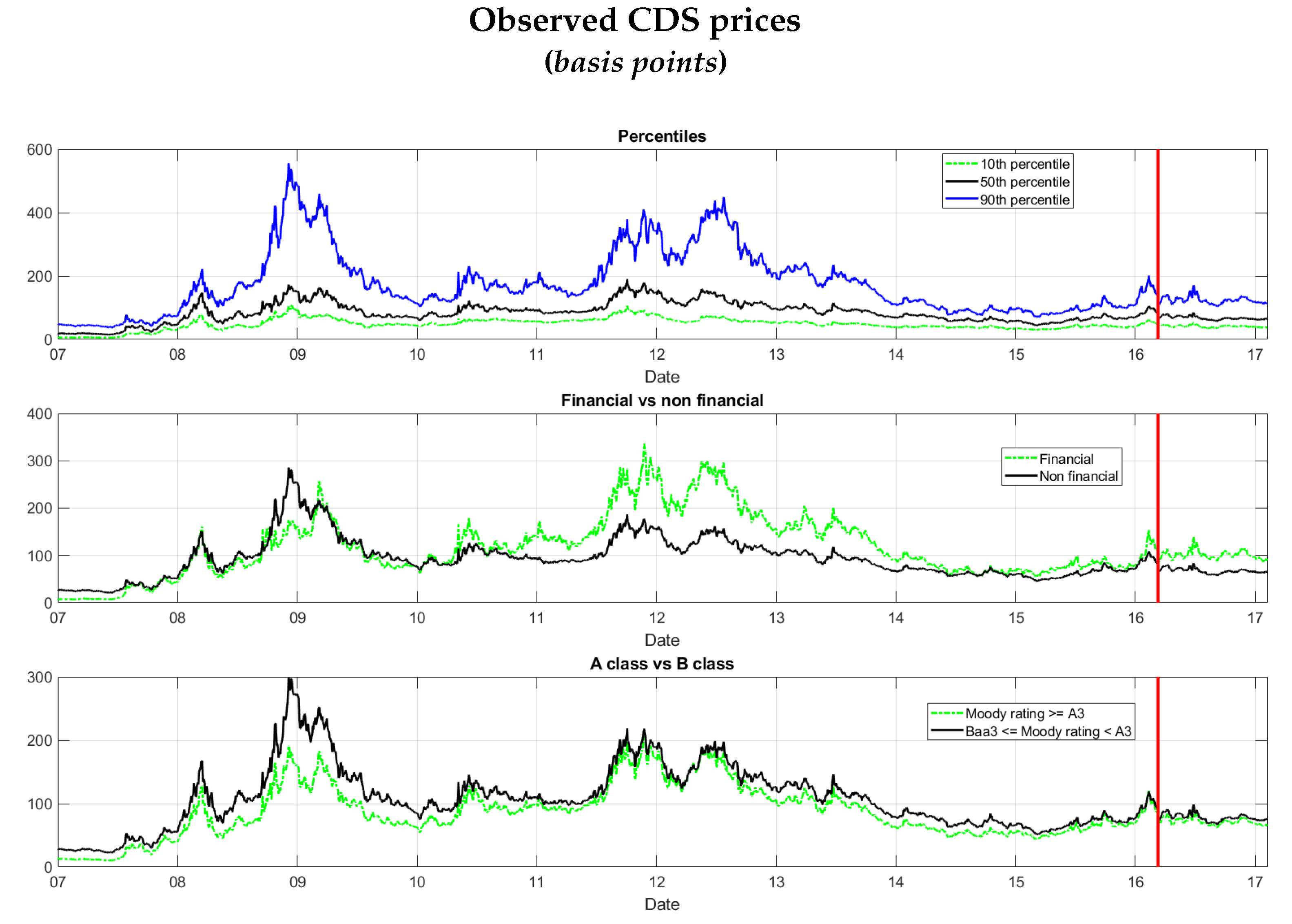
3. Data and Econometric Framework

We use daily time series of closing prices of CDSs with maturities 1 year, 3 years and 5 years, for the firms in the ITraxx Europe Series 26, downloaded from Capital IQ, and for these firms the related EDFs at 1 year, 3 years and 5 years, with source Moody’s KMV. The sample period runs from 1 January 2007 to 6 February 2017.
From the 125 firms of the iTraxx index, in order to have the entire time series dataset for both CDS prices and EDFs, we end up with 102 firms. Among these, we have 25 financial firms and 77 non-financial firms. In terms of credit rating, all are investment grade, but 63 have a Moody’s rating between Baa3 and Baa1 (and we refer to them as being in the B investment grade class), and 39 are classified by Moody’s between A3 and Aaa rating class (and we refer to them as being in the A investment grade class). Given the high variation of CDS prices not only across firms but also over time, instead of reporting static descriptive statistics, we show in Figure 1 the time series of 5-year CDS prices percentiles, as well as the average prices in the two sectors, finacial and non financial, and in the two investment grade rating classes A and B. The same information on 5-year EDFs is reported in Figure 2.
As in Driessen (2005); Diaz et al. (2013) the estimation strategy follows a two-step procedure:
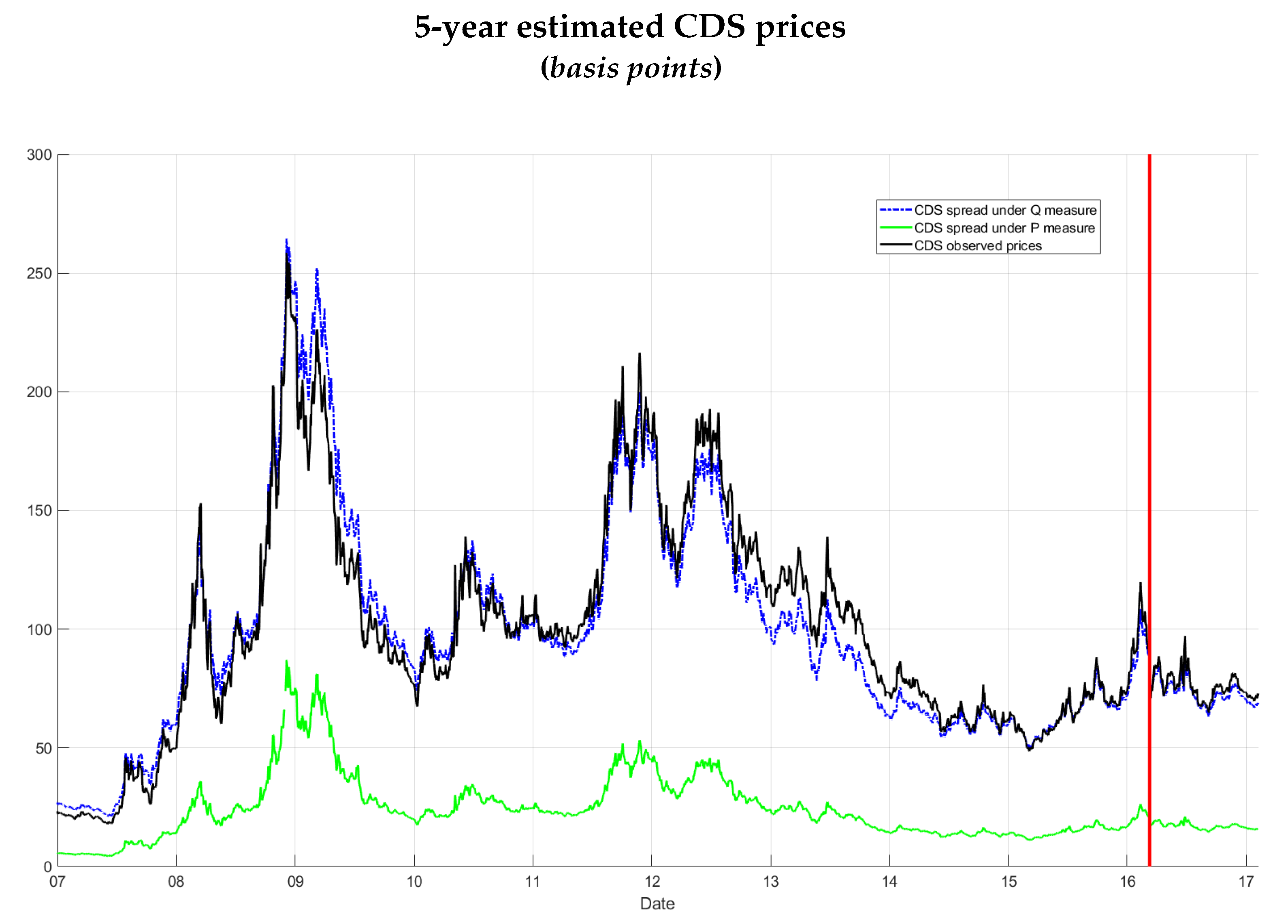
  • We get the maximum likelihood (ML) estimates of the risk-neutral mean of default arrival rates λ t Q from the CDS spreads. Assuming that the default event is diversifiable, we get an estimate of the distress risk premium.
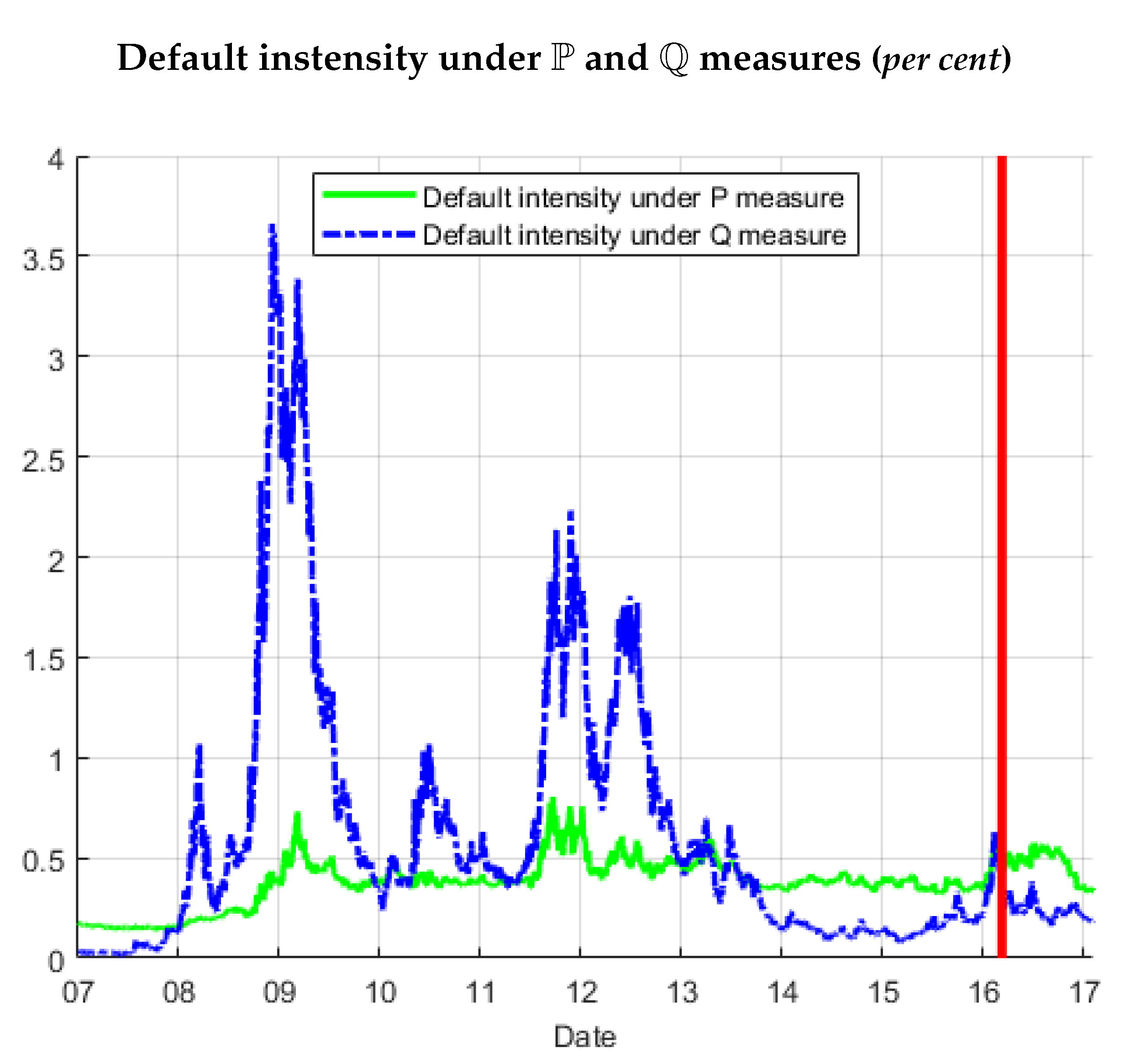
  • We estimate the ML actual default intensity λ t P using information on the actual probabilities of default embedded in Moody’s KMV EDFs.22 We thus compute the jump-at-default risk premium in terms of the ratio λ t Q λ t P , as shown by Driessen (2005); Pan and Singleton (2006).
Our maximum likelihood estimation strategy is based on Chen and Scott (1993),23 and has also been employed in a similar context by Berndt et al. (2005); Pan and Singleton (2008); Longstaff et al. (2011).

3.1. Maximum Likelihood Estimates of Risk-Neutral Default Intensity

Let us first consider the estimates of λ t Q from the CDS spreads.
For each time t, we have one unobservable factor, λ t , and three corresponding CDS prices, with different maturities. Consequently, we must include additional random variables in order to perform a change of variables from unobservable state variables to CDS prices. To this end, we assume CDSs with maturity 3 years ( C D S 3 Y ) as being perfectly priced,24 and we add standard normal measurement errors u 1 Y and u 5 Y for CDSs with maturities 1 and 5 years ( C D S 1 Y and C D S 5 Y ), respectively.
C D S t s Y = f C D S s Y + u t s Y s = 1 , 3 , 5
where
u t 3 Y = 0
ϕ ( u t 1 Y , u t 5 Y ) = 1 ( 2 π ) 2 | Ω | e 1 2 u t Ω 1 u t
and Ω is the diagonal covariance matrix for the measurement errors, with the variances of the measurement errors σ 1 y 2 and σ 5 Y 2 on the diagonal.
To build the maximum likelihood estimator for the parameters of our model, we develop a likelihood function for the observed CDS prices as functions of the unobserved default intensities. It is important to remark that while for CDS prices we consider the dynamics under the risk-neutral measure Q , when we deal with the time series of default intensities, we must use the dynamics under the objective measure P . The vector of parameters that we are going to estimate is thus Θ = ( K Q , θ Q , K P , θ P , σ λ , σ 1 Y , σ 5 Y ) .
We first obtain a possible path of λ t Q by numerically inverting Equation (11).
Given the Ornstein-Uhlenbeck dynamics for ln λ t ,25 the loglikelihood for the sample of observations log L ( λ t , , λ T ) is that one of a Gaussian AR(1) process (see Hamilton 1994, p. 119).26 Given the relationship (14) and the hypothesis of standard normal measurement errors in our model, the log-likelihood function for the entire framework results in the following form:
log L ( λ t , , λ T ) t = 1 T ( log | B t | + log ( 2 π ) + 1 2 log σ 1 y 2 + 1 2 log σ 5 y 2 + ( u t 1 y ) 2 2 σ 2 + ( u t 5 y ) 2 2 σ 2 )
where the elements of the matrix B are such that the Jacobian of the transformation from λ t Q to C D S t is | B t | 1 , and σ 1 y and σ 5 y are the standard deviations of the measurement errors for the CDSs with maturity 1- and 5-years, respectively.

3.2. Maximum Likelihood Estimates of Actual Default Intensity

For the estimates of the objective default intensity λ t P our dataset consists of 1-, 3- and 5-year EDFs from Moody’s KMV. We employ the same methodology as in Section 3.1, of which in the following we briefly recall the main steps. We assume that 3-year EDFs are observed without error. To estimate the parameters of λ t P we maximize the likelihood of the joint density of process (13) and the mispricing errors, related to 1- and 5-year EDFs. To this aim we first get a possible path of λ t P by inverting Equation (12). Mispricing errors of 1- and 5-year EDFs are normally distributed with zero mean and standard deviations σ 1 y and σ 5 y , respectively. To calculate the expectation in Equation (12) for the intensity process (13) we employ as before the finite difference method of Crank-Nicholson.

4. Estimates of the Two Risk Premia Components

In this section we describe the estimation results related to the two sources of excess return.

4.1. Estimation Results of the Distress Risk Premium

Table 1 provides summary statistics of maximum likelihood estimates of the parameters of the risk-neutral process λ t Q .
Looking at these results we can see that, on average, mean-reversion rates are higher under actual than under risk-neutral measure ( K P > K Q ). In contrast, long-term mean parameters are higher under Q than P measure ( θ Q > θ P ). These results are consistent with the empirical evidence in the literature (see, for instance, Pan and Singleton (2008); Diaz et al. (2013) and imply that λ Q will tend to be larger under Q than under P ; in other words the arrival of credit events is more intense in the risk-neutral (higher long-run means) than in the actual environment. Moreover, for a given level of λ Q , there is more persistence under Q than under P (bad times last longer in the risk-neutral world as the speed of mean reversion is lower under Q ).
Remembering the choice of the market price of risk Λ t and the related relatiosnship between the parameters under Q and P measures, we can compute the average market price of risk parameters:
γ 0 = K P θ P K Q θ Q σ λ = 1.1749
and
γ 1 = K Q K P σ λ = 0.0862 .
These parameters determine a negative Λ t , for each t: on average we have
Λ ¯ = γ 0 + γ 1 ln λ Q ¯ = 0.6699 .
We can say that the negative sign of coefficients γ 0 and γ 1 confirm that the credit environment is worst under risk-neutral than under actual measure. According to Pan and Singleton (2008), it is this pessimism about the credit environment that allows risk-neutral pricing to recover market prices in the presence of investors who are averse to default risk.
From the estimates of the parameters of the process λ t Q under both Q and P measures, we can compute the distress risk premium as in Equation (10).
Figure 3 shows the average prices of the 5-year CDSs estimated under the risk-neutral measure Q (blue line) and the objective measure P (green line), and the observed prices (black line). We can see that the fit of risk-neutral prices to observed prices is very good. Risk-neutral prices are consistently higher than the corresponding prices under the objective measure, as they take into account the investors’ risk aversion; moreover the difference between the two time series is greater in periods of financial stress. Let us remark that the line representing CDS prices under the objective measure corresponds to the time series of the estimated expected losses.
Figure 4 shows the estimated average distress risk premia for the firms in the iTraxx index (upper panel), the percentiles of the distress risk premia (second panel), the different behaviour of the distress risk premia for financial and non-financial firms (third panel) and according to rating class (lower panel).
According to the intuition and the empirical evidence in the literature, we can see that the distress risk premium increases considerably during the periods of the financial crisis and the sovereign debt crisis. Furthermore, there is a considerable dispersion among the firms in the index, as we can see by observing the percentiles. It is also clear that while both financial and non-financial firms were deeply affected by the financial crisis, the sovereign debt crisis has hit most financial firms. Finally, as we expect, the distress risk premium of the firms in the lower rating classes is higher than in the higher rating classes.

4.2. Estimation Results of the Jump-at-Default Risk Premium

Table 2 displays the average parameters of the actual default instensity process λ t P :
In Figure 5 we show the average 5-year EDFs reported by Moody’s KMV and estimated with our model, which results in providing a good fit to the data.
Once we estimated the actual default intensities, we can calculate the jump-at-default premium λ t Q / λ t P as well as the market price of jump-at-default risk Γ t . The jump-at-default premium ratio results in approximately 2.9 on (averaged) median for the firms under study. This estimate is consistent with those previously reported in the literature for the US market (see, among others, Driessen (2005)) and for the European market (see for instance Diaz et al. (2013)). Employing the definiton of jump-at-default-risk premium in Equation (1), and having assumed a recovery rate of 40 % , we have
J A D R P t = ( 0.4 1 ) * λ t P * ( 1 λ t Q λ t P )
Figure 6 shows the estimated average jump-at-default risk premia for the firms in the iTraxx index (upper panel), the percentiles of the jump-at-default risk premia (second panel), the different behaviour of the jump-at-default risk premia for financial and non-financial firms (third panel) and according to rating class (lower panel). Our (averaged) median jump-at-default estimate is 11 basis points, that is in line with the existing literature (Diaz et al. (2013) estimate a (averaged) median jump-at-default of 13 basis points). This result indicates that the default event itself entails a risk premium and that this premium increases during the times of stress, which agrees with the intuition on the jump-at-default risk premium. It is evident that the average jump-at-default risk premium is slightly negative in periods of calm. In fact, according to Formula (15), jump at default risk premium is negative if λ P > λ Q , and this happens, on average, during calm periods, as shown in Figure 7.
The jump-at-default-risk-premium is not statistically different from zero during calm periods. Negative values could derive from the problem of the realibility of the estimates λ P , a problem that persists in the existing literature: in fact, the estimate of the actual default intensity is a really difficult task, and we do not count on optimal estimates of it. However, we use the EDFs because they have a higher predictive power than credit ratings, depending on stock prices and being time-variant. Several empirical studies corroborate the accuracy of EDFs for predicting default.27 Additionally, using EDFs to determine the default premium has also been referred to in Berndt et al. (2005) for US corporate CDS spreads, in Vassalou and Xing (2004) for stock prices and in Pan and Singleton (2006) for the CDS spreads of Japanese banks.
The problem of negative jump-at-default risk premium disappears when looking at the median, as we can see in Figure 6.

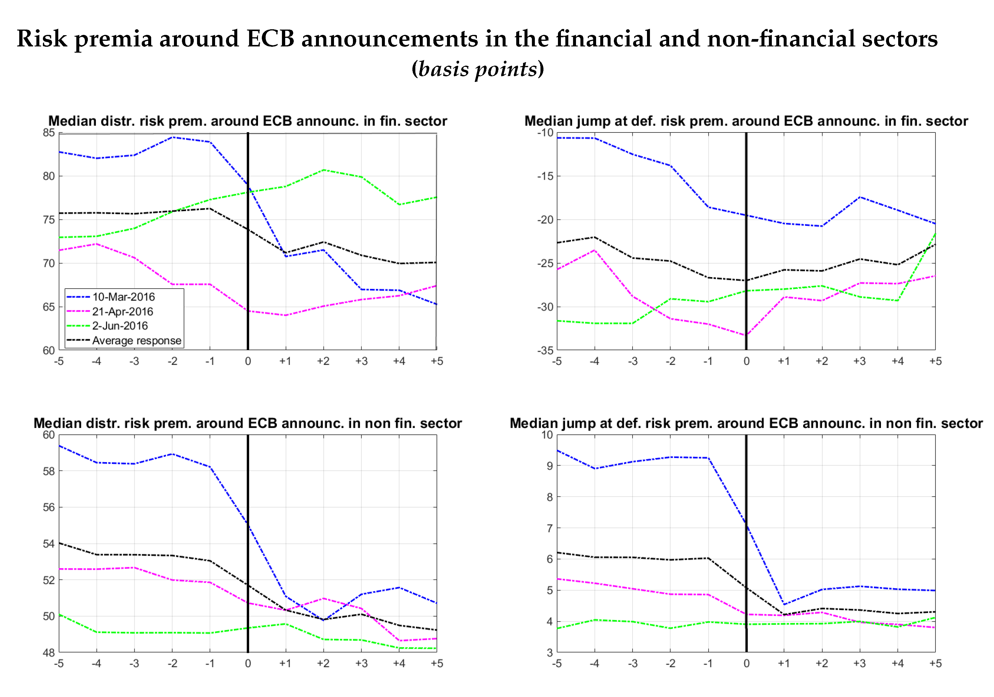
5. Analysis of the Two Risk Premium Components and Event Study Exercise on the Risk Premia and the Expected Losses

By combining the two estimated risk premia, the distress risk premium and the jump-at-default risk premium, we get the excess return of the corporate bond:
e t = D R P t + J A D R P t
Figure 8 shows the time series of the estimated average excess return.
According to our estimates, the (averaged) median distress risk premium in the entire sample period is around 60 basis points and accounts for 88 % of the excess return, while the remaining (averaged) median jump-at-default risk premium is around 11 basis points and accounts for the residual 12 % . If we look at the most recent period, the contribution of the distress risk premium is even higher: in the data sample starting from January 2016 the (averaged) median distress risk premium is around 53 basis points and accounts for 93 % , while the (averaged) median jump-at-default risk premium is around 3 basis points and accounts for 7 % . An interesting comparison is between the behaviour of the two components of the risk premium in the financial and non-financial sectors. Looking at the same recent period, we can say the following:
  • The (averaged) median distress risk premium is higher for financial firms (around 69 basis points, versus 49 basis points of the non financial counterparties);
  • On the contrary, the (averaged) median jump-at-default risk premium is higher for non-financial firms (being around 4 basis points, versus a negative value of the financial counterparties);
  • There is a greater heterogeneity among financial firms compared to non-financial counterparties, as both the dispersion in the distress risk premium and in the jump-at-default risk premium are higher for financial firms: in particular the average standard deviation of the distress risk premium is around 30 basis points for financial firms, compared to 22 for non-financial firms; the average standard deviation of the jump-at-default risk premium is around 73 basis points, compared to 19 for non-financial firms.
We conduct an event study exercise around the key announcements of the ECB relating to the Corporate Sector Purchase Programme (CSPP) during press releases to investigate the effects of these announcements, and thus of the launch of this programme, in the decrease of the two risk premium components. We consider the following dates:28
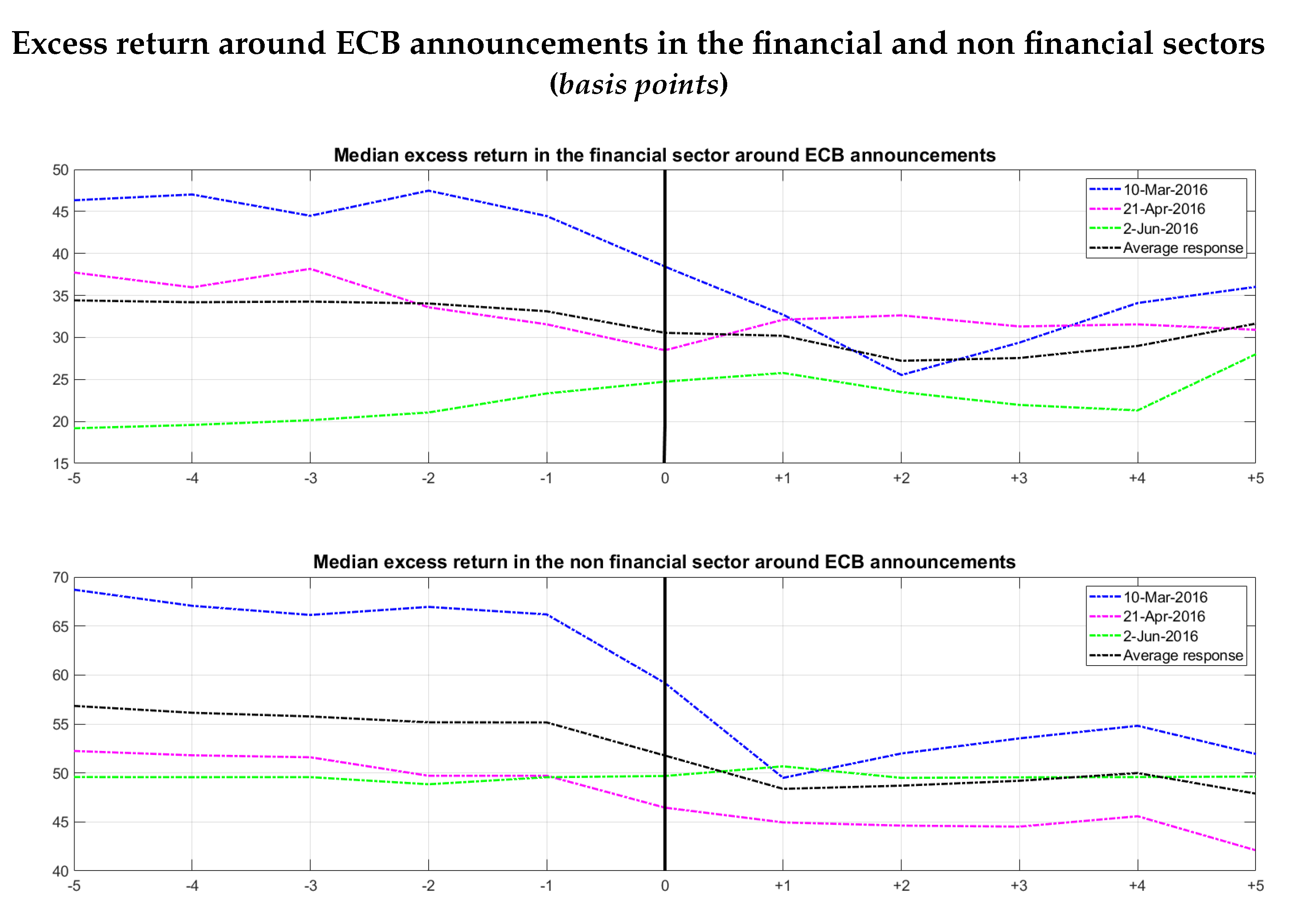
  • 10 March 2016: the ECB adds corporate sector purchase programme (CSPP) to the asset purchase programme (APP);29
  • 21 April 2016: Press Release: the ECB announces details of the corporate sector purchase programme (CSPP), mainly on the eligibility of bonds;30
  • 2 June 2016: the ECB communicates the remaining details of the corporate sector purchase programme (CSPP) on the issuer’s eligibility.31
We use a time window of ten days, five before and five after the announcements. Unfortunately, we cannot use a difference in difference methodology32 to adjust for changes in financial sector risk because also corporate spreads of financial institutions benefited from ECB decisions in those dates. In terms of rating, all the bonds of the firms in the iTraxx are eligible for the purchases in the CSPP, having an investment grade rating.
Figure 9 shows the median of the corporate bond excess return around the dates of the announcements, while Figure 10 shows separately the two components of excess return—the median of the distress risk premium and the median of the jump-at-default risk premium—around the same dates. Looking at these figures it is evident that most of the decrease in both risk premia was observed on 10 March 2016. Indeed, even in ECB Economic Bulletin (2016) is pointed out that "the announcement of the CSPP on 10 March was followed by a significant contraction in the spread between yields on bonds issued by non-financial corporations (NFCs) and a risk-free rate". A further contraction in spreads can be observed on 21 April (when the eligibility of insurance corporations was confirmed), while in June, spreads developments where also related to the uncertainty generated by the referendum in the United Kingdom. Table 3 shows the average variations of the excess return and its components between the day following the announcement of the ECB on 10 March and the previous day, while in Table 4 we can see the historical daily variations. Looking at the different magnitudes of the variations reported in the two tables, we can say that the reductions observed on 10 March where significant.
Table 5 reports the percentage variations of the excess return and its components between the day following the announcement of the ECB on 10 March and the previous day.
Decreases in the distress risk premium and the jump-at-default risk premium were, on average, 15.8 and 34.5 per cent respectively, between the day after this announcement and the previous day. We can therefore state that the jump-at-default component has been more influenced, in relative terms, by the announcement of the CSPP.
With the same event study exercise we can also analyze the different responses of the financial and non-financial sectors to the CSPP announcements.
Figure 11 shows the median of the corporate bond excess return of the financial and non-financial sectors, around the dates of the announcements, while Figure 12 shows separately the two components of the excess return—the median of the distress risk premium and the median of the jump-at-default risk premium in the two sectors—around the same dates.
Table 6 displays the average variations of the excess return and its components, for the financial and non-financial sectors, between the day after the ECB announcement on 10 March and the day before; in Table 7 we can see the related percentage variations.
What is evident is that the spillovers of the launch of the CSPP to the financial sector have been quite important: in relative terms the decline in the excess return of the financial sector was even slightly higher than in the non-financial sector ( 26 % vs. 25 % ), as well as the reduction of the distress risk premium component; the percentage change in the jump-at-default risk premium component was instead more pronounced in the non-financial sector.
To verify that the changes in the estimated components of risk premia after the announcements were substantial, Table 8 shows the daily historical variations of the excess return and its components for the financial and non-financial sectors and we can confirm that they are significantly smaller.
In addition to risk premia, we know that a CDS price incorporates compensation for expected losses. If we also add estimates of expected losses, we obtain the decomposition of the CDS price in its three components. Figure 13 shows on selected dates the average estimates of the expected losses, the distress risk premium and the jump-at-default risk premium.
We can also estimate the effect of the CSPP on the expected losses component of the CDS prices, observing the change in the CDS price under the P measure: on average, between the day before the CSPP announcement and the day later, expected losses decreased by 3.7 basis points; the reduction for financial firms was more pronounced than for non-financial counterparties ( 5.2 versus 3.2 basis points). These variations are quite important, given that the historical daily changes in the expected losses components are on average 0.003 basis points for the entire sample and 0.006 and 0.002 basis points for financial and non-financial firms, respectively.

6. Conclusions

Among the unconventional monetary policy measures recently adopted by the ECB, the Corporate Sector Purchase Program (CSPP) exercised in particular a downward pressure on corporate bond spreads. We contribute to the recent literature on the assessment of the effectiveness of unconventional monetary policy measures, with a focus on the corporate bond market. Corporate bonds are carefully monitored by central banks because they constitute an important channel of transmission of monetary policy decisions to the real economy.
The purpose of this paper is to investigate whether the reduction observed in corporate bond spreads after the launch of the program can be attributed more to a reduction in expected losses or to a reduction in risk premia, and in particular to the compensation requested by investors for the changes in the the credit environment associated with business and macro conditions and the compensation for the risk associated with a jump in the price of the bond in the event of default.
To this end, following Diaz et al. (2013), we use the information embedded in the credit default swaps of the firms in the iTraxx Europe index and the corresponding Expected Default Frequencies to break down the excess return of the corporate bond of each firm into two sources of risk premia: the distress risk premium and the jump-at-default risk premium. Our estimates are in line with those previously reported in the literature. In relative terms, we find that the distress risk premium accounts for approximately 88 % of the total excess return on (averaged) median, historically. On the other hand, the jump-at-default risk premium represents the remaining 12 % on (averaged) median. If we limit our time horizon to the most recent period (from January 2016), the relative contribution of the distress risk premium has even increased, reaching 93 % of the excess return. The risk premia estimated show significant and interesting variations not only over time, with marked increases in both risk premium components during the two main crisis periods of the last ten years (the financial crisis and the sovereign debt crisis), but also among type of firms (although the bonds are all investment grade rated) and sectors. In particular, in the recent period the dispersion of both components of the risk premium is higher for financial firms; in addition, this sector exhibits a higher distress risk premium, while the jump-at-default risk premium is more pronounced for non-financial firms.
Our analysis also allows us to estimate the expected losses component of the CDS price, provided by the CDS price obtained under the objective probability measure (which does not reflect the investors’ risk preferences).
To assess on which source of risk premium the CSPP has been most effective, we perform an event study exercise around the dates of ECB announcements related to the launch of this program and we can see, as we would expect, that the date correspondent to the main drop in the CDS price and its components, is the date of the first announcement of the program, 10 March 2016. Looking at the variations between the day before and the day after the first announcement of the program, we find that on average the reduction in risk premia was around 16.7 basis points ( 10.9 and 5.8 basis points for the distress risk premium and the jump-at-default risk premium, respectively), while the reduction in expected losses was around 3.7 basis points, suggesting a more important effect of the CSPP on the risk premia component, and in particular on the distress risk premium component; however, even the reduction in the expected losses component is not negligible, proving that the CSPP has also contributed to decreasing the default probability of the issuers, improving financial conditions and expectations on the economic outlook. From the same exercise, we also identify important spillovers of the launch of the CSPP to the financial sector, in particular in terms of reducing the distress risk premium and expected losses.
Object of the future research will be an analysis of systemic and idiosyncratic risk in the corporate bond market, based on our firm-by-firm analysis and a comparison of the results obtained by calibrating the model on the overall iTraxx index with those of a theoretical iTraxx index obtained from the aggregation of single CDSs.

Funding

This research received no external funding.

Acknowledgments

I would like to thank Lorenzo Braccini, Francesco Corsello, Davide Delle Monache, Antonio Di Cesare, Stefano Neri, Marcello Pericoli, Pedro Serrano, Marco Taboga and Gabriele Zinna for their helpful comments and suggestions. The views expressed in this paper are those of the author and do not necessarily reflect those of the Bank of Italy. All the remaining errors are my own.

Conflicts of Interest

The authors declare no conflict of interest.

Appendix A

Appendix A.1. Decomposition of the Excess Return into Two Components

In this appendix we provide mathematical evidence to explain the different sources of excess return of a defaultable security. A first approach consists of looking at the equation for the price dynamics under actual and risk-neutral measures.33 The price of a default-risky bond can be considered to depend on a set of state variables X t the follow a diffusion process
d X t = μ X P ( X t , t ) d t + σ X ( X t , t ) d W t P
where μ X P and σ X are the drift and instantaneous volatility, respectively, under the actual measure P . According to Girsanov’s theorem the same equation can be represented under the risk-neutral measure Q :
d X t = μ X Q ( X t , t ) d t + σ X ( X t , t ) d W t Q
where
W t Q = W t P + 0 t Λ t d s ,
and
μ X Q = μ X P ( X t , t ) σ X ( X t , t ) Λ t
are the Brownian motion and the drift under the risk-neutral measure Q , with Λ t being the price of risk.
The dynamics of the price P ( t , X t ) can be represented by applying Ito’s lemma34 under Q measure:
d P ( X t , t ) = P ( X t , t ) t d t + P ( X t , t ) X t r t d t + P ( X t , t ) X t σ X ( X t , t ) d W t Q
+ 1 2 2 P ( X t , t ) X t 2 σ X 2 ( X t , t ) d t + ( R t P ( X t , t ) ) λ t Q d t
and under P measure:
d P ( X t , t ) = P ( X t , t ) t d t + P ( X t , t ) X t ( r t + σ X ( X t , t ) Λ t ) d t + P ( X t , t ) X t σ X ( X t , t ) d W t P
+ 1 2 2 P ( X t , t ) X t 2 σ X 2 ( X t , t ) d t + ( R t P ( X t , t ) ) ( λ t Q ψ ( t ) λ t P ) d t
with ψ ( t ) = λ Q λ P 1 . The expected excess return of the risky-bond can be defined as the difference of expectations under Q and P measures:
E P d p ( X t , t ) P ( X t , t ) E Q d p ( X t , t ) P ( X t , t ) = 1 P t P t X t σ X ( X t , t ) Λ t + P ( X t , t ) R t P ( X t , t ) λ t P ψ t

Appendix A.2. Ito’s Lemma for a Process with Drift, Diffusion and Poisson Jumps

In this appendix we just want to provide the main intuition/ingredients underlying the Ito’s lemma when we have a process that includes jumps.35 Consider a Poisson process with jump intensity λ 1 .36 The probability of a jump in the interval [ t , t + Δ t ] is λ 1 Δ t . The survival probability p ¯ ( t ) (i.e., the probability that no jump has occurred in the interval [ 0 , t ] ) is
p ¯ ( t ) = e 0 t λ 1 ( s ) d s .
Let X ( t ) be a discontinuous stochastic process and denote X ( t ) the value of X as we approach t from the left. Denote by d j X ( t ) the non-infinitesimal change in X(t) as a result of a jump. Then
d j X ( t ) = lim Δ t 0 ( X ( t + Δ t ) X ( t ) ) .
Let z be the magnitude of the jump and let η ( X ( t ) , z ) be the distribution of z. The expected magnitude of the jump is
E [ d j ( X ( t ) ] = λ 1 ( X ( t ) ) d t z z η ( X ( t ) , z ) d z .
Define d J X ( t ) , a compensated process and martingale, as
d J X ( t ) = d j X ( t ) E [ d j X ( t ) ] .
Then
d j X ( t ) = E [ d j X ( t ) ] + d J X ( t ) = λ 1 ( X ( t ) ) z z η ( X ( t ) , z ) d z + d J X ( t ) .
Consider now a function f(X(t), t) of the jump process dX(t). If X(t) jumps by Δ x then f ( X ( t ) ) jumps by Δ f . Δ f is drawn from distribution η f ( ) . The jump part of f is
f ( X ( t ) ) f ( X ( t ) ) = λ 1 ( t ) d t Δ f Δ f η f ( · ) d Δ f + d J f ( t ) .
Let X t be a diffusion process with jumps, defined as the sum of a drift term, a Brownian stochastic integral and a compound Poisson process:
X t = X 0 + 0 t μ s d s + 0 t σ s d W s + i = 1 N t Δ X i .
Then, the process f ( t , X t ) can be represented in differential notation as:
d f ( t , X t ) = f t ( t , X t ) d t + μ t f x ( t , X t ) d t + σ t 2 2 2 f x 2 ( t , X t ) d t
+ f x ( t , X t ) σ t d W t + [ f ( X t + Δ X t ) f ( X t ) ] .
The term linked to the Girsanov transform is related to the derivative term (in addition to the usual derivative in case of a diffusion process) that comes from the change of the intensity of jumps: to change from a Poisson variable N of parameter λ 1 to a variable of parameter λ 2 , the derivative is
d P 2 / d P 1 ( N ) = ( λ 2 / λ 1 ) N exp ( λ 2 λ 1 ) .

Appendix A.3. Ornstein Uhlenbeck Dynamics for the Risk-Neutral Default Intensity under the Objective Probability Measure

Consider the Ornstein Uhlenbeck dynamics for the logarithm of the default intensity λ t under the risk-neutral probability measure Q :
d ln λ t Q = K Q ( θ Q ln λ t Q ) d t + σ λ d W t Q
Assume a market price of risk of the form
Λ t = γ 0 + γ 1 ln λ t
We can write the relationship between the Wiener process under the risk-neutral measure W t Q and the Wiener process under the objective measure W t P as
W t Q = W t P + 0 t γ 0 + γ 1 ln λ s d s
and, in differential terms,
d W t Q = d W t P + ( γ 0 + γ 1 ln λ t ) d t .
We can therefore express (A10) in terms of W t Q as
d λ t = ( K Q θ Q + σ γ 0 ( K Q σ γ 1 ) ln λ t ) d t + σ λ d W t P = K P ( θ P ln λ t ) d t + σ λ d W t P
where
K P θ P = K Q θ Q + σ λ γ 0 ;
K P = K Q σ λ γ 1 .

Appendix A.4. CIR Dynamics for the Risk-Neutral Default Intensity under the Objective Measure

Consider the CIR dynamics for the default intensity λ t under the risk-neutral measure Q :
d λ t = K Q ( θ Q λ t ) d t + σ λ λ t d W t Q
K Q is the speed of adjustment, and must be strictly positive; to assure a λ t Q strictly positive we must also impose the Feller condition: 2 K Q θ Q > σ λ 2 .
We assume a market price of risk as in Cheridito et al. (2007)
Λ t = γ 0 λ t + γ 1 λ t
We can write the relationship between the Wiener process under the risk-neutral measure W t Q and the Wiener process under the objective measure W t P as
W t Q = W t P + 0 t γ 0 λ s + γ 1 λ s d s
and, in differential terms,
d W t Q = d W t P + γ 0 λ t d t + γ 1 λ t d t .
We can therefore express (A12) in terms of W t Q as
d λ t = K Q θ Q + σ γ 0 ( K Q σ γ 1 ) λ t d t + σ λ λ t d W t P = K P ( θ P λ t ) d t + σ λ λ t d W t P
where
K P θ P = K Q θ Q + σ λ γ 0 ;
K P = K Q σ λ γ 1 .
To satisfy the Novikov condition we must impose γ 0 K 0 P θ P 1 2 .

Appendix A.5. Explicit Solution for the CDS Price in the CIR Model

Under the risk-neutral measure Q consider the equation for the CDS price
C D S t Q ( M ) = ( 1 R Q ) t t + M D ( t , u ) E t Q λ u Q e t u λ s Q d s d u t t + M D ( t , u ) E t Q e t u λ s Q d s d u
and the CIR dynamics for λ t Q as in (9)
We can explicitly solve the two expectations in (A14)37 as
E t Q λ u Q e t u λ s Q d s = K Q θ Q A ( u t ) + A ( u t ) u λ t Q · C ( u t ) e A ( u t ) λ t Q
E t Q e t u λ s Q d s = C ( u t ) e A ( u t ) λ t Q
where
A ( u t ) = 2 ( e γ ( u t ) 1 ) ( γ + K Q ) ( e γ ( u t ) 1 ) + 2 γ
A ( u t ) u : = B ( u t ) = 4 γ 2 e γ ( u t ) ( ( γ + K Q ) ( e γ ( u t ) 1 ) + 2 γ ) 2
C ( u t ) = 2 γ e 1 2 ( γ + K Q ) ( u t ) ( γ + K Q ) ( e γ ( u t ) 1 ) + 2 γ 2 K Q θ Q σ λ 2
and
γ = K Q 2 + 2 σ λ 2 .

Appendix A.6. PDE Associated with the Expectation and Crank Nicholson Scheme

Consider a stochastic process
d y t = p ( y , t ) d t + σ ( y , t ) d W t
with W t standard Brownian motion, and the partial differential equation
S t + S y p ( y , t ) + 1 2 S y y σ ( y , t ) 2 = c ( y , t ) S
with boundary condition g ( y , T ) at T, where p ( y , t ) and c ( y , t ) are two functions of y and t. According to the Feynman–Kac theorem, the solution of Equation (A15) is given by
S ( y , T ) = E Q [ e t T c ( y u , u ) d u g ( y T , T ) ] .
In our paper we want to compute E Q [ e t u λ s d s ] so we set
y t : = x t = ln λ t
p ( y , t ) : = K θ K x t
σ ( y , t ) : = σ
c ( y u , u ) : = λ s = e x s
g ( y T , T ) : = 1 .
Our expectation is then solution of the following PDE:
S t + S x ( K θ K x t ) + 1 2 S x x σ 2 = e x t S
with boundary condition S ( x , u ) = 1 .
At this point we can employ the Crank-Nicholson scheme to solve it. This is a finite difference method that consists of replacing terms in Equation (A15) by approximation in discrete time and space. Consider: N time steps with t i t i 1 = Δ t constant; L space steps with x j x j 1 = Δ x constant. We can approximate the derivatives in time and space as
S t S j , i + 1 S j , i Δ t
S x 1 2 S j + 1 , i S j 1 , i 2 Δ x + 1 2 S j + 1 , i + 1 S j 1 , i + 1 2 Δ x
2 S x 2 1 2 S j + 1 , i 2 S j , i + S j 1 , i Δ x 2 + 1 2 S j + 1 , i + 1 2 S j , i + 1 + S j 1 , i + 1 Δ x 2
S S j , i + S j , i + 1 2 .
Using these aproximations we can rewrite Equation (A17) as
S j , i + 1 S j , i Δ t + ( K θ + K X t ) S j + 1 , i S j 1 , i + S j + 1 , i + 1 S j 1 , i + 1 4 Δ x + 1 2 S j + 1 , i 2 S j , i + S j 1 , i + S j + 1 , i + 1 2 S j , i + 1 + S j 1 , i + 1 2 Δ x 2 σ 2 = e X t S j , i + S j , i + 1 2 .
After some simple algebra calculations Equation (A18) becomes
A i S j + 1 , i + 1 + B i S j , i + 1 + C i S j 1 , i + 1 = A i S j + 1 , i D i S j , i C i S j 1 , i ,
that can be written in matrix form as
M 2 S i + 1 = M 1 S i
where S i = [ S 1 , i , S 2 , i , , S L 1 , i ] T ,
M 1 = D 1 C 1 A 2 D 2 C 2 A 3 D 3 C 3 A M 2 D M 2 C M 2 A M 1 B M 1
and
M 2 = B 1 C 1 A 2 B 2 C 2 A 3 B 3 C 3 A M 2 B M 2 C M 2 A M 1 B M 1

Appendix A.7. Price of Jump-at-Default Risk

Consider that the jumps in price occure from time to time: the first jump occurs at time τ 1 , the second occurs τ 2 time units after the first, the third occurs τ 3 units after the second, etc. The variables τ 1 , τ 2 , τ 3 . are independent exponential random variables, all with the same mean 1 λ . Because the expected time between jumps is 1 λ , the jumps are arriving at an average rate of λ per unit time. The process N t counts the number of jumps that occur at or before time t, and we say that has intensity λ .
Suppose that under the probability measure P the Poisson process N t has intensity λ t P , and thus distribution:
P ( N t = k ) = ( λ P t ) k k ! e λ P t
We have that the compensated process M t : = N t λ t P is a martingale; if the intensity is time varying, the process N t 0 t λ s P is a P -martingale. Just as we can use Girsanov’s Theorem to change the measure so that a Brownian motion with drift becomes a Brownian motion without drift, and in terms of this change of measure we define the market price of risk, we can change the measure for a Poisson process and define the related jump price of risk. For a Poisson process, the change of measure affects the intensity. We want to change to a measure Q such that N t ( 0 t T ) is a Poisson process with intensity λ t Q , that means that
P ( N t = k ) = ( λ Q t ) k k ! e λ Q t
and the process N t 0 t λ s Q is a Q -martingale. Let us fix the time T > 0 . The Radon-Nykodim derivative that allows the change of measure is the function
Z ( T ) = e ( λ P λ Q ) T λ Q λ P N T
and
Q ( A ) = A Z ( T ) d P
In fact it can be proved38 that the process Z ( t ) satisfies
d Z ( t ) = λ Q λ P λ P Z ( t ) d M ( t ) ,
is a martingale under P and E Z ( t ) = 1 for all t, that is necessary to be able to change the measure.
The jump price of risk can thus be defined as
Γ t Q = λ t Q λ t P 1 or Γ t P = 1 λ t Q λ t P .

References

  1. Berndt, Antje, Rohan Douglas, Darrell Duffie, Mark Ferguson, and David Schranz. 2005. Measuring Default Risk Premia from Default Swap Rates and EDFs. Working Paper No. 173. Basel: BIS, March. [Google Scholar]
  2. Berndt, Antje, and Iulian Obreja. 2010. Decomposing European CDS returns. Review of Finance 14: 189–233. [Google Scholar] [CrossRef] [Green Version]
  3. Bharath, Sreedhar T., and Tyler Shumway. 2008. Forecasting Default with the Merton Distance to Default Model. The Review of Financial Studies 21: 1339–69. [Google Scholar] [CrossRef]
  4. Blanco, Roberto, Simon Brennan, and Ian W. Marsh. 2005. An empirical analysis of the dynamic relation between investment-grade bonds and credit defualt swaps. The Journal of Finance 60: 2255–81. [Google Scholar] [CrossRef]
  5. Cecchetti, Sara, and Marco Taboga. 2017. Assessing the Risks of Asset Overvaluation: Models and Challenges. Working Papers, No. 1114. Rome: Bank of Italy Temi di Discussione, April. [Google Scholar]
  6. Chen, Ren-Raw, and Louis Scott. 1993. Maximum likelihood estimation for a multifactor equilibrium model of the term structure of interest rates. The Journal of Fixed Income 3: 14–31. [Google Scholar] [CrossRef]
  7. Cheridito, Patrick, Damir Filipović, and Robert L. Kimmel. 2007. Market price of risk specifications for affine models: Theory and evidence. Journal of Financial Economics 83: 123–70. [Google Scholar] [CrossRef]
  8. Cox, John C., Jonathan E. Ingersoll Jr., and Stephen A. Ross. 1985. A Theory of the Term Structure of Interest Rates. Econometrica 53: 385–407. [Google Scholar] [CrossRef]
  9. Cont, Rama, and Peter Tankov. 2004. Financial Modelling with Jump Processes. Financial Mathematics Series; Boca Raton: Chapman and Hall/CRC. [Google Scholar]
  10. Diaz, Antonio, Jonatan Groba, and Pedro Serrano. 2013. What drives corporate default risk premia? Evidence from the CDS market. Journal of International Money and Finance 37: 529–63. [Google Scholar] [CrossRef] [Green Version]
  11. Driessen, Joost. 2005. Is Default Event Risk Priced in Corporate Bonds? The Review of Financial Studies 18: 165–95. [Google Scholar] [CrossRef]
  12. Duffee, Gregory R. 2002. Term Premia and Interest Rate Forecasts in Affine Models. Journal of Finance 57: 405–43. [Google Scholar] [CrossRef]
  13. Duffie, Darrell, and Kenneth J. Singleton. 1999. Modeling Term Structures of Defaultable Bond Yields. The Review of Financial Studies 12: 687–720. [Google Scholar] [CrossRef] [Green Version]
  14. Duffie, Darrell, and Kenneth J. Singleton. 2003. Credit Risk: Pricing, Measurement and Management. Princeton: Princeton Series in Finance. [Google Scholar]
  15. European Central Bank. 2016. ECB Economic Bulletin. Issue 5/2016, Box 2. Available online: https://www.ecb.europa.eu/pub/pdf/ecbu/eb201605.en.pdf (accessed on 4 August 2016).
  16. Forte, Santiago, and Pena Juan Ignacio. 2009. Credit spreads: An empirical analysis on the informational content of stocks, bonds, and CDS. Journal of Banking & Finance 33: 2013–25. [Google Scholar]
  17. Gilchrist, S., and Zakrajsek Egon. 2012. Credit Spreads and Business Cycle Fluctuations. The American Economic Review 102: 1692–720. [Google Scholar] [CrossRef]
  18. Hamilton, James D. 1994. Time Series Analysis. Princeton: Princeton University Press. [Google Scholar]
  19. Hamilton, James D., and Wu Jing Cynthia. 2012. Identification and Estimation of Gaussian Affine Term Structure Models. Journal of Econometrics 168: 315–31. [Google Scholar] [CrossRef] [Green Version]
  20. Ishii, Hokuto. 2019. Forecasting Term Structure of Interest Rates in Japan. International Journal of Financial Studies 7: 39. [Google Scholar] [CrossRef] [Green Version]
  21. Jarrow, Robert A., David Lando, and Fan Yu. 2005. Default risk and diversification: Theory and empirical implications. Mathematical Finance 15: 1–26. [Google Scholar] [CrossRef]
  22. Kealhofer, Stephan. 2003. Quantifying credit risk I: Default prediction. Financial Analyst Journal 59: 30–44. [Google Scholar] [CrossRef]
  23. Kelly, Bryan, Hanno Lustig, and Stijn Van Nieuwerburgh. 2016. Too-Systemic-To-Fail: What Option Markets Imply About Sector-wide Government Guarantees. American Economic Review 106: 1278–319. [Google Scholar] [CrossRef] [Green Version]
  24. Korablev, Irina, and Douglas Dwyer. 2007. Power and Level Validation of Moody’s KMV EDFTM Credit Measures in North America, Europe and Asia. Moody’s KMV Technical Report 070930. New York: Moody’s KMV Company, pp. 17–18. [Google Scholar]
  25. Lando, David. 1998. On Cox Processes and Credit Risky Securities. Review of Derivative Research 2: 99–120. [Google Scholar] [CrossRef]
  26. Lando, David. 2004. Credit Risk Modeling. Princeton: Princeton Series in Finance. [Google Scholar]
  27. Li, Junye, and Gabriele Zinna. 2015. On Bank Credit Risk: Systemic or Bank-Specific? Evidence from the US and UK. Journal of Financial and Quantitative Analysis 49: 1403–42. [Google Scholar] [CrossRef]
  28. Longstaff, Francis A., Sanjay Mithal, and Eric Neis. 2005. Corporate yields spreads: Default risk or liquidity? New evidence from the the credit default swap market. The Journal of Finance 60: 2213–53. [Google Scholar] [CrossRef] [Green Version]
  29. Longstaff, Francis A., Jun Pan, Lasse H. Pedersen, and Kenneth J. Singleton. 2011. How Sovereign is Sovereign Credit Risk? American Economic Journal: Macroeconomics 3: 75–103. [Google Scholar] [CrossRef] [Green Version]
  30. Merton, Robert C. 1974. On the pricing of corporate debt: The risk structure of interest rates. The Journal of Finance 29: 449–70. [Google Scholar]
  31. Pan, Jun, and Kenneth J. Singleton. 2006. Interpreting Recent Changes in the Credit Spreads of Japanese Banks. Tokyo: Monetary and Economic Studies, Institute for Monetary and Economic Studies, Bank of Japan, vol. 24, pp. 129–41. [Google Scholar]
  32. Pan, Jun, and Kenneth J. Singleton. 2008. Default and recovery implicit in the term structure of sovereign CDS spread. The Journal of Finance 63: 2345–84. [Google Scholar] [CrossRef] [Green Version]
  33. Schonbucher, Philipp J. 2003. Credit Derivatives Pricing Models. Hoboken: Wiley Finance Series. [Google Scholar]
  34. Shreve, Steven E. 2008. Stochastic Calculus for Finance II. Continuous-Time Models. New York: Springer. [Google Scholar]
  35. Vassalou, Maria, and Yuhang Xing. 2004. Default risk in equity returns. The Journal of Finance 59: 831–68. [Google Scholar] [CrossRef]
  36. Vasicek, Oldrich. 1977. An equilibrium characterization of the term structure. Journal of Financial Economics 5: 177–88. [Google Scholar] [CrossRef]
  37. Yu, Fan. 2002. Modeling Expected Return on Defaultable Bonds. Journal of Fixed Income 12: 69–81. [Google Scholar] [CrossRef]
1.
For a discussion of the decomposition of corporate bond spreads in the expected losses and the risk premium components see, for example, Cecchetti and Taboga (2017).
2.
In Berndt and Obreja (2010) the payments of a CDS can be reproduced by a replicating portfolio consisting of a long position in a defaultable bond and a short position in a risk-free bond.
3.
4.
Meaning that price variations of CDSs anticipate variations in bond spreads. This evidence is consistent with the standard hypothesis whereby CDS prices adjust more rapidly to the release of new information and that adjustment, in turn, generates an informative signal to which bond spreads react with a time lag.
5.
The same decomposition is employed by Pan and Singleton (2006) for the credit spreads of Japanese banks.
6.
As in Pan and Singleton (2008) for sovereign CDS spreads.
7.
This credit-risk literature can be related to the term structure of interest rate models where intuitively, survival probabilities take similar expressions to bond prices, with the default intensity replacing the short rate; in other words, risk-neutral (objective) bond prices relate to risk-neutral (objective) survival probabilities. A seminal paper in the literature of the term structure of interest rates is Vasicek (1977); recently Ishii (2019) examines and compares different models to forecast the term structure of interest rates.
8.
For the dynamics of λ Q , we also studied a different model (starting from Li and Zinna (2015); Cheridito et al. (2007)) from the one used in those papers, but we found that this new model did not perform as well as the first: for this reason we continued our analysis using the consolidated model.
9.
In the CSPP the object of the purchases are the investment grade bonds with residual life between 1 and 30 years, issued by non-financial firms or non-banking financial firms. The purchases can be made both in the primary and the secondary markets.
10.
A completely different approach that also analysis the excess bond premium is in Gilchrist and Zakrajsek (2012).
11.
Discounting by r t + λ t Q captures the survival-dependent nature of the payments.
12.
These strong technical assumptions are standard in the litarature, and necessary to construct the discrete approximation for the solution of the CDS price introduced in Lando (2004), which we’ll see in Section 2.2.
13.
See the Introduction for references and a brief explanation.
14.
Technical proof can be found in Appendix A.3.
15.
16.
According to the authors, the motivation for this choice is to avoid to impose the Feller condition required by the CIR dynamcis to assure a λ t Q strictly positive: 2 K Q θ Q > σ λ 2 . Such choice of market price of risk determines only one different parameter in the processes under the actual and the risk-neutral measure.
17.
Technical proof can be found in Appendix A.4.
18.
See Appendix A.6 for details of this method.
19.
See Yu (2002) for a heuristic discussion.
20.
See Appendix A.7 for a technical explanation.
21.
Empirical studies corroborate the accuracy of EDFs for predicting default (see Kealhofer (2003); Bharath and Shumway (2008); Korablev and Dwyer (2007)) and using EDFs to determine the default premium has been also referred to in Berndt et al. (2005) for US corporate CDS spreads, Vassalou and Xing (2004) for stock prices and Pan and Singleton (2006) for CDS spreads of Japanese banks.
22.
Which are based on the Merton model for picing corporate debt (see Merton (1974)).
23.
See also Hamilton and Wu (2012) for a description of the method.
24.
The same hypothesis is in Longstaff et al. (2011); Diaz et al. (2013), but is not related to different liquidity consitions of CDS contracts with different maturities.
25.
We can consider this dynamics as the continuous time version of the corresponding AR(1) process, or
lim Δ t 0 ln λ t ln λ t 1 = θ ( 1 e K ) + ( e K 1 ) ln λ t 1 + ϵ t ,
with ϵ t N ( 0 , σ ϵ ) and σ ϵ 2 = σ 2 2 K ( 1 e 2 K ) .
26.
A non-central χ 2 distribution, defined in terms of the modified Bessel function of first kind, is instead involved in case of a CIR dynamics for λ t (see Chen and Scott (1993)).
27.
28.
Of course we expect that the main impact on the components of CDS prices arises at the date of the first announcement of the CSPP (as in fact is confirmed by the results), but we also consider the dates of the other two press releases in wich the ECB provides details of the programme.
29.
30.
31.
32.
As often employed in the literature for event study exercises, see for instance Kelly et al. (2016).
33.
Technical details can be also found in Cont and Tankov (2004).
34.
Terms come from Ito’s lemma for a process with drift, diffusion and Poisson jumps (due to default) and Girsanov’s theorem; see Appendix A.2 for a brief overview and Cont and Tankov (2004) for details.
35.
Technical details can be found in Cont and Tankov (2004).
36.
λ 1 could be a constant, a deterministic function of time, or a stochastic process.
37.
Technical details can be found in Duffie and Singleton (2003); Schonbucher (2003).
38.
See Shreve (2008) for technical details.
Figure 1. Time series statistics of 5-year observed CDS prices. The figure shows the time series of the observed 5-year CDS prices of 102 firms selected in the iTraxx index; these prices are displayed in the three panels as percentiles, averages of financial and non financial firms, and averages of A and B investment grade class, respectively. Data are in basis points. The sample period runs from 1 January 2007 to 6 February 2017. The red vertical bar coincides with the date of the first announcement of the ECB related to the CSPP, on 10 March 2016.
Jrfm 13 00003 g001
Figure 2. Time series statistics of Moody’s 5-year expected default frequencies. The figure shows the time series of the Moody’s KMV 5-year expected default frequencies; these data are displayed in the three panels as percentiles, averages of financial and non financial firms, and averages of A and B investment grade class, respectively. Data are in percentages. The sample period runs from 1 January 2007 to 6 February 2017. The red vertical bar coincides with the date of the first announcement of the ECB related to the CSPP, on 10 March 2016.
Jrfm 13 00003 g002
Figure 3. Average 5-year CDS prices observed and estimated under the two probability measures. The figure shows the time series of the average of 5-year CDS prices of 102 firms selected in the ITraxx index. The black line is related to the prices observed in the market, while the blue and the green lines display the averages of the model estimates under the risk-neutral Q and the objective P measures, respectively. Data are in basis points. The sample period runs from 1 January 2007 to 6 February 2017. The red vertical bar coincides with the date of the first announcement of the ECB related to the CSPP, on 10 March 2016.
Jrfm 13 00003 g003
Figure 4. Distress risk premium: average, percentiles and for different classes of firms. The figure shows the time series of the estimated average distress risk premia for the firms in the iTraxx index (upper panel), the percentiles of the distress risk premia (second panel), the averages of distress risk premia in the financial and non-financial subsets (third panel) and in two rating classes subsets (lower panel). Data are in basis points. The sample period runs from 1 January 2007 to 6 February 2017. The red vertical bar coincides with the date of the first announcement of the ECB related to the CSPP, on 10 March 2016.
Jrfm 13 00003 g004
Figure 5. Average 5-year EDFs of source Moody’s and estimated. The figure shows the time series of the average of the 5-year EDFs of source Moody’s KMV (black line) and estimated (green line). Data are in percentages. The sample period runs from 1 January 2007 to 6 February 2017. The red vertical bar coincides with the date of the first announcement of the ECB related to the CSPP, on 10 March 2016.
Jrfm 13 00003 g005
Figure 6. Jump-at-default risk premium: average, percentiles and for different classes of firms. The figure shows the time series of the estimated jump-at-default risk premium; the upper panel displays the average for the firms, the second panel shows the percentiles, the third panel shows the averages for the financial and non-financial subsets, the lower panel shows the averages in two subsets of different rating class. Data are in basis points. The sample period runs from 1 January 2007 to 6 February 2017. The red vertical bar coincides with the date of the first announcement of the ECB related to the CSPP, on 10 March 2016.
Jrfm 13 00003 g006
Figure 7. Average physical and risk-neutral default intensity. The figure shows the time series of the average of the default intensities estimated under the objective P (green line) and the risk-neutral Q (blue line) measures. Data are in percentages. The sample period runs from 1 January 2007 to 6 February 2017. The red vertical bar coincides with the date of the first announcement of the ECB related to the CSPP, on 10 March 2016.
Jrfm 13 00003 g007
Figure 8. Average excess return. The figure shows the time series of the average excess return, obtained as the sum of the estimated distress risk premium and jump-at-default risk premium. Data are in basis points. The sample period runs from 1 January 2007 to 6 February 2017. The red vertical bar coincides with the date of the first announcement of the ECB related to the CSPP, on 10 March 2016.
Jrfm 13 00003 g008
Figure 9. Event study: median of the excess return. The figure shows the median of the estimated corporate bond excess return around key ECB announcements dates (five days before and five days after the announcement date). The black line shows the average risk premium response over all announcements, and the coloured lines show the responses to each individual announcement.
Jrfm 13 00003 g009
Figure 10. Event study: median of the distress and jump-at-default risk premia. The figure shows the median of the estimated distress risk premium and the jump-at-default risk premium around key ECB announcements dates (five days before and five days after the announcement date). In each figure, the black line shows the average risk premium response over all announcements, and the coloured lines show the responses to each individual announcement. Data are in basis points.
Jrfm 13 00003 g010
Figure 11. Event study: median of the excess return in the financial and non financial sectors. The figures show the median of the estimated corporate bond excess return around key ECB announcements dates in the financial and non financial sectors (five days before and five days after the announcement date). In each figure the black line shows the average risk premium response over all announcements, and the coloured lines show the responses to each individual announcement. Data are in basis points.
Jrfm 13 00003 g011
Figure 12. Event study: median of the distress and jump-at-default risk premia in the financial and non-financial sectors. The figures show the median of the estimated distress risk premium and jump-at-default risk premium around key ECB announcements dates (five days before and five days after the announcement date). In each figure, the black line shows the average risk premium response over all announcements, and the coloured lines show the responses to each individual announcement. Data are in basis points.
Jrfm 13 00003 g012
Figure 13. Components of average CDS price. The figure shows the three components of the average CDS price (the average expected losses, the average distress risk premium and the average jump-at-default risk premium) at selected dates: before the financial crisis (January 2007), at the peaks of the financial crisis (January 2009) and of the sovereign debt crisis (January 2012); before the announcement of the programme (March 2016); when the purchases begin (June 2016); at the most recent date (February 2017). Data are in basis points.
Jrfm 13 00003 g013
Table 1. Parameters of risk-neutral default intensity process under risk-neutral and objective probability measures. Summary statistics of maximum likelihood estimates of risk-neutral λ t Q process. K Q and K P denote the mean-reversion rates of λ t Q under the risk-neutral and actual measures, respectively. θ Q and θ P are the long-run mean of λ t Q under the risk-neutral and actual measures, respectively. σ λ is the instantaneous volatility of the process. σ 1 y and σ 5 y represent the volatility of the mispricing errors for 1- and 5-year maturities.
K Q θ Q σ λ K P θ P σ 1 y σ 5 y
Mean0.3288−4.53331.19080.4314−6.66360.00160.0013
Std0.03390.47050.06770.00470.07170.00160.0007
Median0.3294−4.50361.20000.4304−6.67990.00120.0012
Table 2. Parameters of objective default intensity process. Summary statistics of maximum likelihood estimates of actual λ t P process. K P denotes the mean-reversion rate of λ t P under the actual measure. θ P is the long-run mean of λ t P under the actual measure. σ λ is the instantaneous volatility of the process. σ 1 y and σ 5 y represent the volatility of the errors in the EDFs for 1- and 5-year maturities.
α P β P σ λ σ 1 y σ 5 y
Mean0.3035−12.54421.13600.00240.0012
Std.0.094812.63190.17210.00460.0016
Median0.3079−9.39971.17350.00110.0006
Table 3. Average variations around ECB announcements. This table shows the average variations between the day after the ECB announcement on 10 March 2016 and the day before, of the excess return, the distress risk premium and the jump-at-default risk premium. Basis points.
Δ ExRet ¯ Δ DRP ¯ Δ JADRP ¯
−16.75−10.87−5.88
Table 4. Historical daily variations. This table shows the historical daily variations of the excess return, the distress risk premium and the jump-at-default risk premium. Basis points.
h Δ ExRet ¯ h Δ DRP ¯ h Δ JADRP ¯
0.0100.0090.001
Table 5. Average relative variations around ECB announcements. This table shows the average relative variations between the day after the ECB announcement on 10 March 2016 and the day before, of the excess return, the distress risk premium and the jump-at-default risk premium. Percentages.
( Δ ExRet ) / ExRet t 1 ¯ ( Δ DRP ) / DRP t 1 ¯ ( Δ JADRP ) / JADRP t 1 ¯
−21.41−15.84−34.47
Table 6. Average variations around ECB announcements in the financial and non financial sectors. This table shows the average absolute variations between the day after the ECB announcement on 10 March 2016 and the day before, of the excess return, the distress risk premium and the jump-at-default risk premium in the financial and non financial sectors. Basis points.
Δ ExRet f ¯ Δ DRP f ¯ Δ JADRP f ¯ Δ ExRet nf ¯ Δ DRP nf ¯ Δ JADRP nf ¯
−11.75−13.14−1.87−16.68−7.12−4.71
Table 7. Average relative variations around ECB announcements in the financial and non financial sectors. This table shows the average relative variations between the day after the ECB announcement on 10 March 2016 and the day before, of the excess return, the distress risk premium and the jump-at-default risk premium in the financial and non financial sectors. Percentages.
Δ ExRet f ExRet f t 1 ¯ Δ DRP f DRP f t 1 ¯ Δ JADRP f JADRP f t 1 ¯ Δ ExRet nf ExRet nf t 1 ¯ Δ DRP nf DRP nf t 1 ¯ Δ JADRP nf JADRP nf t 1 ¯
−26.43−15.67−10.06−25.20−12.24−50.92
Table 8. Historical daily variations in the financial and non financial sectors. This table shows the average historical daily variations of the excess return, the distress risk premium and the jump-at-default risk premium in the financial and non financial sectors. Basis points.
h Δ ExRet f ¯ h Δ DRP f ¯ h Δ JADRP f ¯ h Δ ExRet nf ¯ h Δ DRP nf ¯ h Δ JADRP nf ¯
0.0170.019−0.0020.0070.0050.002

