Splitting Credit Risk into Systemic, Sectorial and Idiosyncratic Components


Abstract
:1. Introduction
2. Literature Review
3. A Historical Examination of Sectorial CDS Data
3.1. The Data
3.2. Sectorial CDS Indices
3.2.1. Main Statistics
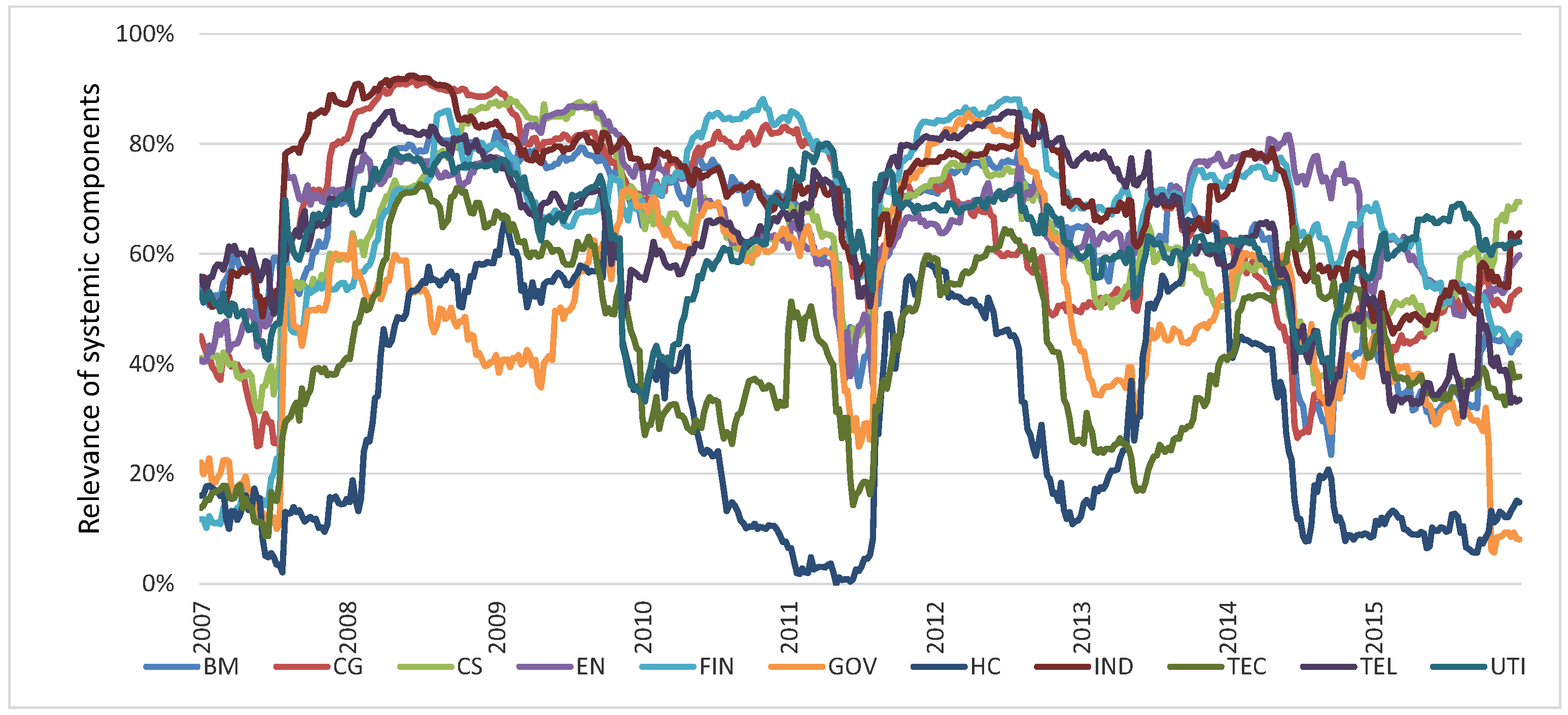
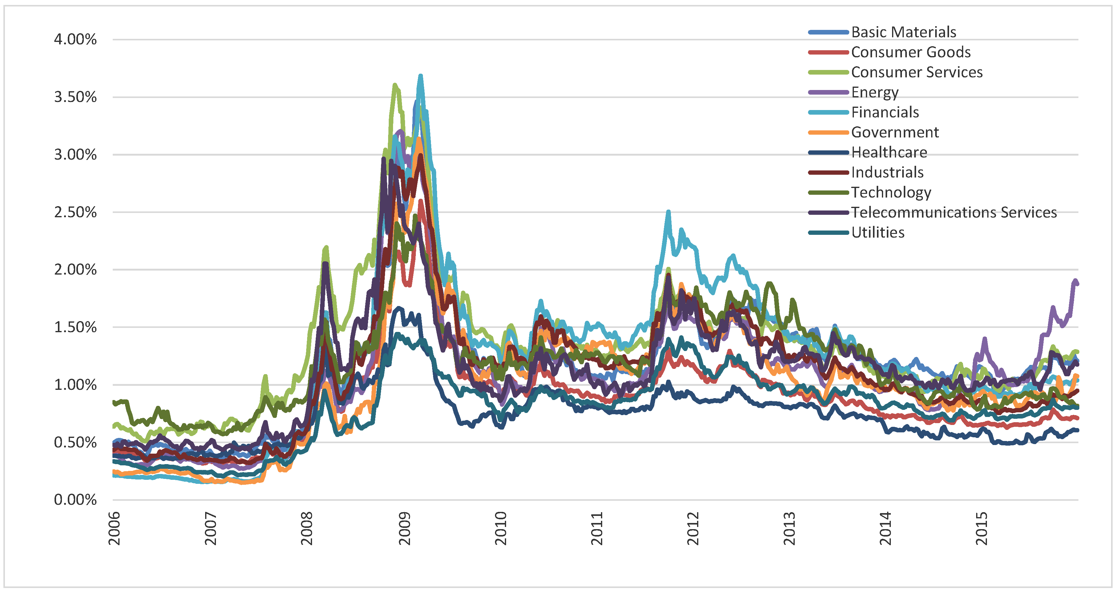
3.2.2. Time Evolution
3.2.3. The Relationship of Sectorial CDS Indices with Credit and Equity Market Indices
4. Estimating a Global Risk Factor
4.1. Estimation Methodology
4.2. The Information Content of the Global Risk Factor
5. Systemic, Sectorial and Idiosyncratic Components of Credit Risk
5.1. Sectorial Portfolios
5.2. Decomposition of Risk at the Level of the Firm
5.2.1. European Financial and Industrial Sectors
5.2.2. North American Financial and Industrial Sectors
6. An Evaluation of the Proposed Methodology for Risk Decomposition
6.1. Two Validation Tests
6.2. Diversification Strategies Based on Estimated Idiosyncratic Components
6.3. Idiosyncratic Risk and Lack of Liquidity
7. Robustness Tests
8. Synthetic Factor Regressions
9. Conclusions
Author Contributions
Funding
Acknowledgments
Conflicts of Interest
References
- Acharya, Viral, Itamar Drechsler, and Philipp Schnabl. 2014. A pyrrhic victory? Bank bailouts and sovereign credit risk. The Journal of Finance 69: 2689–739. [Google Scholar] [CrossRef]
- Badaoui, Saad, Lara Cathcart, and Lina El-Jahel. 2013. Do sovereign credit default swaps represent a clean measure of sovereign default risk? A factor model approach. Journal of Banking & Finance 37: 2392–407. [Google Scholar]
- Ballester, Laura, Barbara Casu, and Ana González-Urteaga. 2016. Bank fragility and contagion: Evidence from the bank CDS market. Journal of Empirical Finance 38: 394–416. [Google Scholar] [CrossRef]
- BCBS. 2000. Principles for the Management of Credit Risk. Basel: Basel Committee on Banking Supervision. [Google Scholar]
- BCBS. 2011. Basel III: A Global Regulatory Framework for More Resilient Banks and Banking Systems. Basel: Basel Committee on Banking Supervision. [Google Scholar]
- BCBS. 2012. A Framework for Dealing with Domestic Systemically Important Banks. Basel: Basel Committee on Banking Supervisions. [Google Scholar]
- Beirne, John. 2012. The EONIA spread before and during the crisis of 2007–2009: The role of liquidity and credit risk. Journal of International Money and Finance 31: 534–51. [Google Scholar] [CrossRef]
- Berndt, Antje, and Iulian Obreja. 2010. Decomposing European CDS returns. Review of Finance 14: 189–233. [Google Scholar] [CrossRef]
- Bhansali, Vineer, Robert Gingrich, and Francis A. Longstaff. 2008. Systemic credit risk: What is the market telling us? Financial Analysts Journal 64: 16–24. [Google Scholar] [CrossRef]
- Blix Grimaldi, Marianna. 2010. Detecting and Interpreting Financial Stress in the Euro Area. Technical Report, ECB Working Paper. Frankfurt: ECB. [Google Scholar]
- Campa, Jose Manuel, and PH Kevin Chang. 1998. The forecasting ability of correlations implied in foreign exchange options. Journal of International Money and Finance 17: 855–80. [Google Scholar] [CrossRef]
- Chen, Cathy Yi-Hsuan, and Wolfgang Karl Härdle. 2015. Common factors in credit defaults swap markets. Computational Statistics 30: 845–63. [Google Scholar] [CrossRef]
- Driessen, Joost, Pascal J. Maenhout, and Grigory Vilkov. 2009. The price of correlation risk: Evidence from equity options. The Journal of Finance 64: 1377–406. [Google Scholar] [CrossRef]
- Duellmann, Klaus, and Nancy Masschelein. 2007. A tractable model to measure sector concentration risk in credit portfolios. Journal of Financial Services Research 32: 55–79. [Google Scholar] [CrossRef]
- EBA. 2014. On the Minimum List of Qualitative and Quantitative Recovery Plan Indicators. Paris: European Banking Authority. [Google Scholar]
- Eder, Armin, and Sebastian Keiler. 2015. CDS spreads and contagion amongst systemically important financial institutions—A spatial econometric approach. International Journal of Finance & Economics 20: 291–309. [Google Scholar]
- Eichengreen, Barry, Ashoka Mody, Milan Nedeljkovic, and Lucio Sarno. 2012. How the subprime crisis went global: Evidence from bank credit default swap spreads. Journal of International Money and Finance 31: 1299–318. [Google Scholar] [CrossRef]
- FSB. 2013. Principles for an Effective Risk Appetite Framework. Basel: Financial Stability Board. [Google Scholar]
- Giglio, Stefano. 2010. CDS Spreads and Systemic Financial Risk. Ph.D. thesis, Harvard University, Cambridge, CA, USA. [Google Scholar]
- Gropp, Reint, Jukka Vesala, and Giuseppe Vulpes. 2006. Equity and bond market signals as leading indicators of bank fragility. Journal of Money, Credit and Banking 38: 399–428. [Google Scholar] [CrossRef]
- Hammoudeh, Shawkat, Mohan Nandha, and Yuan Yuan. 2013. Dynamics of CDS spread indexes of US financial sectors. Applied Economics 45: 213–23. [Google Scholar] [CrossRef]
- Heinz, Frigyes F., and Yan Sun. 2014. Sovereign CDS Spreads in Europe: The Role of Global Risk Aversion, Economic Fundamentals, Liquidity, and Spillovers. Number 14–17. Washington, DC: International Monetary Fund. [Google Scholar]
- Heitfield, Eric, Steve Burton, and Souphala Chomsisengphet. 2006. Systematic and idiosyncratic risk in syndicated loan portfolios. Journal of Credit Risk 2: 3–31. [Google Scholar] [CrossRef]
- Hilscher, Jens, and Yves Nosbusch. 2010. Determinants of sovereign risk: Macroeconomic fundamentals and the pricing of sovereign debt. Review of Finance 14: 235–62. [Google Scholar] [CrossRef]
- Hui, Cho-Hoi, Chi-Fai Lo, and Chun-Sing Lau. 2013. Option-implied correlation between iTraxx europe financials and non-financials indexes: A measure of spillover effect in european debt crisis. Journal of Banking & Finance 37: 3694–703. [Google Scholar]
- Hull, John, Mirela Predescu, and Alan White. 2004. The relationship between credit default swap spreads, bond yields, and credit rating announcements. Journal of Banking & Finance 28: 2789–811. [Google Scholar]
- Illing, Mark, and Meyer Aaron. 2005. A brief survey of risk-appetite indexes. In Bank of Canada Financial Stability Review. Ottawa: Bank of Canada. [Google Scholar]
- Longstaff, Francis A., Jun Pan, Lasse H. Pedersen, and Kenneth J. Singleton. 2011. How sovereign is sovereign credit risk? American Economic Journal: Macroeconomics 3: 75–103. [Google Scholar] [CrossRef]
- Lopez, Jose, and Christian Walter. 2000. Is implied correlation worth calculating? evidence from foreign exchange options and historical data. Journal of Derivatives 7: 65–81. [Google Scholar]
- Markit. 2008. Markit.com User Guide. Version 14.3. London: IHS Markit. [Google Scholar]
- Markit. 2012. Markit.com User Guide CDS & Bonds. Version 16. London: IHS Markit. [Google Scholar]
- Munves, David W. 2008. Financial Sector Risk Dominates the Credit Default Swap Market. Viewpoint: Moody’s Capital Markets Research Group. [Google Scholar]
- Ornelas, José Renato Haas. 2019. Expected currency returns and volatility risk premia. The North American Journal of Economics and Finance 49: 206–34. [Google Scholar] [CrossRef]
- Puzanova, Natalia, and Klaus Düllmann. 2013. Systemic risk contributions: A credit portfolio approach. Journal of Banking & Finance 37: 1243–57. [Google Scholar]
- Pykhtin, Michael. 2004. Portfolio credit risk multi-factor adjustment. Risk 17: 85–90. [Google Scholar]
- Rodríguez-Moreno, María, and Juan Ignacio Peña. 2013. Systemic risk measures: The simpler the better? Journal of Banking & Finance 37: 1817–31. [Google Scholar]
- Schwaab, Bernd, Siem Jan Koopman, and André Lucas. 2017. Global credit risk: World, country and industry factors. Journal of Applied Econometrics 32: 296–317. [Google Scholar] [CrossRef]
- Siegel, Andrew F. 1997. International currency relationship information revealed by cross-option prices. The Journal of Futures Markets (1986–1998) 17: 369. [Google Scholar] [CrossRef]
- Skintzi, Vasiliki D., and Apostolos-Paul N. Refenes. 2005. Implied correlation index: A new measure of diversification. Journal of Futures Markets: Futures, Options, and Other Derivative Products 25: 171–97. [Google Scholar] [CrossRef]
- Thornton, Daniel L. 2009. What the Libor-OIS Spread Says. Economic Synopses, 24. St. Louis: Federal Reserve Bank of Saint Louis. [Google Scholar]
| 1 | Government is a category considered by Markit but not included in the Industry Classification Benchmark. |
| 2 | The implicit volatilities from 3-month ATM iTraxx Europe Index Option and the 3-month ATM CDX North American Investment Grade Index Option were provided by JP Morgan. |
| 3 | It is interesting to note that the government sector seems to have a strong specific behavior that explains its association with the second principal component in spite of having a loading in the first component in line with that of the other sectors. |
| 4 | A decision in line with other authors, like Rodríguez-Moreno and Peña (2013). |
| 5 | |
| 6 | That correlation was set at 30%, up from the previous value of 24%, while the 24% correlation was kept for the rest of corporate sectors. |
| 7 | Incidentally, remember that the financial sector credit index is the same for European and North American firms. |
| 8 | These are again least-squares, single equation estimates. |
| 9 | With a number of firms between 26 and 52 in each sector, statistical significance would require correlation coefficients above 0.30 in absolute value. |
| 10 | Had we used firm-specific indicators, like the price of the firm’s stock, or some indicator of the accounting results of the firm, we would expect to have the more idiosyncratic firms to be very responsive to such indicators. |


| Variable | Mean | Median | St. Dev. | Minimum | Maximum | DFA(1) |
|---|---|---|---|---|---|---|
| Euribor 3m | 1.64 | 0.91 | 1.67 | −0.19 | 5.38 | −0.70 |
| Eonia 3m | 1.31 | 0.47 | 1.57 | −0.31 | 4.34 | −0.54 |
| USD Libor 3m | 1.60 | 0.38 | 1.99 | 0.22 | 5.71 | −1.57 |
| USD OIS 3m | 1.29 | 0.17 | 1.97 | 0.07 | 5.41 | −1.74 |
| Euro swap 1y | 1.84 | 1.26 | 1.65 | −0.13 | 5.42 | −0.21 |
| Euro swap 5y | 2.35 | 2.35 | 1.45 | 0.11 | 5.15 | 0.02 |
| Euro swap 10y | 2.89 | 3.16 | 1.26 | 0.46 | 5.07 | 0.15 |
| USD swap 1y | 1.67 | 0.54 | 1.91 | 0.26 | 5.72 | −1.63 |
| USD swap 5y | 2.62 | 1.98 | 1.48 | 0.75 | 5.72 | −1.28 |
| USD swap 10y | 3.36 | 3.04 | 1.21 | 1.57 | 5.82 | −1.13 |
| Japan swap 1y | 0.47 | 0.36 | 0.29 | 0.00 | 1.14 | −0.49 |
| Japan swap 5y | 0.74 | 0.58 | 0.45 | 0.00 | 1.70 | −0.53 |
| Japan swap 10y | 1.21 | 1.18 | 0.48 | 0.24 | 2.23 | −0.48 |
| MSCI World/Basic materials | 229.65 | 228.91 | 38.35 | 119.01 | 334.81 | −2.34 |
| MSCI World/Consumer goods | 146.98 | 136.43 | 34.13 | 85.78 | 211.15 | −0.44 |
| MSCI World/Consumer services | 128.28 | 119.94 | 36.86 | 55.59 | 202.76 | −0.48 |
| MSCI World/Energy | 239.56 | 238.48 | 34.32 | 148.49 | 335.24 | −2.34 |
| MSCI World/Financial | 99.80 | 95.06 | 30.03 | 38.44 | 166.56 | −1.33 |
| MSCI World/Healthcare | 129.83 | 113.95 | 39.74 | 72.08 | 227.38 | −0.00 |
| MSCI World/Industrials, | 158.21 | 157.77 | 31.09 | 72.59 | 208.88 | −1.41 |
| MSCI World/Technology | 96.46 | 90.90 | 24.33 | 47.40 | 150.62 | −0.50 |
| MSCI World/Telecommunication services | 61.50 | 60.50 | 8.68 | 41.26 | 81.52 | −1.73 |
| MSCI World/Utility | 117.50 | 111.91 | 17.50 | 85.65 | 168.79 | −1.70 |
| Liquidity USD Premium (USD Libor 3m-USD OIS 3m) | 0.31 | 0.15 | 0.40 | 0.05 | 3.43 | −4.28 |
| Liquidity Euro premium (Euribor 3m-Eonia 3m) | 0.33 | 0.20 | 0.33 | 0.05 | 1.85 | −2.81 |
| USD Swaption 3m5y | 94.16 | 81.81 | 35.97 | 41.64 | 208.15 | −2.34 |
| Euro Swaption 3m5y | 69.93 | 66.36 | 25.35 | 26.92 | 166.75 | −2.41 |
| VIX Index | 20.39 | 17.38 | 9.69 | 10.18 | 72.92 | −3.14 |
| VSTOXX | 24.53 | 22.45 | 9.16 | 13.22 | 71.49 | −3.69 |
| Imp Vol 3m EURUSD fx | 10.30 | 10.08 | 3.43 | 4.90 | 23.56 | −2.05 |
| Imp Vol 3m Itraxx IG | 0.64 | 0.60 | 0.24 | 0.00 | 1.44 | −3.60 |
| Imp Vol 3m CDX IG | 0.58 | 0.53 | 0.21 | 0.00 | 1.15 | −3.42 |
| EURUSD fx | 1.33 | 1.33 | 0.11 | 1.06 | 1.59 | −1.81 |
| JPYUSD Fx | 0.01 | 0.01 | 0.00 | 0.01 | 0.01 | −1.12 |
| German Government Bond 5y | 1.90 | 1.78 | 1.48 | −0.25 | 4.70 | −0.33 |
| German Government Bond 10Y | 2.57 | 2.76 | 1.25 | 0.09 | 4.64 | −0.33 |
| US Treasury bond 5y | 2.26 | 1.73 | 1.32 | 0.58 | 5.18 | −1.49 |
| US Treasury bond 10y | 3.10 | 2.90 | 1.03 | 1.44 | 5.21 | −1.49 |
| Japan Government Bond 10y | 1.10 | 1.15 | 0.47 | 0.07 | 1.98 | −0.30 |
| US slope | 1.69 | 1.71 | 0.99 | −0.25 | 3.34 | −1.82 |
| EUR slope | 1.05 | 1.11 | 0.72 | −0.48 | 2.39 | −1.42 |
| Yen slope | 0.75 | 0.69 | 0.30 | 0.23 | 1.77 | −2.19 |
| US curvature | −0.21 | −0.18 | 0.51 | −1.50 | 0.56 | −2.11 |
| EUR curvature | 0.04 | 0.14 | 0.35 | −0.91 | 0.73 | −1.96 |
| Yen curvature | 0.21 | 0.27 | 0.24 | −0.64 | 0.49 | −1.94 |
| Itraxx IG | 90.96 | 89.07 | 44.19 | 20.56 | 204.24 | −2.11 |
| CDX IG | 90.96 | 85.41 | 42.17 | 29.96 | 264.60 | −2.33 |
| Itraxx Japan IG | 111.37 | 96.92 | 81.73 | 14.75 | 542.98 | −2.61 |
| HiVol Itraxx | 143.62 | 136.76 | 87.63 | 39.69 | 500.58 | −2.00 |
| CDX HY | 522.60 | 447.84 | 264.75 | 188.54 | 1775.51 | −2.13 |
| Variable | Mean | Median | St. Dev. | Minimum | Maximum | DFA(1) |
|---|---|---|---|---|---|---|
| Euribor 3m | −0.005 | −0.001 | 0.05 | −0.33 | 0.21 | −7.94 |
| Eonia 3m | −0.005 | 0.000 | 0.05 | −0.40 | 0.09 | −7.90 |
| USD Libor 3m | −0.008 | 0.000 | 0.09 | −0.87 | 0.64 | −11.23 |
| USD OIS 3m | −0.008 | 0.000 | 0.05 | −0.55 | 0.09 | −7.85 |
| USD swap 1y | −0.008 | −0.002 | 0.07 | −0.39 | 0.42 | −12.22 |
| USD swap 5y | −0.007 | −0.012 | 0.10 | −0.40 | 0.48 | −13.29 |
| USD swap 10y | −0.006 | −0.008 | 0.11 | −0.53 | 0.38 | −13.39 |
| Euro swap 1y | −0.006 | −0.002 | 0.06 | −0.27 | 0.21 | −9.78 |
| Euro swap 5y | −0.006 | −0.007 | 0.07 | −0.29 | 0.30 | −14.00 |
| Euro swap 10y | −0.005 | −0.009 | 0.08 | −0.39 | 0.28 | −14.95 |
| Japan swap 1y | 0.000 | 0.000 | 0.02 | −0.11 | 0.10 | −13.16 |
| Japan swap 5y | −0.002 | −0.003 | 0.04 | −0.18 | 0.15 | −14.05 |
| Japan swap 10y | −0.003 | −0.005 | 0.04 | −0.20 | 0.15 | −14.77 |
| MSCI World/Basic materials | −0.016 | 0.442 | 6.68 | −36.80 | 18.56 | −15.36 |
| MSCI World/Consumer goods | 0.200 | 0.403 | 2.02 | −12.82 | 5.73 | −15.07 |
| MSCI World/Consumer services | 0.144 | 0.534 | 2.49 | −12.81 | 7.28 | −14.66 |
| MSCI World/Energy | −0.072 | 0.580 | 6.62 | −37.95 | 17.50 | −15.77 |
| MSCI World/Financial | −0.088 | 0.272 | 2.56 | −15.47 | 8.40 | −15.20 |
| MSCI World/Healthcare | 0.171 | 0.306 | 2.22 | −16.14 | 8.83 | −15.82 |
| MSCI World/Industrials, | 0.087 | 0.520 | 3.32 | −17.96 | 9.15 | −14.93 |
| MSCI World/Technology | 0.110 | 0.354 | 1.97 | −9.38 | 5.74 | −14.35 |
| MSCI World/Telecommunication services | 0.028 | 0.140 | 1.06 | −5.93 | 3.31 | −15.01 |
| MSCI World/Utility | 0.010 | 0.272 | 2.15 | −17.15 | 6.10 | −16.19 |
| Liquidity USD Premium (USD Libor 3m-USD OIS 3m) | 0.000 | 0.000 | 0.08 | −0.75 | 0.88 | −11.59 |
| Liquidity Euro premium (Euribor 3m-Eonia 3m) | 0.000 | −0.001 | 0.05 | −0.26 | 0.49 | −12.21 |
| USD Swaption 3m5y | −0.009 | −0.288 | 6.07 | −24.49 | 34.00 | −14.54 |
| Euro Swaption 3m5y | −0.044 | −0.140 | 4.22 | −24.19 | 24.90 | −16.80 |
| VIX Index | 0.017 | −0.122 | 2.65 | −14.77 | 16.16 | −15.98 |
| VSTOXX | 0.027 | −0.117 | 2.93 | −16.02 | 19.20 | −16.45 |
| Vol Imp 3m EURUSD fx | 0.002 | −0.021 | 0.63 | −2.52 | 4.98 | −16.47 |
| Vol Imp 3m Itraxx IG | 0.001 | −0.002 | 0.05 | −0.23 | 0.38 | −15.10 |
| Vol Imp 3m CDX IG | 0.001 | −0.001 | 0.04 | −0.15 | 0.43 | −14.32 |
| EURUSD fx | 0.000 | 0.000 | 0.02 | −0.06 | 0.09 | −14.17 |
| JPYUSD Fx | 0.000 | 0.000 | 0.00 | 0.00 | 0.00 | −13.63 |
| German Government Bond 5y | −0.006 | −0.005 | 0.09 | −0.34 | 0.25 | −14.51 |
| German Government Bond 10Y | −0.005 | −0.009 | 0.08 | −0.30 | 0.31 | −15.27 |
| US Treasury bond 5y | −0.006 | −0.008 | 0.10 | −0.40 | 0.35 | −13.19 |
| US Treasury bond 10y | −0.004 | −0.009 | 0.10 | −0.41 | 0.33 | −13.38 |
| Japan Government Bond 10y | −0.003 | −0.004 | 0.04 | −0.21 | 0.14 | −15.04 |
| US slope | 0.002 | −0.005 | 0.10 | −0.48 | 0.34 | −13.61 |
| EUR slope | 0.000 | −0.005 | 0.07 | −0.22 | 0.36 | −14.34 |
| Yen slope | −0.002 | −0.004 | 0.04 | −0.18 | 0.14 | −15.05 |
| US curvature | 0.000 | 0.005 | 0.08 | −0.28 | 0.28 | −13.71 |
| EUR curvature | 0.001 | 0.002 | 0.05 | −0.24 | 0.18 | −15.07 |
| Yen curvature | 0.001 | 0.000 | 0.03 | −0.15 | 0.12 | −14.00 |
| Itraxx IG | 0.106 | −0.128 | 6.88 | −22.91 | 30.27 | −15.15 |
| CDX IG | 0.104 | −0.215 | 6.83 | −41.11 | 41.66 | −15.78 |
| Itraxx Japan IG | 0.122 | −0.195 | 13.50 | −93.52 | 66.92 | −14.76 |
| HiVol Itraxx | 0.076 | −0.331 | 12.31 | −61.54 | 87.86 | −14.72 |
| CDX HY | 0.003 | −0.016 | 0.37 | −2.14 | 2.48 | −14.35 |
| Statistic | BM | CG | CS | EN | FIN | GOV | HC | IND | TEC | TEL | UTI |
|---|---|---|---|---|---|---|---|---|---|---|---|
| Mean*100 | 0.171 | 0.106 | 0.135 | 0.303 | 0.304 | 0.282 | 0.087 | 0.150 | −0.008 | 0.174 | 0.168 |
| Standard deviation*100 | 4.15 | 3.82 | 3.92 | 4.29 | 4.57 | 5.42 | 3.96 | 4.02 | 4.09 | 5.13 | 3.46 |
| Volatility | 29.9% | 27.5% | 28.3% | 30.9% | 32.9% | 39.1% | 28.6% | 29.0% | 29.5% | 37.0% | 24.9% |
| Skewness | 0.69 | 0.71 | 0.38 | 0.85 | 1.65 | 1.18 | 0.64 | 0.78 | 0.29 | 0.67 | 1.29 |
| Kurtosis | 5.43 | 6.88 | 4.96 | 6.73 | 11.84 | 9.28 | 9.52 | 6.36 | 3.86 | 5.31 | 8.91 |
| Maximum | 0.20 | 0.19 | 0.18 | 0.24 | 0.30 | 0.34 | 0.23 | 0.19 | 0.16 | 0.20 | 0.19 |
| minimum | −0.14 | −0.16 | −0.15 | −0.18 | −0.16 | −0.22 | −0.21 | −0.15 | −0.11 | −0.19 | −0.11 |
| Range | 0.34 | 0.35 | 0.33 | 0.42 | 0.46 | 0.56 | 0.43 | 0.34 | 0.28 | 0.39 | 0.31 |
| Jarque–Bera | 168.7 | 369.8 | 96.0 | 363.9 | 1933.4 | 978.0 | 958.2 | 297.0 | 23.5 | 154.0 | 902.7 |
| Unit Root Tests | |||||||||||
| Index levels | |||||||||||
| adf1 | −2.09 | −1.97 | −1.90 | −1.91 | −1.92 | −2.06 | −2.18 | −1.83 | −1.83 | −2.38 | −1.76 |
| adf4 | −2.28 | −2.25 | −2.20 | −2.11 | −2.16 | −2.18 | −2.37 | −2.05 | −1.87 | −2.34 | −2.09 |
| adf8 | −2.38 | −2.08 | −2.29 | −2.69 | −2.23 | −2.54 | −2.42 | −2.40 | −1.92 | −2.82 | −2.01 |
| Weekly changes | |||||||||||
| adf1 | −12.18 | −13.57 | −13.85 | −12.35 | −11.32 | −13.86 | −15.45 | −12.88 | −14.80 | −14.50 | −12.15 |
| adf4 | −8.65 | −8.66 | −8.88 | −7.46 | −8.74 | −8.71 | −8.23 | −8.23 | −9.18 | −10.12 | −8.36 |
| adf8 | −6.98 | −6.98 | −6.84 | −5.76 | −7.06 | −6.52 | −6.80 | −6.45 | −7.58 | −6.95 | −7.10 |
| Sector | BM | CG | CS | EN | FIN | GOV | HC | IND | TEC | TEL | UTI |
|---|---|---|---|---|---|---|---|---|---|---|---|
| BM | 100% | 73% | 67% | 67% | 68% | 61% | 47% | 76% | 54% | 62% | 64% |
| CG | 73% | 100% | 71% | 69% | 77% | 65% | 49% | 80% | 56% | 67% | 73% |
| CS | 67% | 71% | 100% | 65% | 66% | 57% | 44% | 71% | 47% | 66% | 64% |
| EN | 67% | 69% | 65% | 100% | 73% | 62% | 46% | 70% | 51% | 64% | 71% |
| FIN | 68% | 77% | 66% | 73% | 100% | 72% | 49% | 77% | 53% | 67% | 76% |
| GOV | 61% | 65% | 57% | 62% | 72% | 100% | 35% | 67% | 47% | 56% | 65% |
| HC | 47% | 49% | 44% | 46% | 49% | 35% | 100% | 52% | 35% | 42% | 48% |
| IND | 76% | 80% | 71% | 70% | 77% | 67% | 52% | 100% | 55% | 67% | 72% |
| TEC | 54% | 56% | 47% | 51% | 53% | 47% | 35% | 55% | 100% | 50% | 51% |
| TEL | 62% | 67% | 66% | 64% | 67% | 56% | 42% | 67% | 50% | 100% | 66% |
| UTI | 64% | 73% | 64% | 71% | 76% | 65% | 48% | 72% | 51% | 66% | 100% |
| Median | 67% | 71% | 66% | 67% | 72% | 62% | 47% | 71% | 51% | 66% | 66% |
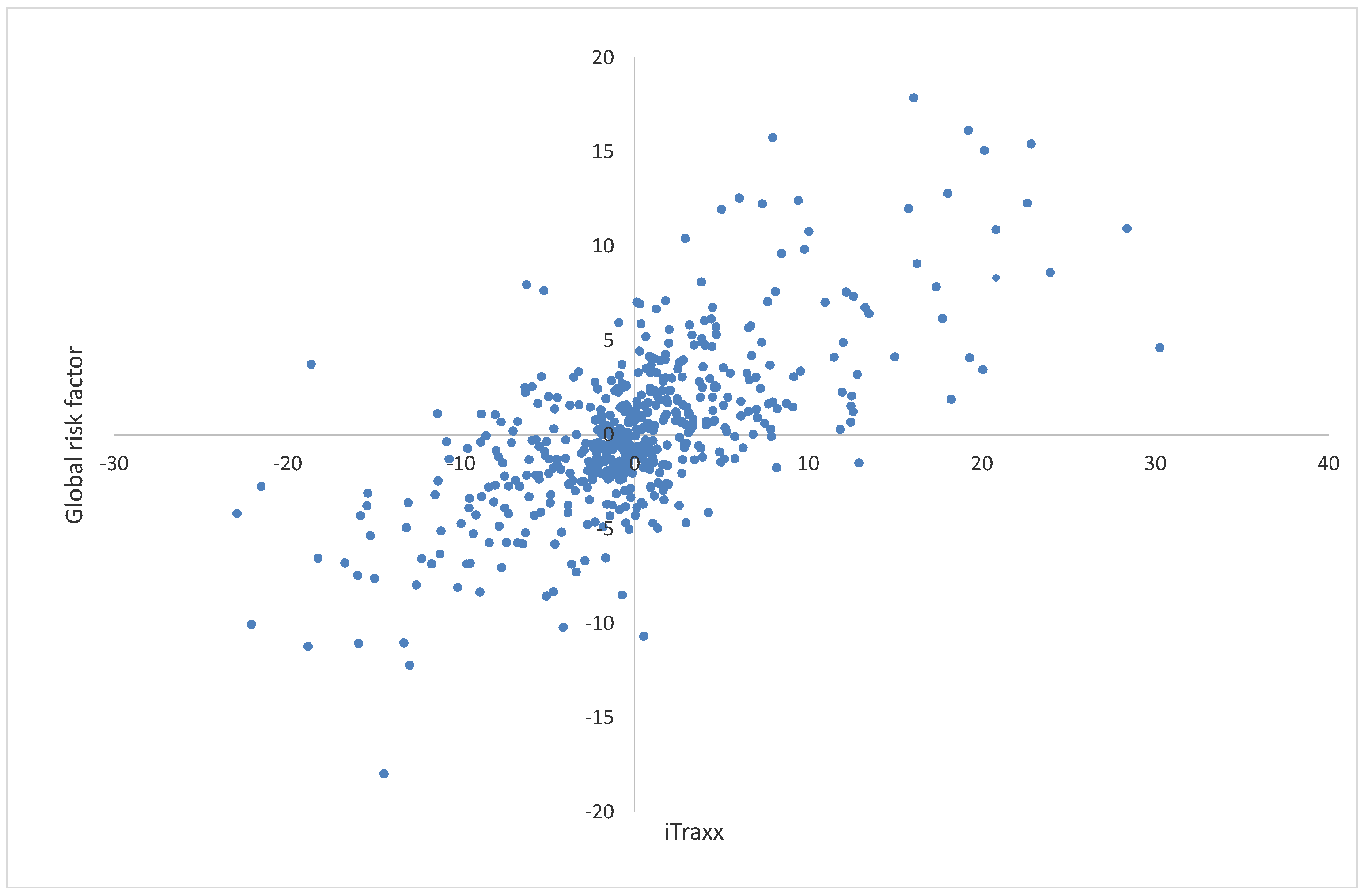
| Factor: iTraxx | Beta | adj R2 | *100 | Jarque–Bera | LBQ(1) | LBQ(4) | LBQ(12) | Arch Test | ADF(1) |
|---|---|---|---|---|---|---|---|---|---|
| BM | 0.35 | 0.34 | 3.37 | 228.5 | 9.9 | 20.5 | 28.2 | 8.6 | −13.8 |
| CG | 0.38 | 0.47 | 2.78 | 207.1 | 25.8 | 27.9 | 45.0 | 43.6 | −15.2 |
| CS | 0.35 | 0.39 | 3.07 | 92.7 | 6.3 | 7.0 | 16.0 | 2.6 | −15.7 |
| EN | 0.38 | 0.37 | 3.41 | 264.7 | 59.2 | 79.6 | 98.4 | 90.4 | −13.0 |
| FIN | 0.48 | 0.53 | 3.13 | 2394.8 | 85.9 | 138.5 | 142.4 | 165.6 | −11.3 |
| GOV | 0.44 | 0.32 | 4.49 | 1089.4 | 12.7 | 15.3 | 22.1 | 19.4 | −14.9 |
| HC | 0.27 | 0.22 | 3.51 | 369.3 | 2.2 | 6.2 | 18.0 | 0.9 | −16.9 |
| IND | 0.39 | 0.44 | 3.01 | 276.8 | 17.7 | 20.7 | 45.3 | 24.3 | −13.9 |
| TEC | 0.29 | 0.24 | 3.56 | 38.5 | 0.1 | 3.4 | 10.6 | 28.2 | −16.3 |
| TEL | 0.51 | 0.47 | 3.75 | 34.7 | 6.8 | 13.9 | 22.2 | 14.9 | −16.0 |
| UTI | 0.33 | 0.44 | 2.58 | 340.2 | 25.9 | 46.4 | 57.8 | 18.4 | −14.0 |
| Sector | MSCI | MSCI + iTraxx | MSCI + GRF | All Indicators |
|---|---|---|---|---|
| BM | 0.30 | 0.38 | 0.70 | 0.52 |
| CG | 0.36 | 0.50 | 0.77 | 0.65 |
| CS | 0.34 | 0.43 | 0.65 | 0.53 |
| EN | 0.37 | 0.43 | 0.70 | 0.53 |
| FIN | 0.43 | 0.57 | 0.79 | 0.72 |
| GOV | 0.28 | 0.35 | 0.65 | 0.43 |
| HC | 0.17 | 0.24 | 0.36 | 0.28 |
| IND | 0.36 | 0.48 | 0.79 | 0.59 |
| TEC | 0.19 | 0.25 | 0.43 | 0.31 |
| TEL | 0.39 | 0.51 | 0.67 | 0.56 |
| UTI | 0.31 | 0.46 | 0.70 | 0.55 |
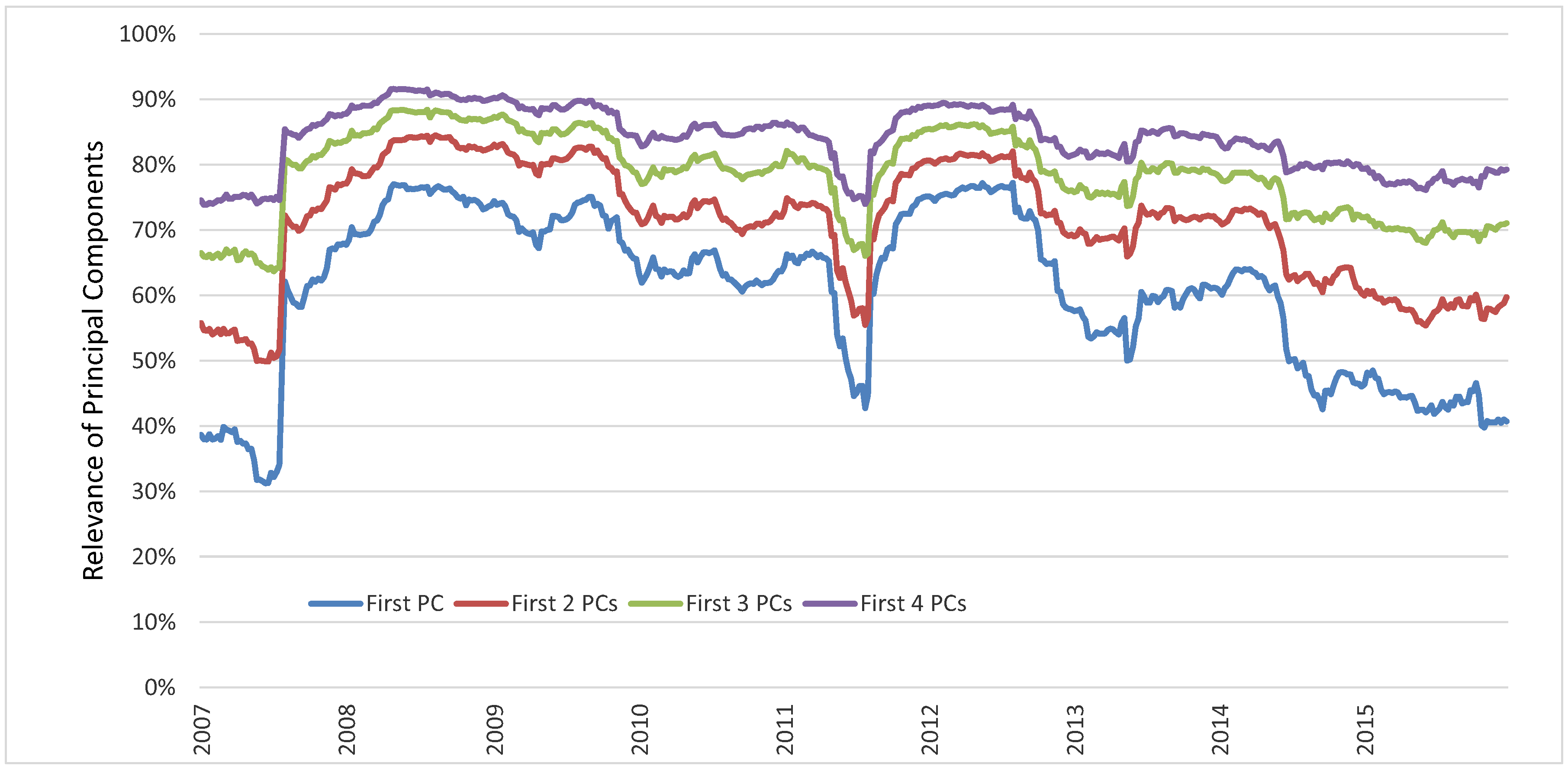
| Eigenvalue Order | Eigenvalue | Cumulative Variance | Sector | First Eigenv. | Second Eigenv. | Third Eigenv. | Fourth Eigenv. |
|---|---|---|---|---|---|---|---|
| 1 | 0.0133 | 0.654 | BM | 0.299 | −0.079 | 0.086 | 0.121 |
| 2 | 0.0014 | 0.722 | CG | 0.291 | −0.055 | 0.023 | 0.033 |
| 3 | 0.0011 | 0.776 | CS | 0.274 | −0.148 | −0.107 | −0.113 |
| 4 | 0.0010 | 0.827 | EN | 0.311 | −0.032 | 0.004 | −0.059 |
| 5 | 0.0008 | 0.866 | FIN | 0.352 | 0.123 | 0.097 | −0.086 |
| 6 | 0.0007 | 0.899 | GOV | 0.380 | 0.791 | 0.102 | −0.077 |
| 7 | 0.0005 | 0.926 | HC | 0.200 | −0.448 | 0.716 | −0.193 |
| 8 | 0.0005 | 0.951 | IND | 0.309 | −0.051 | 0.084 | 0.012 |
| 9 | 0.0004 | 0.968 | TEC | 0.234 | −0.123 | −0.055 | 0.915 |
| 10 | 0.0003 | 0.985 | TEL | 0.363 | −0.330 | −0.661 | −0.275 |
| 11 | 0.0003 | 1 | UTI | 0.251 | −0.001 | 0.023 | −0.068 |
| Factor: GRF | Beta | adj R2 | *100 | Jarque–Bera | LBQ(1) | LBQ(4) | LBQ(12) | Arch Test | ADF(1) |
|---|---|---|---|---|---|---|---|---|---|
| BM | 0.30 | 0.70 | 2.28 | 30.1 | 0.0 | 3.2 | 19.9 | 9.4 | −16.6 |
| CG | 0.30 | 0.78 | 1.80 | 51.7 | 9.2 | 19.2 | 31.4 | 6.6 | −17.0 |
| CS | 0.28 | 0.66 | 2.29 | 132.7 | 0.8 | 5.0 | 32.6 | 26.4 | −16.0 |
| EN | 0.31 | 0.70 | 2.36 | 219.5 | 40.4 | 42.7 | 47.0 | 60.7 | −14.3 |
| FIN | 0.36 | 0.79 | 2.11 | 1682.1 | 72.0 | 81.6 | 95.0 | 182.1 | −12.9 |
| GOV | 0.38 | 0.62 | 3.32 | 991.4 | 7.9 | 10.5 | 19.7 | 2.8 | −15.8 |
| HC | 0.21 | 0.35 | 3.19 | 313.7 | 0.5 | 11.4 | 17.2 | 0.2 | −18.0 |
| IND | 0.31 | 0.79 | 1.84 | 52.6 | 0.4 | 12.6 | 23.3 | 3.5 | −17.8 |
| TEC | 0.24 | 0.44 | 3.06 | 42.7 | 0.7 | 6.3 | 22.2 | 40.4 | −16.9 |
| TEL | 0.36 | 0.65 | 3.04 | 136.4 | 1.2 | 6.7 | 26.2 | 16.1 | −16.7 |
| UTI | 0.26 | 0.71 | 1.86 | 115.5 | 9.5 | 12.4 | 38.1 | 25.6 | −15.6 |
| Variable | Correlation | Variable | Correlation | Variable | Correlation |
|---|---|---|---|---|---|
| Libor–OIS spread | −0.327 | iTraxx Japan | −0.212 | MSCI financials | −0.232 |
| Euro swap 1y | −0.204 | high yield CDX | 0.225 | MSCI Industrials | −0.208 |
| US swap 1y | −0.255 | MSCI basic materials | −0.209 | MSCI telecomm. services | −0.204 |
| Firm (1) | Systemic Risk (2) | Sectorial PC (3) | Both (4) | Sectorial Risk (5) | Idiosyncratic Risk (6) |
|---|---|---|---|---|---|
| AXA | 58% | 75% | 76% | 19% | 24% |
| Legal & Gen Gp PLC | 57% | 69% | 71% | 15% | 29% |
| Mediobanca SpA | 56% | 80% | 80% | 25% | 20% |
| Prudential PLC | 55% | 66% | 69% | 14% | 31% |
| Assicurazioni Generali S p A | 52% | 81% | 81% | 29% | 19% |
| Aviva plc | 52% | 75% | 75% | 23% | 25% |
| Rabobank Nederland | 50% | 80% | 80% | 30% | 20% |
| ING Bk N V | 50% | 86% | 86% | 36% | 14% |
| Old Mut plc | 50% | 45% | 54% | 3% | 47% |
| HSBC Bk plc | 50% | 81% | 81% | 31% | 19% |
| Royal & Sun Alliance Ins PLC | 49% | 70% | 70% | 21% | 30% |
| Bca Pop di Milano Soc Coop a r l | 49% | 76% | 76% | 27% | 24% |
| Munich Re | 49% | 78% | 78% | 29% | 22% |
| Bca Monte dei Paschi di Siena S p A | 48% | 76% | 76% | 29% | 24% |
| Bca Naz del Lavoro S p A | 47% | 80% | 80% | 33% | 20% |
| Std Chartered Bk | 46% | 73% | 73% | 27% | 27% |
| Societe Generale | 45% | 83% | 84% | 39% | 16% |
| STANDARD CHARTERED PLC | 45% | 71% | 71% | 26% | 29% |
| BNP Paribas | 45% | 86% | 87% | 41% | 13% |
| ACE Ltd | 44% | 35% | 45% | 1% | 55% |
| Aegon N.V. | 44% | 60% | 60% | 17% | 40% |
| Skandinaviska Enskilda Banken AB | 43% | 60% | 60% | 17% | 40% |
| UBS AG | 43% | 78% | 78% | 35% | 22% |
| Cr Agricole SA | 43% | 84% | 86% | 43% | 14% |
| Hammerson PLC | 42% | 29% | 42% | 0% | 58% |
| Deutsche Bk AG | 42% | 79% | 80% | 38% | 20% |
| Bco Bilbao Vizcaya Argentaria S A | 42% | 76% | 77% | 35% | 23% |
| Cr LYONNAIS | 42% | 82% | 84% | 42% | 16% |
| Raiffeisen Zentralbank Oesterreich AG | 42% | 46% | 49% | 7% | 51% |
| Inv AB | 41% | 23% | 41% | 0% | 59% |
| Commerzbank AG | 40% | 80% | 81% | 41% | 19% |
| Danske Bk A S | 39% | 59% | 59% | 20% | 41% |
| Nordea Bk AB | 38% | 57% | 57% | 18% | 43% |
| KBC Bk | 38% | 57% | 57% | 19% | 43% |
| Barclays Bk plc | 38% | 80% | 82% | 44% | 18% |
| Bco Comercial Portugues SA | 36% | 69% | 70% | 35% | 30% |
| Royal Bk of Scotland Pub Ltd Co | 36% | 75% | 77% | 41% | 23% |
| Klepierre | 35% | 21% | 35% | 0% | 65% |
| Gecina | 35% | 37% | 40% | 5% | 60% |
| 3i Gp plc | 34% | 21% | 34% | 0% | 66% |
| ISS Glob A S | 32% | 28% | 33% | 1% | 67% |
| Bco de Sabadell S A | 31% | 51% | 51% | 20% | 49% |
| Svenska Handelsbanken AB | 31% | 50% | 50% | 19% | 50% |
| Dexia Cr Loc | 28% | 58% | 60% | 32% | 40% |
| Bay Landbk Giroz | 26% | 50% | 51% | 24% | 50% |
| Landbk Baden Wuertbg | 25% | 39% | 38% | 14% | 62% |
| Nationwide Bldg Soc | 24% | 45% | 45% | 21% | 55% |
| Brit Ld Co plc | 21% | 11% | 21% | 0% | 79% |
| DZ Bk AG | 21% | 23% | 25% | 4% | 75% |
| IKB Deutsche Industriebank AG | 14% | 22% | 22% | 8% | 78% |
| Ld Secs PLC | 12% | 8% | 12% | 0% | 88% |
| Storebrand ASA | 8% | 6% | 8% | 0% | 92% |
| Firm (1) | Systemic Risk (2) | Sectorial Risk (2) | Both (4) | Sectorial Risk (5) | Idiosyncratic Risk (6) |
|---|---|---|---|---|---|
| Cie de St Gobain | 65% | 79% | 79% | 13% | 21% |
| THALES | 62% | 77% | 77% | 15% | 23% |
| Lafarge | 62% | 74% | 74% | 13% | 26% |
| Vinci | 59% | 74% | 74% | 15% | 26% |
| Adecco S A | 59% | 69% | 69% | 10% | 31% |
| AB Volvo | 59% | 74% | 74% | 15% | 26% |
| BAE Sys PLC | 56% | 70% | 70% | 14% | 30% |
| ASSA ABLOY AB | 56% | 59% | 60% | 4% | 40% |
| Atlas Copco AB | 56% | 56% | 59% | 3% | 41% |
| Rexam plc | 55% | 63% | 63% | 8% | 37% |
| Volvo Treas AB | 55% | 66% | 66% | 12% | 34% |
| SCANIA AB | 55% | 63% | 63% | 9% | 37% |
| Metso Corp | 54% | 59% | 60% | 6% | 40% |
| Siemens AG | 53% | 58% | 59% | 6% | 41% |
| Finmeccanica S p A | 52% | 66% | 66% | 14% | 34% |
| ROLLSROYCE PLC | 51% | 68% | 68% | 17% | 32% |
| Deutsche Lufthansa AG | 49% | 63% | 64% | 15% | 36% |
| SOCIETE AIR FRANCE | 49% | 60% | 60% | 12% | 40% |
| HeidelbergCement AG | 48% | 60% | 60% | 12% | 40% |
| Securitas AB | 47% | 56% | 56% | 9% | 44% |
| Deutsche Post AG | 46% | 57% | 57% | 11% | 43% |
| ALSTOM | 44% | 56% | 56% | 12% | 44% |
| Brit Awys plc | 44% | 52% | 52% | 8% | 48% |
| AB SKF | 43% | 43% | 45% | 2% | 55% |
| Smiths Gp Plc | 39% | 48% | 48% | 9% | 52% |
| Rentokil Initial 1927 Plc | 25% | 31% | 31% | 6% | 69% |
| Firm (1) | Systemic Risk (2) | Sectorial PC (3) | Both (4) | Sectorial Risk (5) | Idiosyncratic Risk (6) |
|---|---|---|---|---|---|
| Simon Ppty. Gp. L P | 59% | 64% | 67% | 8% | 33% |
| Simon Ppty. Gp. Inc. | 57% | 60% | 63% | 6% | 37% |
| American Express Co. | 54% | 77% | 77% | 23% | 23% |
| HARTFORD FINL. SERVICES GROUP INC | 54% | 75% | 75% | 22% | 25% |
| Prudential Finl. Inc. | 53% | 74% | 73% | 20% | 27% |
| MetLife Inc. | 53% | 77% | 77% | 24% | 23% |
| Caterpillar Finl. Svcs Corp. | 53% | 53% | 58% | 4% | 42% |
| ERP Oper. Ltd. Pship. | 53% | 58% | 60% | 7% | 40% |
| Avalon Bay Cmntys Inc. | 53% | 54% | 57% | 5% | 43% |
| Berkshire Hathaway Inc. | 52% | 63% | 64% | 12% | 36% |
| General Electric Cap Corp. | 52% | 69% | 69% | 18% | 31% |
| Lincoln Natl. Corp. | 50% | 67% | 67% | 16% | 33% |
| John Deere Cap Corp. | 49% | 51% | 54% | 5% | 46% |
| CNA Finl. Corp. | 48% | 61% | 61% | 13% | 39% |
| Allstate Corp. | 48% | 64% | 64% | 17% | 36% |
| HSBC Fin. Corp. | 47% | 65% | 64% | 17% | 36% |
| INTL. LEASE FIN. CORP. | 45% | 63% | 63% | 18% | 37% |
| DUKE Rlty. Ltd. PARTNERSHIP | 45% | 36% | 45% | 0% | 55% |
| Mack Cali Rlty. LP | 44% | 39% | 45% | 1% | 55% |
| CHUBB CORP. | 44% | 60% | 60% | 17% | 40% |
| Boeing Cap Corp. | 44% | 47% | 49% | 6% | 51% |
| JPMorgan Chase & Co. | 42% | 64% | 64% | 22% | 36% |
| Cap One Finl. Corp. | 41% | 64% | 65% | 24% | 35% |
| Goldman Sachs Gp. Inc. | 40% | 63% | 64% | 24% | 36% |
| Liberty Mut. Ins. Co. | 39% | 55% | 55% | 15% | 45% |
| Loews Corp. | 39% | 47% | 47% | 9% | 53% |
| G A T X Corp. | 38% | 35% | 40% | 2% | 60% |
| Bank of America Corp. | 38% | 63% | 64% | 26% | 37% |
| Aon Corp. | 37% | 48% | 48% | 11% | 52% |
| Natl. Rural Utils Coop. Fin. Corp. | 37% | 50% | 50% | 14% | 50% |
| Citigroup Inc. | 36% | 63% | 65% | 29% | 35% |
| Wells Fargo & Co. | 35% | 64% | 66% | 31% | 34% |
| Morgan Stanley | 35% | 62% | 64% | 29% | 36% |
| SEARS ROEBUCK Accep. CORP. | 32% | 31% | 34% | 2% | 66% |
| American Express Cr. Corp. | 31% | 42% | 42% | 11% | 58% |
| American Intl. Gp. Inc. | 31% | 49% | 49% | 19% | 51% |
| Marsh & Mclennan Cos Inc. | 27% | 36% | 36% | 9% | 64% |
| Toyota Mtr. Cr. Corp. | 27% | 18% | 26% | 0% | 74% |
| EOP Oper. Ltd. Pship. | 27% | 27% | 29% | 2% | 71% |
| MGIC Invt. Corp. | 26% | 43% | 44% | 18% | 56% |
| Radian Asset Assurn. Inc. | 25% | 42% | 43% | 18% | 57% |
| Radian Gp. Inc. | 25% | 43% | 44% | 19% | 56% |
| HEALTHCARE Rlty. Tr. Inc. | 24% | 21% | 24% | 0% | 76% |
| Safeco Corp. | 24% | 26% | 27% | 3% | 73% |
| BROOKFIELD ASSET Mgmt. INC. | 18% | 8% | 21% | 2% | 79% |
| Fairfax Finl. Hldgs. Ltd. | 18% | 19% | 19% | 2% | 81% |
| American Finl. Gp. Inc. | 17% | 12% | 16% | 0% | 84% |
| Odyssey Re Hldgs. Corp. | 15% | 20% | 20% | 4% | 80% |
| MBIA Ins. Corp. | 15% | 31% | 33% | 18% | 67% |
| MBIA Inc. | 13% | 32% | 36% | 23% | 64% |
| Highwoods Rlty. LP | 7% | 6% | 7% | 0% | 93% |
| Legg Mason Inc. | 2% | 1% | 3% | 1% | 97% |
| Firm (1) | Systemic Risk (2) | Sectorial PC (3) | Both (4) | Sectorial Risk (5) | Idiosyncratic Risk (6) |
|---|---|---|---|---|---|
| Utd Tech. Corp. | 53% | 70% | 70% | 17% | 30% |
| Caterpillar Inc. | 50% | 71% | 71% | 21% | 29% |
| Deere & Co. | 48% | 70% | 70% | 22% | 30% |
| Eaton Corp. | 48% | 52% | 54% | 6% | 46% |
| Textron Finl. Corp. | 47% | 53% | 54% | 7% | 46% |
| Gen Dynamics Corp. | 47% | 71% | 71% | 25% | 29% |
| Cummins Inc. | 46% | 54% | 55% | 9% | 45% |
| TEXTRON INC. | 46% | 58% | 58% | 12% | 42% |
| Boeing Co. | 45% | 66% | 66% | 21% | 34% |
| Arrow Electrs Inc. | 45% | 58% | 58% | 14% | 42% |
| Emerson Elec. Co. | 44% | 57% | 57% | 14% | 43% |
| Packaging Corp. Amer. | 44% | 51% | 52% | 8% | 48% |
| Ryder Sys. Inc. | 43% | 57% | 57% | 14% | 43% |
| Danaher Corp. | 42% | 54% | 54% | 12% | 46% |
| Raytheon Co. | 40% | 68% | 70% | 29% | 30% |
| Southwest Airls. Co. | 40% | 58% | 58% | 18% | 42% |
| Lockheed Martin Corp. | 39% | 65% | 66% | 27% | 34% |
| Owens IL Inc. | 38% | 43% | 44% | 6% | 56% |
| Norfolk Sthn. Corp. | 38% | 66% | 68% | 30% | 32% |
| Navistar Intl. Corp. | 37% | 34% | 39% | 1% | 61% |
| Utd Rents Inc. | 37% | 41% | 42% | 5% | 58% |
| CSX Corp. | 37% | 63% | 64% | 28% | 36% |
| Sealed Air Corp. US | 36% | 49% | 49% | 13% | 51% |
| FedEx Corp. | 36% | 58% | 59% | 23% | 41% |
| Cdn Natl. Rwy Co. | 35% | 47% | 47% | 12% | 53% |
| L 3 Comms Corp. | 33% | 43% | 43% | 10% | 57% |
| R R Donnelley & Sons Co. | 28% | 40% | 40% | 12% | 60% |
| 1st Data Corp. | 26% | 40% | 41% | 15% | 59% |
| Waste Mgmt Inc. | 24% | 27% | 28% | 4% | 72% |
| Rd King Infstruc. | 20% | 12% | 21% | 1% | 79% |
| Owens Brockway Glass Container Inc. | 19% | 21% | 22% | 2% | 78% |
| Rep Svcs Inc. | 19% | 22% | 23% | 3% | 77% |
| JetBlue Awys Corp. | 11% | 14% | 14% | 2% | 86% |
| Cooper Inds. Ltd. | 7% | 7% | 7% | 1% | 93% |
| Sonoco Prods. Co. | 6% | 4% | 6% | 0% | 94% |
| PHH Corp. | 3% | 2% | 2% | 0% | 98% |
| Briggs & Stratton Corp. | 2% | 1% | 2% | 0% | 98% |
| Sector | Number of Firms | More Idiosyncratic | Less Idiosyncratic | Equally Weighted Portfolio |
|---|---|---|---|---|
| European industrial | 5 firms | 45% | 63% | 64% |
| 10 firms | 57% | 64% | ||
| 20 firms | 65% | 65% | ||
| North American industrial | 5 firms | 8% | 46% | 52% |
| 10 firms | 23% | 47% | ||
| 20 firms | 51% | 44% | ||
| European financial | 5 firms | 23% | 55% | 60% |
| 10 firms | 40% | 58% | ||
| 20 firms | 50% | 59% | ||
| North American financial | 5 firms | 13% | 48% | 54% |
| 10 firms | 25% | 52% | ||
| 20 firms | 40% | 54% |
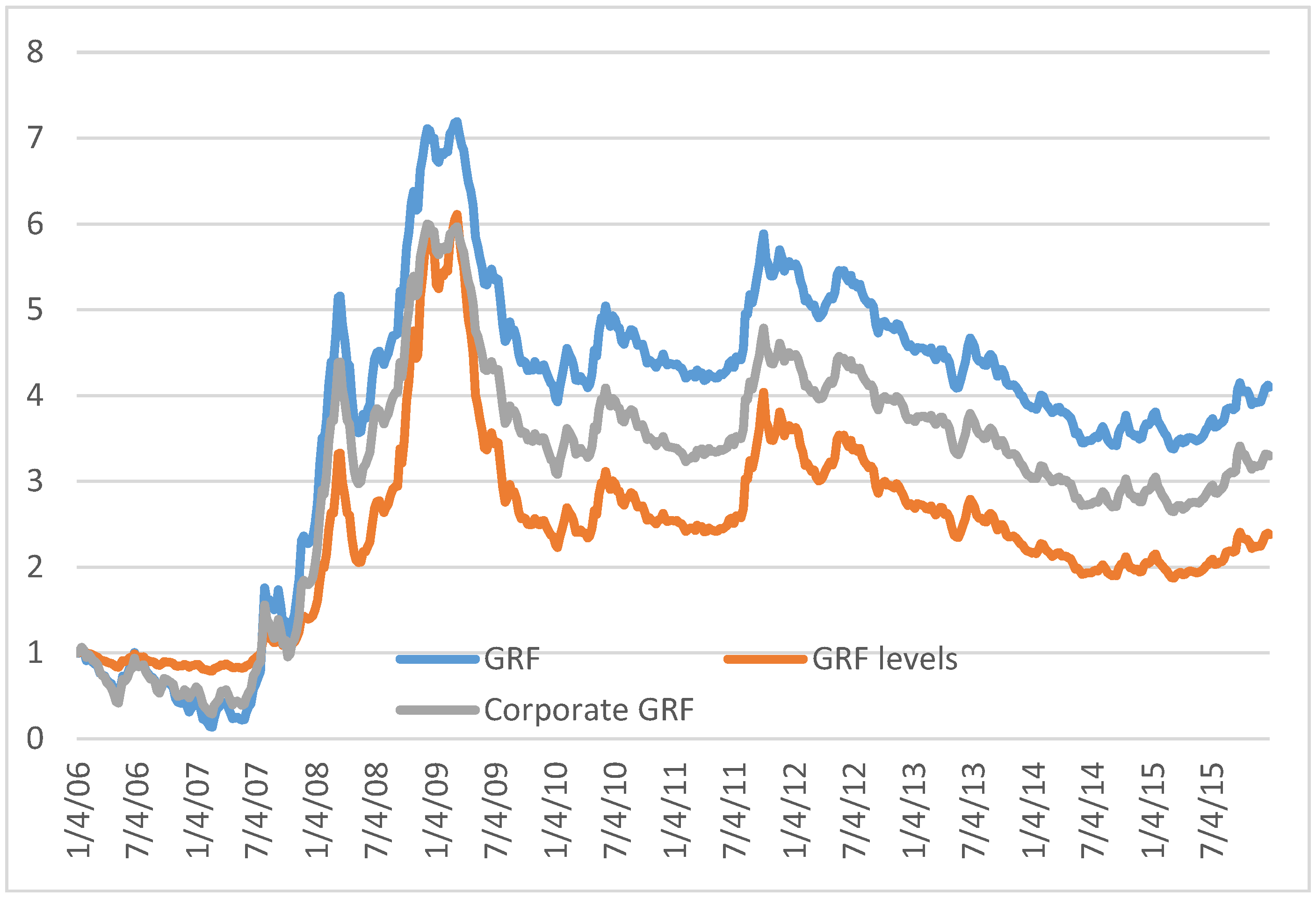
| Risk Indicator | GRF | GRFlevels | Corp GRF |
|---|---|---|---|
| GRF | 1 | 0.986 | 0.908 |
| GRFlevels | 1 | 0.913 | |
| Corp GRF | 1 |
| Sector | GRF | GRFlevels | Corp GRF |
|---|---|---|---|
| BM | 0.70 | 0.67 | 0.70 |
| CG | 0.75 | 0.73 | 0.76 |
| CS | 0.66 | 0.64 | 0.66 |
| EN | 0.63 | 0.60 | 0.62 |
| FIN | 0.71 | 0.68 | 0.70 |
| GOV | 0.64 | 0.63 | 0.64 |
| HC | 0.37 | 0.35 | 0.38 |
| IND | 0.80 | 0.75 | 0.79 |
| TEC | 0.46 | 0.45 | 0.47 |
| TEL | 0.67 | 0.66 | 0.67 |
| UTI | 0.67 | 0.63 | 0.66 |
| Median | 0.67 | 0.64 | 0.66 |
| Sector | Systemic | Idiosyncratic |
|---|---|---|
| US Industrial | 0.997 | 0.942 |
| Europe Industrial | 0.995 | 0.993 |
| US Financial | 0.996 | 0.981 |
| Europe Financial | 0.988 | 0.982 |
| Panel a | |||||
| US | 1y Swap | 5y Swap | 10y Swap | 5y Bond | 10y Bond |
| 1y swap | 1 | 0.66 | 0.49 | 0.58 | 0.44 |
| 5y swap | 0.66 | 1 | 0.94 | 0.95 | 0.89 |
| 10y swap | 0.90 | 0.95 | |||
| 5y bond | 0.90 | ||||
| Europe | 1y swap | 5y swap | 10y swap | 5y bond | 10y bond |
| 1y swap | 1 | 0.72 | 0.51 | 0.63 | 0.45 |
| 5y swap | 1 | 0.91 | 0.91 | 0.83 | |
| 10y swap | 1 | 0.85 | 0.91 | ||
| 5y bond | 1 | 0.89 | |||
| 10y bond | 1 | ||||
| Japan | 1y swap | 5y swap | 10y swap | ||
| 1y swap | 1 | 0.69 | 0.46 | ||
| 5y swap | 0.69 | 1 | 0.89 | ||
| 10y swap | 0.44 | 0.83 | 0.90 | ||
| Panel b | |||||
| Variable | (US, Europe) | (US, Japan) | (Europe, Japan) | Variables | (US, Europe) |
| 10 year bond | 0.76 | 0.55 | 0.56 | 3-month rates | 0.52 |
| 1 year swap | 0.58 | 0.37 | 0.39 | Term structure slopes | 0.60 |
| 5 year swap | 0.68 | 0.50 | 0.53 | VIX, VSTOXX | 0.87 |
| 10 year swap | 0.70 | 0.54 | 0.55 | ViTraxx, VCDX | 0.67 |
| Risk Component | MSCI | Risk Aversion | Macro | Financial |
|---|---|---|---|---|
| European Industrial | ||||
| Systemic | 0.27 | 0.55 | 0.26 | −0.22 |
| Sectorial | 0.40 | 0.50 | 0.53 | −0.54 |
| Idiosyncratic | −0.36 | −0.63 | −0.41 | 0.38 |
| US Industrial | ||||
| Systemic | 0.63 | 0.57 | 0.01 | −0.28 |
| Sectorial | 0.51 | 0.50 | 0.24 | −0.27 |
| Idiosyncratic | −0.64 | −0.60 | −0.11 | 0.31 |
| European Financial | ||||
| Systemic | 0.64 | 0.63 | 0.39 | 0.12 |
| Sectorial | 0.21 | 0.71 | 0.90 | 0.16 |
| Idiosyncratic | −0.48 | −0.81 | −0.80 | −0.18 |
| US Financial | ||||
| Systemic | 0.64 | 0.38 | 0.17 | 0.04 |
| Sectorial | 0.60 | 0.62 | 0.74 | 0.46 |
| Idiosyncratic | −0.78 | −0.59 | −0.49 | −0.26 |
© 2019 by the authors. Licensee MDPI, Basel, Switzerland. This article is an open access article distributed under the terms and conditions of the Creative Commons Attribution (CC BY) license (http://creativecommons.org/licenses/by/4.0/).
Share and Cite
Novales, A.; Chamizo, A. Splitting Credit Risk into Systemic, Sectorial and Idiosyncratic Components. J. Risk Financial Manag. 2019, 12, 129. https://doi.org/10.3390/jrfm12030129
Novales A, Chamizo A. Splitting Credit Risk into Systemic, Sectorial and Idiosyncratic Components. Journal of Risk and Financial Management. 2019; 12(3):129. https://doi.org/10.3390/jrfm12030129
Chicago/Turabian StyleNovales, Alfonso, and Alvaro Chamizo. 2019. "Splitting Credit Risk into Systemic, Sectorial and Idiosyncratic Components" Journal of Risk and Financial Management 12, no. 3: 129. https://doi.org/10.3390/jrfm12030129
APA StyleNovales, A., & Chamizo, A. (2019). Splitting Credit Risk into Systemic, Sectorial and Idiosyncratic Components. Journal of Risk and Financial Management, 12(3), 129. https://doi.org/10.3390/jrfm12030129