Article

Can We Forecast Daily Oil Futures Prices? Experimental Evidence from Convolutional Neural Networks

1
Graduate School of System Informatics, Kobe University, 2-1 Rokkodai, Nada-Ku, Kobe 657-8501, Japan
2
Graduate School of Economics, Kobe University, 2-1 Rokkodai, Nada-Ku, Kobe 657-8501, Japan
*
Author to whom correspondence should be addressed.
J. Risk Financial Manag. 2019, 12(1), 9; https://doi.org/10.3390/jrfm12010009
Submission received: 21 November 2018 / Revised: 25 December 2018 / Accepted: 2 January 2019 / Published: 8 January 2019
(This article belongs to the Special Issue Empirical Finance)

Abstract

:
This paper proposes a novel approach, based on convolutional neural network (CNN) models, that forecasts the short-term crude oil futures prices with good performance. In our study, we confirm that artificial intelligence (AI)-based deep-learning approaches can provide more accurate forecasts of short-term oil prices than those of the benchmark Naive Forecast (NF) model. We also provide strong evidence that CNN models with matrix inputs are better at short-term prediction than neural network (NN) models with single-vector input, which indicates that strengthening the dependence of inputs and providing more useful information can improve short-term forecasting performance.

Graphical Abstract

1. Introduction

Crude oil is a vital fuel, accounting for 32.9% of global energy consumption in 2016 according to BP’s Statistical Energy Outlook, which indicates that crude oil will continue to play an important role until 2035. It is fair to argue that the movement in the crude oil price should have a significant effect on macroeconomic aggregates, such as the GDP and inflation of oil-exporting and -importing countries. On the other hand, as one of the most actively traded commodities in the world (Alvarez-Ramirez et al. (2012)), crude oil futures have become an important financial asset and an additional investment tool. Owing to the increasing correlation between traditional financial markets, such as stocks, bonds, and foreign exchange, international investors are searching for new investment tools, such as crude oil futures, to enhance returns, diversify portfolios, and hedge against inflation. Therefore, forecasting oil futures prices accurately is crucial and helps international investors to diversify risk.
Many researchers have proposed and developed economic models to forecast crude oil spot prices (De Souza e Silva et al. (2010); Ye et al. (2006); Merino and Ortiz (2005); Wang et al. (2016); Wen et al. (2016); Baumeister et al. (2015); Naser (2016)). However, studies forecasting futures prices are scarce. According to Sklibosios Nikitopoulos et al. (2017), futures prices depend on the value of deferred use. For example, decreasing futures prices show that the value of immediate use (consumption) or the yield to holders of physical inventory is reducing. Therefore, futures prices are vulnerable to many complex natural, economic, and political factors, such as the economic development conditions of oil giants, oil wars, international petroleum organizations and so on. A large number of these factors are random, resulting in sharp fluctuations in the crude oil futures markets and showing very complex nonlinear characteristics. Thus, it is difficult to predict the futures prices accurately.
Recently, as new technologies are developed, artificial intelligence (AI) techniques (e.g., neural networks (NNs)) have been applied to the prediction of time series. AI-based models emulate the human brain to provide feedback on large quantities of data, and to learn to recognize information patterns. Thus, NN models can create a breakthrough opportunity in the analysis of the non-linear behavior of the time series of the crude oil markets (Refenes (1994); Ongkrutaraksa (1995); Moshiri and Foroutan (2006); Jammazi and Aloui (2012); Mingming and Jinliang (2012); Wang et al. (2005)). For example, Moshiri and Foroutan (2006) compared linear (Autoregressive moving average models and Generalized autoregressive conditional heteroscedasticity models) and nonlinear NN models, and found that NNs are superior and produce a more statistically significant forecast. Jammazi and Aloui (2012) combined the wavelet transform and NNs to forecast the crude oil monthly price. Mingming and Jinliang (2012) constructed a multiple-wavelet recurrent NN model to analyze crude oil monthly prices. Wang et al. (2005) present an NN-based model to forecast crude oil monthly prices, and claimed superior performance by their model. These results prove that an AI-based forecasting model can provide greater efficiency and higher accuracy than other models.
Here, we propose a novel, deep-learning forecasting approach based on a convolutional neural networks (CNNs) model for short-term1 forecasting using daily data of crude oil futures prices. Unlike NNs with a single-vector neuron, the layers of the CNN model have neurons arranged in two dimensions (width and height). The CNNs take advantage of the fact that the inputs consist of matrices, which can strengthen the dependence and connections between neurons and constrain the architecture in a more sensible way. Moreover, instead of all the neurons in NNs being fully connected, the neurons of the CNN in a layer are only connected to a small region of the previous layer, which enables CNN models to share connections among neurons more flexibly. These characteristics may improve the short-term forecasting of crude oil prices. CNNs have recently been applied to large-scale image and video recognition (Krizhevsky et al. (2012); Zeiler and Fergus (2014); Simonyan and Zisserman (2014)) and traffic-speed prediction (Ma et al. (2017)). To the best of our knowledge, our study is the first CNN approach applied in the economic and financial field, and particularly to crude oil futures prices forecasting. CNN models are used in modeling problems related to spatial inputs like images. They are not suitable for processing and predicting events at relatively long intervals and delays in the time series. However, in our forecasting task, we used the daily oil prices to predict a short-term future price. Thus, CNN is suitable for this task due to its ability to capture the relevant features from the nearby daily prices in an image (one-week daily prices matrix). In addition, we normalized our data to overcome non-stationary time series and focus on the short-term oil futures prices trends using the daily data. We employ CNN models to forecast crude oil daily prices, which has become possible owing to the large daily data set.
Our study offers two contributions to the literature. First, we confirm that the non-linear deep-learning approaches perform better for short-term forecasting by comparing AI-based deep-learning methods with the naive forecast (NF) and Autoregressive-Generalized autoregressive conditional heteroscedasticity (AR-GARCH) model as two benchmarks, in terms of the accuracy of the short-term crude oil price forecasting. Second, we find that strengthening the dependence of inputs and providing more useful information connections between neurons can improve the short-term forecasting performance. Here we show that the CNN models are more powerful than the benchmark models.
The remainder of this paper is organized as follows. In Section 2, we introduce our related work in technology. In Section 3, we describe the model specifications. We show our data and empirical results in Section 4 and Section 5. Finally, our concluding remarks are presented in Section 6.

2. Neural Networks and Convolutional Neural Networks

Neural networks (NNs) are trained on a frame error (FE) minimization criterion, and the corresponding weights are adjusted to minimize the error squares over the whole source-target, stereo training data set. As shown in Equation (1), the mapping error is given by:
ϵ = t | | y t G ( x t ) | | 2 ,
where G ( x t ) denotes the NNs mapping of x t and is defined as:
G ( x t ) = ( G 1 G 2 G L ) = l = 1 L G ( l ) ( x t )
G ( l ) ( x t ) = σ ( W ( l ) x t ) .
Here, l = 1 L denotes a composition of L functions. For instance, l = 1 2 G ( l ) ( x t ) = σ ( W ( 2 ) σ ( W ( 1 ) ( x t ) ) . W ( l ) represents the weight matrix of layer l in the NNs. σ denotes an activation function sigmoid, which has the mathematical form σ ( x ) = 1 / ( 1 + e x ) .
CNNs typically have a standard structure in which the basic design is prevalent in the image (matrix) classification. In recent years, CNNs have been applied in many fields owing to their advanced detection and classification performance (LeCun et al. (1989)). CNNs consist of a sequence of layers. The typical layers in CNNs are: the convolutional layer, pooling layer, and fully-connected layer.
Convolutional layer: As with NNs, CNNs also are made up of neurons with learnable weights Please confirm meaning is retained. and biases, where each neuron receives inputs and performs a dot product, after which the output is computed through non-linearity functions, and called the activation function. However, neurons in the convolutional layer are arranged in 3 dimensions, and they are only connected to small local regions of the previous layer, instead of all outputs. The output of regions is patched out by multiple filters, called convolutional filters. When one convolutional filter W l r is applied to the input, the output can be formulated as:
y c o n v = e = 1 m f = 1 n ( W l r ) e f d e f ,
where m and n are two dimensions of the filter, d e f is the data value of the input matrix at positions e and f, ( W l r ) e f is the coefficient of the convolutional filter at positions e and f, and y c o n v is the output. In the convolutional layers, each filter comprises a local path from lower-level into higher-level features.
Pooling layer: Down sampling is performed in the pooling layer to compress the size of representation. This helps in the computation of the network.
Fully-connected layer: Similar to ordinary NNs, all outputs neurons of previous layers are collected to each neuron in the layer, computing the class scores by linear classifiers, such as SVM and Softmax.
Even though the overall network remains as a single, differentiable score function, as with NNs, CNNs are proven to be more effective with two-dimensional input, such as a matrix, since CNN architectures enable the encoding of certain properties into the architecture by taking advantage of the input structure.

3. Model Design

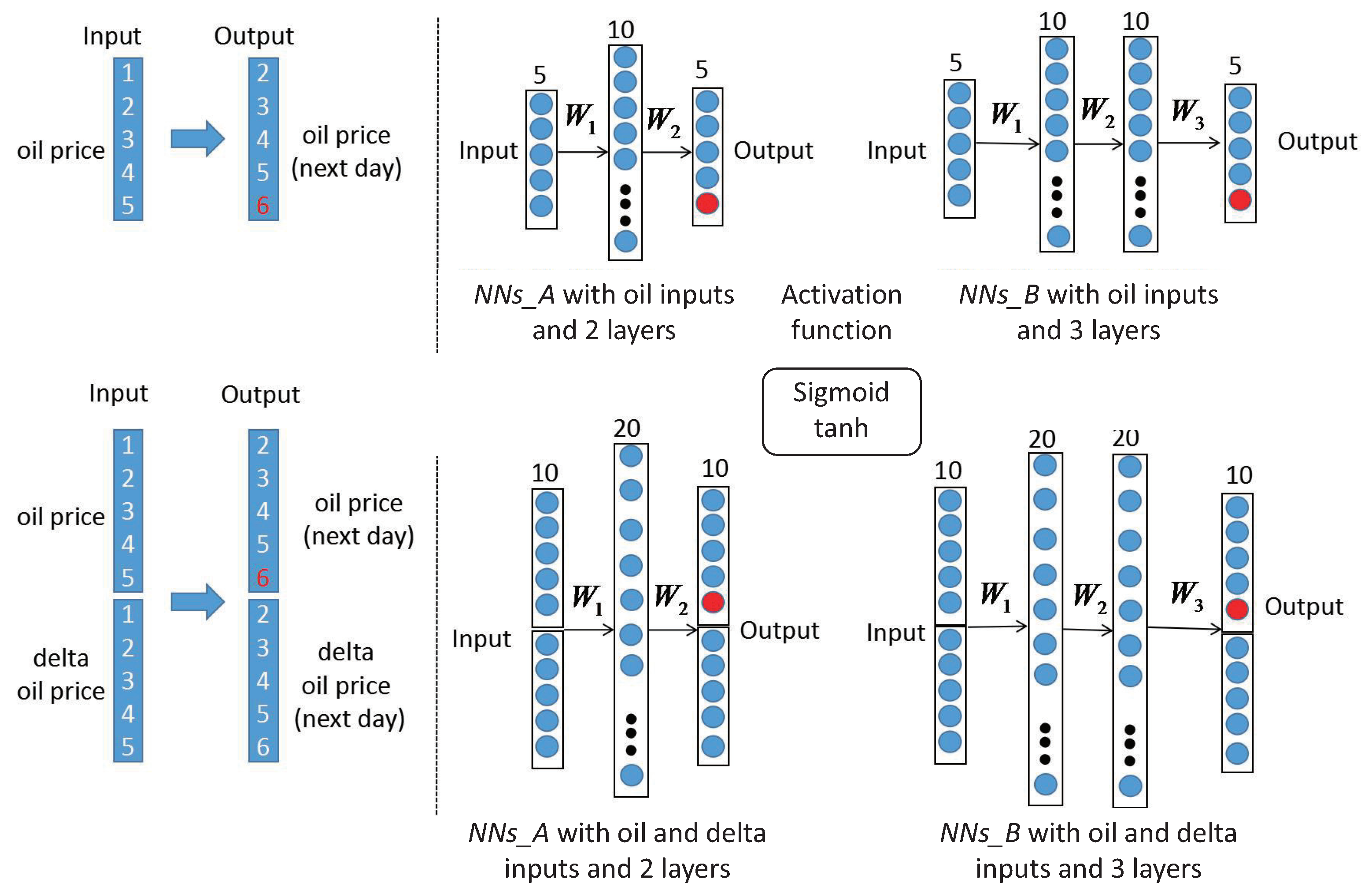
3.1. Method 1: Neural Networks

The methodology formulation of NNs is described in Section 2. In this section, we introduce the NN architecture used to predict the oil price and the steps of the training process.
(1) Transform a sequence of oil prices into segment-level features. We segment a sequence of oil prices by window size w and shift the window by day.
X N = x 1 , , x m , , x N T .
Equation (5) represents N examples of w-dimensional source features, which are composed of daily oil prices input. The daily oil prices of the output are one day after the input daily oil prices. In the proposed model, we set w = 5 , which represents five days of oil price inputs. To guarantee the coordination between the initial input and output features, we adopt the same approach for the target features composed of the daily oil price output, that is, a day after input.
(2) After transforming one-dimensional features to five-dimensional features, we train them using different NNs with different parameters as shown in Figure 1. As shown in the left part of the figure, there are two kinds of input and output data sets: five days’ oil prices and a combination of five days’ oil prices and their delta values. The target output is the input’s next days’ oil prices. The right part of the figure shows four different architecture NNs. The top left model N N s _ A uses the two-layer NNs model to train the oil prices. The number of nodes from the input layer x to the output layer are [5, 10, 5]. The top right model N N s _ B uses the three layers with the nodes [5, 10, 10, 5]. The bottom model N N s _ A and N N s _ B use oil prices and their delta values as the input and output, N N s _ A uses the two layers with the nodes [10, 20, 10], and N N s _ B uses the three layers with the nodes [10, 20, 20, 10]. Every model is trained with sigmoid and tanh activation functions, respectively. As shown in the training model, W 1 , W 2 , and W 3 represent the weight matrix of the first, second, and third layers of NNs, respectively. In this paper, we train the oil prices from start to N 100 (N denotes sample size) and we test the last 100 days of oil prices. The results are introduced in the experiment section.

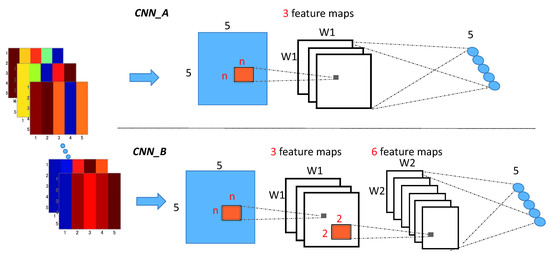
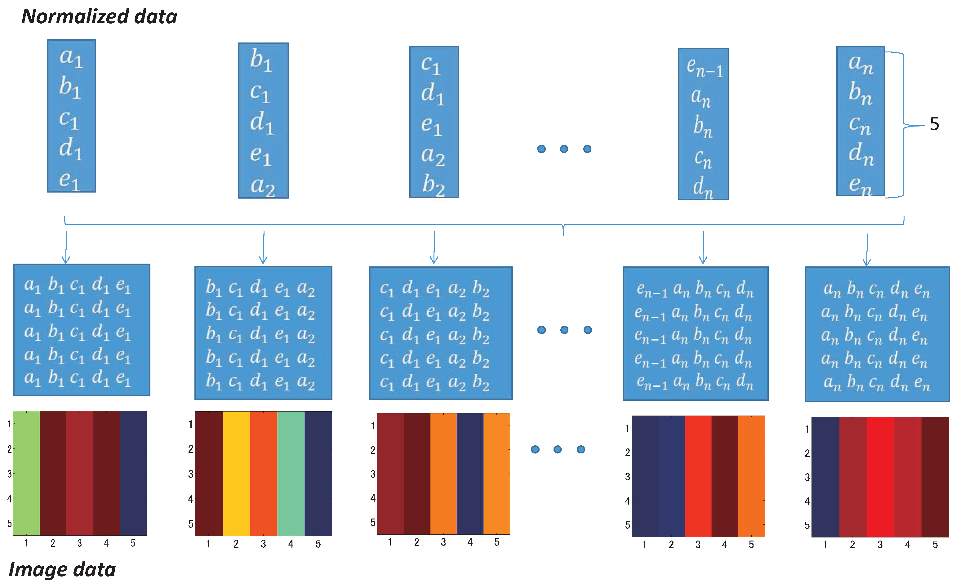
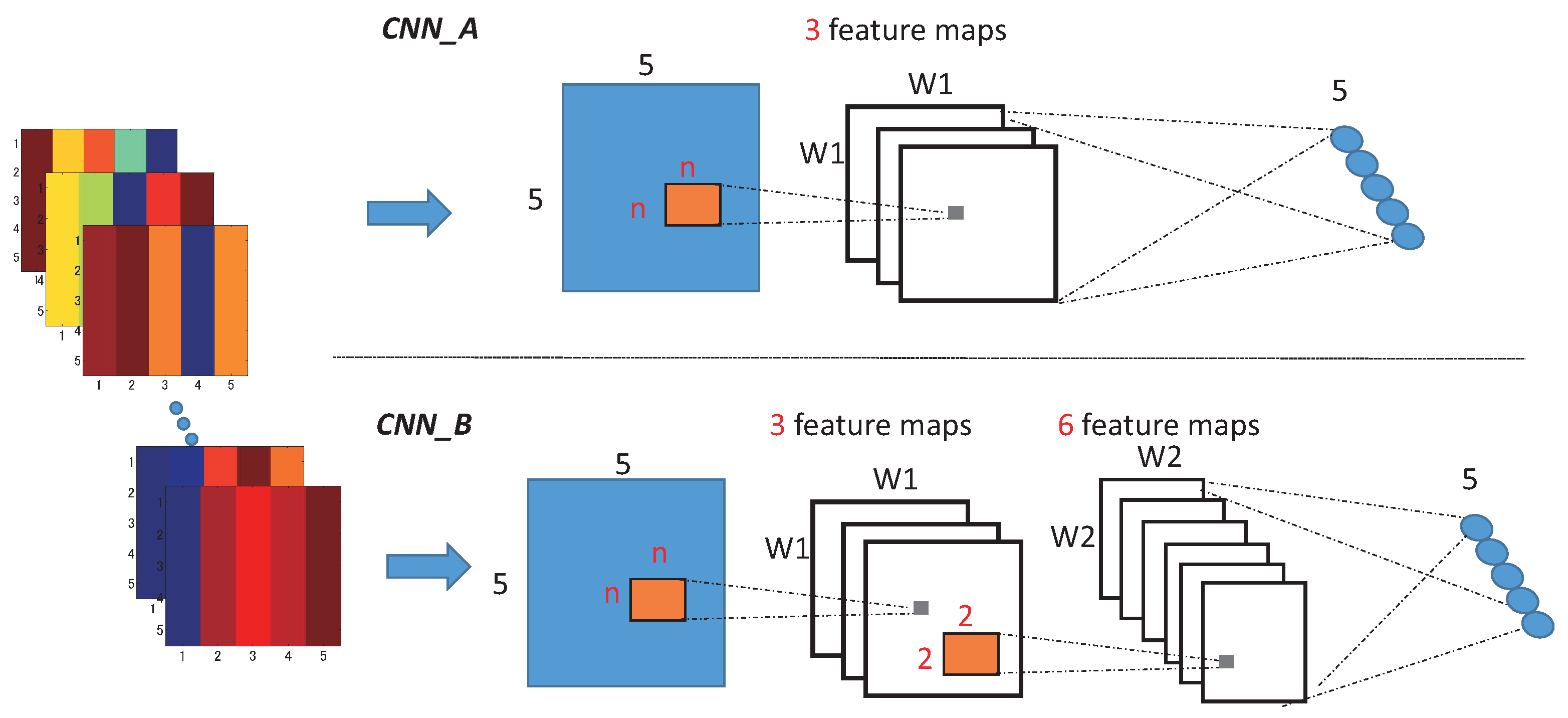
3.2. Method 2: Convolutional Neural Networks

The basic model of a convolutional neural network is described in Section 2. In this section, we describe how to translate the data to the matrix. Then, the architectures used for predicting the oil price are introduced. Since the image is small, we do not apply a pooling layer in this paper.
(1) Transform the sequence of oil prices into a matrix suitable for CNN training. As shown in Figure 2, a, b, c, d, and e represent normalized oil values in Monday, Tuesday, Wednesday, Thursday, and Friday, respectively. For example, a 1 - e 1 represent the prices from Monday to Friday of the first week, and a n - e n represent the prices from Monday to Friday of the n-th week. We copy each week’s oil prices five times and transform them to 5 × 5-size images, where the colors represent different oil prices.
(2) An overview of our CNN architectures is depicted in Figure 3. We train the two CNN architectures with different parameters using the data. As shown in the figure, C N N _ A net contains two layers with weight; the first is convolutional and the second is fully-connected layers. C N N _ B net contains three layers with weights; the first two are convolutional and the last is a fully-connected layer. The outputs of the last fully-connected layer are all fed to a five-way2 Softmax, which produces the predicted oil values over the true values. The kernels of all convolutional layers are connected to the previous layer, and neurons in the fully-connected layers are connected to all neurons. The two models are trained with sigmoid and tanh activation functions, respectively. For the two models, the first convolutional layer filters the 5 × 5 image with the three kernels of size n × n with a stride of one pixel. The stride is the distance between the receptive field centers of neighboring neurons in a kernel map, and we set the stride of the filters to one pixel for all the other layers. For comparison, n will be set to 2 and 3 in the experiment section. In C N N _ A , the output of the first convolutional layer is the input of the C N N _ A ’s last fully-connected layer. In C N N _ B , the output of the first convolutional layer is the input of C N N _ B ’s second convolutional layer, and the second convolutional layer filters the input with six kernels of size 2 × 2 × 3. The output of the second convolutional layer is the input of the C N N _ B ’s last fully-connected layer. The image size of each layer is calculated as follows:
W 1 = ( W n + 2 P ) / S , W 2 = ( W 2 + 2 P ) / S
W is the input image size. S is the stride with which we slide the filter. When the stride is 1, we move the filters one pixel at a time. When the stride is 2, then the filters jump two pixels at a time as we slide them around. P represents the zero-padding, which pads the input volume with zeros around the border. As described above, n is the kernel size. In this case, the input image is 5 × 5, so W is 5, the stride S is set to 1, and no zero-padding is P = 0 . W 1 and W 2 represent the image size after the convolutional processing. When training the CNN models, we used the Adam optimizer Kingma and Ba (2014) with a mini-batch size of 20. The learning rate was set to 0.01, and the momentum term was set to 0.1.

4. Data

In this study, we use the daily Brent crude oil generic series of the first month’s futures prices, traded on the Intercontinental Exchange (ICE). The data cover the period from 24 June 1988, to 3 November 2018, consisting of 7942 observations. The data were obtained from Bloomberg.
For training neural networks, data normalization is an effective way to obtain better performance and quick convergence. Usually, we subtract the mean value to make the input mean zero to prevent weights changing in the same directions, which is called the zero-mean normalization method.
The values of attribute X are normalized using the mean and standard deviation of X. A new value X n is obtained using the following expression:
X n = ( X U x ) S x ,
where U x and S x are the mean and standard deviation of attribute X, respectively. If U x and S x are not known, they can be estimated from the samples. After zero-mean normalizing, each feature will have a mean value of 0. In addition, the unit of each value will be the number of (estimated) standard deviations away from the (estimated) mean. When zero-mean normalization is applied, all data in each profile are slid vertically so that their average is zero. In most neural networks, they normalize the data by the mean of all data. As shown in Figure 4, the middle curve is obtained from the top one by a vertical translation so that the average of the profile is zero. Our method draws its strength from making normalization a part of the model architecture and performing the normalization for different training segmentation using the following formula:
n = N u m l ( X ) / k
X s i = ( X i U i ) S i , i = 1 , 2 , 3 , . . . , n .
Here, N u m l ( X ) represents the sample size of the attribute X. k is the scale of segmentation days, and denotes how many days are concluded in one batch for normalization. For instance, if we set k to 100, it means using the mean value and standard deviations calculated in each 100-day period for normalization. n is the batch number in normalization, and U i and S i are the mean and standard deviation, respectively, of each segmentation attribute X i . X s i is the new normalized value obtained from each batch. As shown in Figure 4, the bottom curve represents the normalized value for k = 20 . Different batch sizes used in normalization lead to different results in the training part. We describe the results in the experiment section.

5. Empirical Results

5.1. Evaluation Criteria

To evaluate the forecasting performance, we calculate the directional accuracy (DA), the root mean absolute error (RMAE), and Theil’s U between the actual values and predicted values, which are often used in the literature (Jammazi and Aloui (2012); Drachal (2016); Yu et al. (2017); Zhao et al. (2017)).
The DA can represent the directional accuracy of each day between the actual data and predicted data, which can be expressed as follows:
D A = 1 N t = 1 N Z t , t = 1 , 2 , . . . , N
Z t = 1 ( V t a V t 1 a ) ( V t p V t 1 p ) 0 0 o t h e r w i s e
where V t a and V t p denote the actual value and predicted value, respectively. N represents the number of days in the testing data. A lower RMAE means a smaller difference between the actual value and predicted value, while a lager DA represents a higher directional accuracy of the predicted value.
The RMAE can reflect the disparity between the actual values and predicted values, which is as follows:
R M A E = 1 N t = 1 N V t a V t p
Thus, a higher value of DA and a lower RMAE represent the better forecasting performance of the model.
We also calculate the Theil’s U to compare the forecast performance of different models with benchmark models.
U = t = 1 N ( V t + 1 p V t + 1 a V t a ) 2 t = 1 N ( V t + 1 a V t a V t a ) 2
If U = 1 , that means the proposed model forecast with an accuracy equal to that of the benchmark-NF model. If U > 1 , that implies the NF model offers a better forecast performance than the proposed model. And if U < 1 , that means the proposed model provides evidence of a better forecasting performance.
Moreover, we use the Diebold-Mariano (DM) test to investigate whether two competing forecasts have equal predictive accuracy. According to Diebold and Mariano (1995), we first define the forecast errors as:
e i t = y ^ i t y i t , i = 1 , 2 t = 1 , 2 , . . . , N
The loss associated with forecast i is assumed to be a function of the forecast error e i t , and is denoted by g ( e i t ) = e i t 2 in this paper. We then define the loss differential between the two forecasts by:
d t = g ( e 1 t ) g ( e 2 t )
The null hypothesis is H 0 : E ( d t ) = 0 , meaning that the forecasts of two different models have the same accuracy while the alternative hypothesis H 1 : E ( d t ) 0 is that they have different levels of forecast accuracy. Finally, we define the Diebold-Mariano statistics as
D M = d ¯ 1 N × s
where d ¯ = 1 N × t = 1 N ( d t ) , s denotes the variance of d t . If DM is positive, that means the forecast errors of the second model are smaller than the first model. Under the null hypothesis, the test statistics DM is asymptotically N ( 0 , 1 ) distributed.

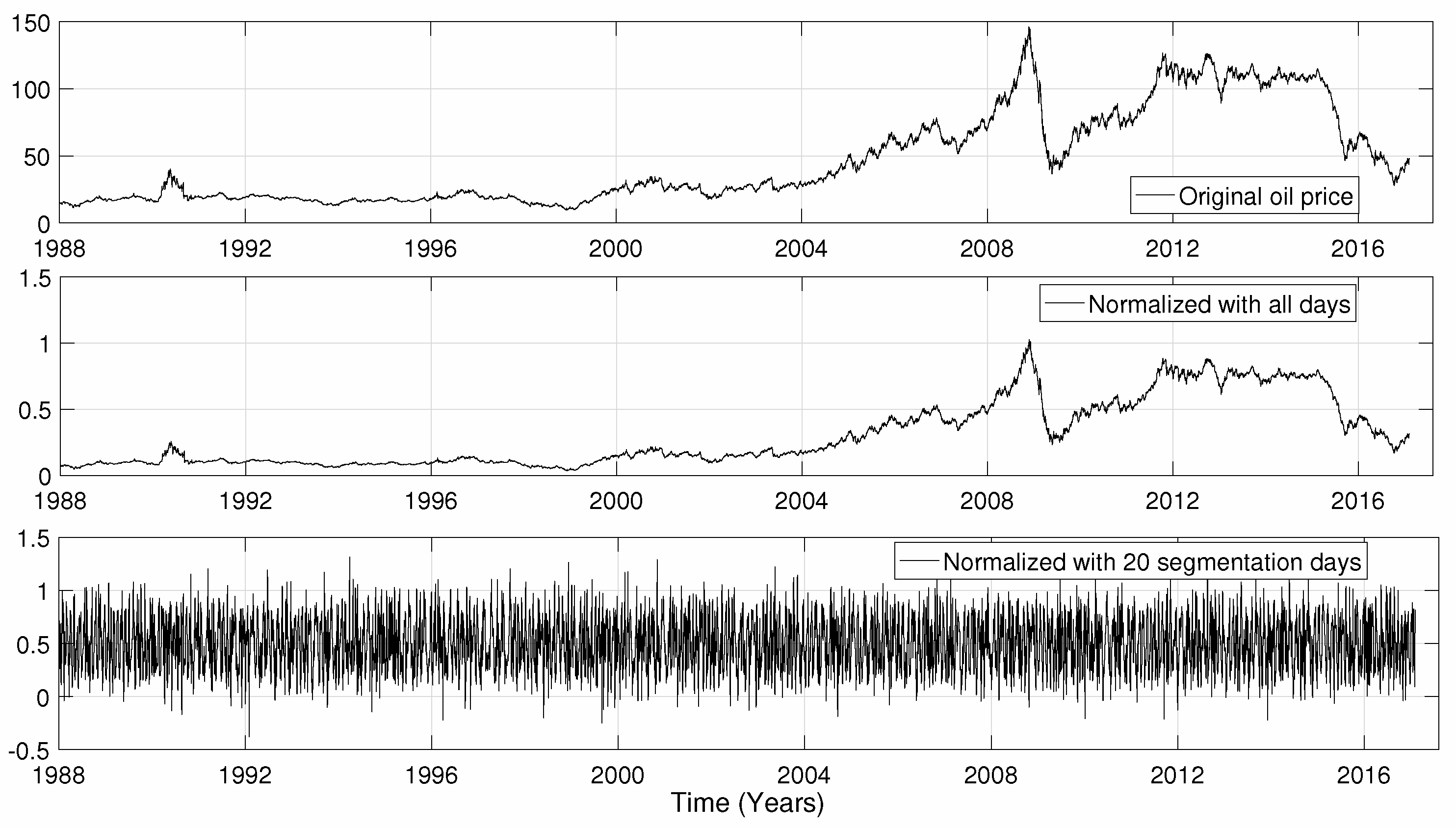
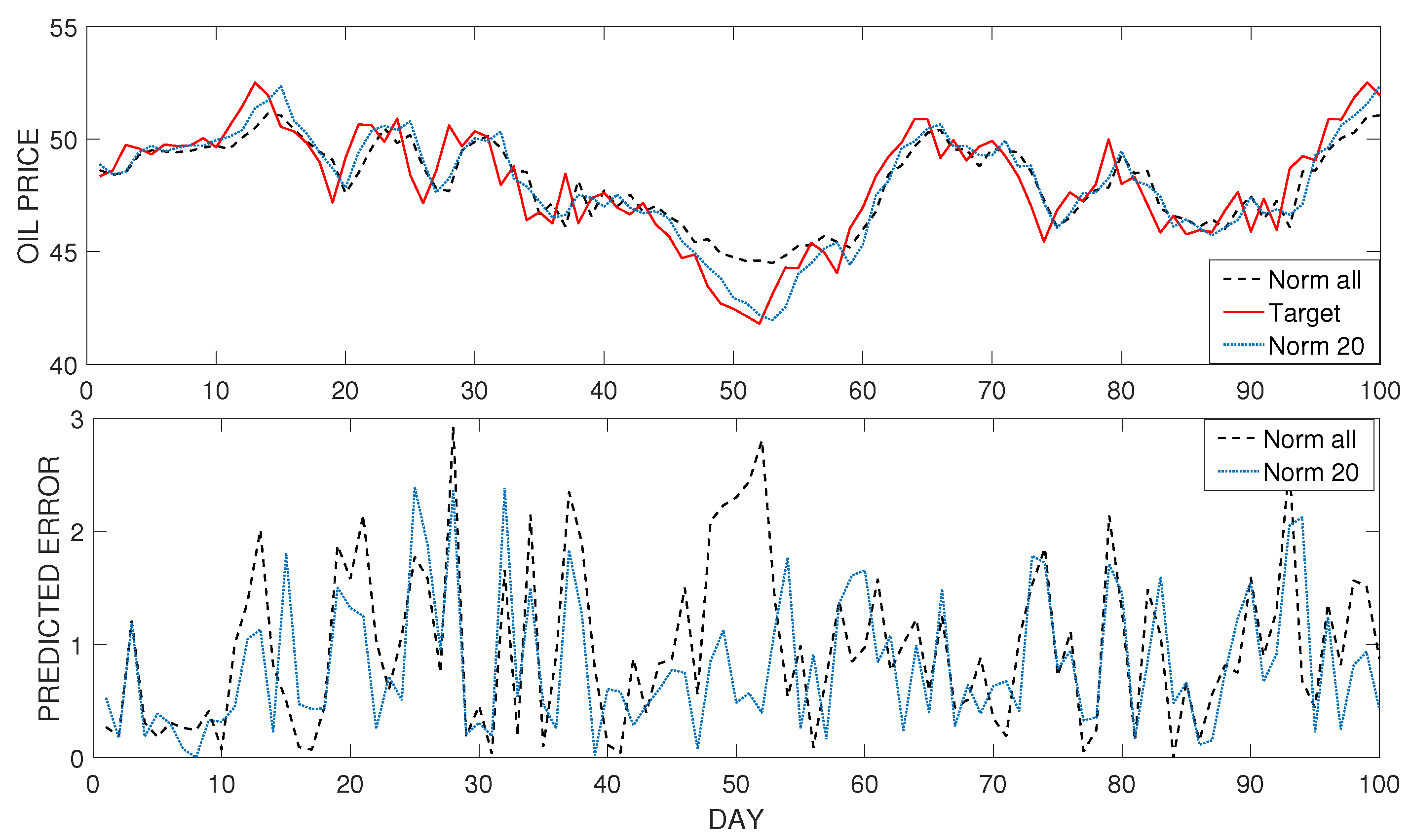
5.2. Normalization Influence

In this section, we test the last 100-day oil price forecasting using the NN model and the two types of normalization methods described in Section 3.1 and Section 4. We report the results in Figure 5. As shown in the top portion of Figure 5, the red curve represents the actual oil prices in the testing part. The black curve represents the predicted oil prices that are calculated by the normalization method using all sample data. The blue one represents the predicted price calculated by the segmentation normalization method of every 20-day period as a batch. The bottom portion of Figure 5 shows the predicted error of the two segmentation normalization methods. We can intuitively see that the latter normalization method can achieve a lower predicted error, which means a better forecasting performance. Thus, we use the 20-day period as a batch to normalize the input data in the training model for short-term oil price forecasting.

5.3. Results

In this subsection, the empirical results of NNs and CNNs are given. For each model, different kinds of activation functions, inputs, and layers will be set for comparison. Table 1 shows the forecasting performance of the NF, AR-GARCH, and NN models. In the NF model, the oil price tomorrow is set equal to today’s price and the probability of an increase (decrease) in the price next day is 50%. From Table 1, we can see that all NN models achieve larger DA and smaller RMAE values than the NF and AR-GARCH models, confirming that the AI-based forecasting model can provide greater efficiency and higher accuracy. As shown in Table 1, N N s _ A denotes the two-layer NN model without and with the delta values of oil prices, while N N s _ B represents the three-layer NN model without and with the delta values. We find that most N N s _ B with two and three layers of different activation functions show a better forecasting performance than those of N N s _ A , implying that the model with deep layers provides higher accuracy of forecasting than the shallow architecture model. The result is in line with Bengio (2009). The three-layer NN model N N s _ B can obtain the largest DA values by using the sigmoid activation function and achieves the smallest RMAE values by using the tanh activation function. Moreover, we also find that the Theil’s U value of AR-GARCH is very close to 1, implying that the forecast accuracy of AR-GARCH is equal with the benchmark of the NF model, while all Theil’s U values of NN models are less than 1, which means NN models offer better forecasting performances than NF and AR-GARCH models.
Table 2 shows the results of the NF, AR-GARCH, and our proposed CNN models with different parameters, where C N N _ A and C N N _ B represent two-layer and three-layer CNN models, respectively. For each model, we set two kernel sizes-2 × 2 and 3 × 3. As shown in Table 2, we find that all CNN models have larger DA and smaller RMAE and Theil’s U values than the NF and AR-GARCH models, which suggests that the deep-learning model can provide higher accuracy for short-term forecasting. This result is consistent with Table 1. In addition, by comparing the CNN with NN models with the same activation functions and layers, we can see that most of the DA (RMAE) values of the CNN models are larger (smaller) than those of NN models, providing strong evidence that CNN models with matrix inputs have better short-term prediction performance than the NN models with single-vector input. We also find that C N N _ A / C N N _ B with 3 × 3 kernel size achieves the higher DA and lower RMAE values than C N N _ A / C N N _ B with 2 × 2 kernel size, suggesting that the large kernel size works on the short-term forecasting performance. In addition, we find that the CNN models with the sigmoid function obtain the lower RMAE values while the higher DA values occur in the CNN models with the tanh function.
We also forecast the crude oil prices during two different sub-periods, including the pre-crisis period (24 June 1988–15 September 2008) and the post-crisis period (14 September 2009–3 December 2018) to test the robustness of our CNN models. The empirical results are shown in Table 3 and Table 4. Similarly, the proposed CNN models have higher DA and smaller RMAE and Theil’s U values than the NF and AR-GARCH models during both two sub-periods. Specifically, C N N _ B with 3 × 3 kernel size offers the best forecast performance.
Table 5 shows the results of the DM test in terms of the statistics and p-values. According to the statistic values, we find most values are positive, meaning that the second model gives smaller forecast errors than the first one. According to the results of the DM test, it can be found that in most cases the difference in forecasting performance seems significant, with a confidence level of 99%. The results provide evidence that the compared two forecasts have different levels of accuracy.

6. Conclusions

As one of the major drivers of the global economy, the crude oil price fluctuation affects the real economy worldwide. Specifically, the importance of the oil futures markets as a common investment alternative to traditional markets has increased. Thus, forecasting oil futures prices accurately can provide useful information that helps international investors to diversify risk. However, the prices of crude oil are influenced by many complex natural, economic, and political factors, which cause the crude oil futures prices show very complex nonlinear characteristics. Thus, it is very hard to predict the prices of crude oil accurately by using the traditional economic models. The evolution of a good forecasting model for oil prices is of great importance.
In this study, we develop a new forecasting methodology based on CNNs to forecast the short-term crude oil futures prices. We first compare the AI-based deep-learning model with the benchmark models. We then employ the CNN model with matrix inputs for short-term prediction. In our paper, we confirm that the non-linear AI-based deep-learning approach can provide higher accuracy than the benchmark models. We also find that the CNNs are more powerful than the benchmark models. These results imply that increasing the dependence of inputs and providing more useful information are effective ways of improving the forecasting performance.
References

Author Contributions

Conceptualization: S.H. and T.T.; Formal Analysis: Z.L. and X.C.; Writing—Original draft preparation: Z.L. and X.C.; Writing—Reviewing and editing: K.T., T.T., T.K. and S.H.; Funding Acquisition: T.T. and S.H.

Funding

This work was supported by JSPS KAKENHI Grant Number 17K18564 and (A) 17H00983.

Acknowledgments

We would like to acknowledge the valuable comments from the Reviewers of Journal of Risk and Financial Management.

Conflicts of Interest

The authors declare no conflicts of interest.

References

  1. Alvarez-Ramirez, Jose, Eduardo Rodriguez, Esteban Martina, and Carlos Ibarra-Valdez. 2012. Cyclical behavior of crude oil markets and economic recessions in the period 1986–2010. Technological Forecasting and Social Change 79: 47–58. [Google Scholar] [CrossRef]
  2. Baumeister, Christiane, Pierre Guérin, and Lutz Kilian. 2015. Do high-frequency financial data help forecast oil prices? The MIDAS touch at work. International Journal of Forecasting 31: 238–52. [Google Scholar] [CrossRef]
  3. Bengio, Yoshua. 2009. Learning deep architectures for AI. Foundations and Trends® in Machine Learning 2: 1–127. [Google Scholar] [CrossRef]
  4. De Souza e Silva, Edmundo G., Luiz F.L. Legey, and Edmundo A. de Souza e Silva. 2010. Forecasting oil price trends using wavelets and hidden Markov models. Energy Economics 32: 1507–19. [Google Scholar] [CrossRef]
  5. Diebold, Francis X., and Roberto S. Mariano. 1995. Comparing predictive accuracy. Journal of Business and Economic Statistics 13: 253–63. [Google Scholar]
  6. Drachal, Krzysztof. 2016. Forecasting spot oil price in a dynamic model averaging framework—Have the determinants changed over time? Energy Economics 60: 35–46. [Google Scholar] [CrossRef]
  7. Jammazi, Rania, and Chaker Aloui. 2012. Crude oil price forecasting: Experimental evidence from wavelet decomposition and neural network modeling. Energy Economics 34: 828–41. [Google Scholar] [CrossRef]
  8. Kingma, Diederik P., and Jimmy Ba. 2014. Adam: A method for stochastic optimization. arXiv, arXiv:1412.6980. [Google Scholar]
  9. Krizhevsky, Alex, Ilya Sutskever, and Geoffrey E. Hinton. 2012. Imagenet classification with deep convolutional neural networks. Paper presented at the 25th International Conference on Neural Information Processing Systems, Lake Tahoe, NV, USA, December 3–6; pp. 1097–105. [Google Scholar]
  10. LeCun, Yann, Bernhard E. Boser, John Denker, Don Henderson, Richard E. Howard, Wayne Hubbard, and Larry Jackel. 1989. Backpropagation applied to handwritten zip code recognition. Neural Computation 1: 541–51. [Google Scholar] [CrossRef]
  11. Ma, Xiaolei, Zhuang Dai, Zhengbing He, Jihui Na, Yong Wang, and Yunpeng Wang. 2017. Learning traffic as images: A deep convolutional neural network for large-scale transportation network speed prediction. Sensors 17: 818. [Google Scholar] [CrossRef] [PubMed]
  12. Merino, Antonio, and Álvaro Ortiz. 2005. Explaining the so-called “price premium” in oil markets. OPEC Energy Review 29: 133–52. [Google Scholar] [CrossRef]
  13. Moshiri, Source, and Faezeh Foroutan. 2006. Forecasting nonlinear crude oil futures prices. The Energy Journal 27: 81–95. [Google Scholar] [CrossRef]
  14. Naser, Hanan. 2016. Estimating and forecasting the real prices of crude oil: A data rich model using a dynamic model averaging (DMA) approach. Energy Economics 56: 75–87. [Google Scholar] [CrossRef]
  15. Ongkrutaraksa, Worapot. 1995. Fractal Theory and Neural Networks in Capital Markets. Working Paper at Kent State University. Kent: Kent State University. [Google Scholar]
  16. Refenes, Apostolos Paul. 1994. Neural Networks in the Capital Markets. New York: John Wiley & Sons, Inc. [Google Scholar]
  17. Simonyan, Karen, and Andrew Zisserman. 2014. Two-stream convolutional networks for action recognition in videos. In Advances in Neural Information Processing Systems. Cambridge: MIT Press, pp. 568–76. [Google Scholar]
  18. Sklibosios Nikitopoulos, Christina, Matthew Squires, Susan Thorp, and Danny Yeung. 2017. Determinants of the crude oil futures curve: Inventory, consumption and volatility. Journal of Banking and Finance 84: 53–67. [Google Scholar] [CrossRef]
  19. Tang, Mingming, and Jinliang Zhang. 2012. A multiple adaptive wavelet recurrent neural network model to analyze crude oil prices. Journal of Economics and Business 64: 275–86. [Google Scholar]
  20. Wang, Shouyang, Lean Yu, and Kin Keung Lai. 2005. Crude oil price forecasting with TEI@ I methodology. Journal of Systems Science and Complexity 18: 145–66. [Google Scholar]
  21. Wang, Yudong, Chongfeng Wu, and Li Yang. 2016. Forecasting crude oil market volatility: A Markov switching multifractal volatility approach. International Journal of Forecasting 32: 1–9. [Google Scholar] [CrossRef]
  22. Wen, Fenghua, Xu Gong, and Shenghua Cai. 2016. Forecasting the volatility of crude oil futures using HAR-type models with structural breaks. Energy Economics 59: 400–13. [Google Scholar] [CrossRef]
  23. Yu, Lean, Yang Zhao, and Ling Tang. 2017. Ensemble forecasting for complex time series using sparse representation and neural networks. Journal of Forecasting 36: 122–38. [Google Scholar] [CrossRef]
  24. Ye, Michael, John Zyren, and Joanne Shore. 2006. Forecasting short-run crude oil price using high-and low-inventory variables. Energy Policy 34: 2736–43. [Google Scholar] [CrossRef]
  25. Zeiler, Matthew D., and Rob Fergus. 2014. Visualizing and understanding convolutional networks. Paper presented at the European Conference on Computer Vision, Zurich, Switzerland, September 6–12; pp. 818–33. [Google Scholar]
  26. Zhao, Yang, Jianping Li, and Lean Yu. 2017. A deep learning ensemble approach for crude oil price forecasting. Energy Economics 66: 9–16. [Google Scholar] [CrossRef]
1.
In this paper, the short-term forecast means the next day forecast that is the forecast is 1-step-ahead.
2.
In fact, we also used the 2 and 3 output layers and we find there are not obvious differences among 5 output nodes in forecast performance, which implies the robustness of our CNN models.
Figure 1. Neural network (NN) models with different layers and parameters.
Jrfm 12 00009 g001
Figure 2. Transform data to matrix inputs (a-e denote the normalized oil prices from Monday to Friday, for example a 1 - e 1 represent the prices from Monday to Friday of the first week and a n - e n represent the prices from Monday to Friday of the n-th week).
Jrfm 12 00009 g002
Figure 3. Train the 5 × 5-size economic data images by two different architectures. Convolutional neural network (CNN). C N N _ A (top): two-layers model with one convolutional layer and one fully-connected layer. C N N _ B (bottom): three-layers model with two convolutional layers and one fully-connected layer.
Jrfm 12 00009 g003
Figure 4. The original oil price (top), the normalized oil price by zero-mean normalization with all data (middle), and 20 segmentation days (bottom), respectively.
Jrfm 12 00009 g004
Figure 5. (Top) Target oil price (red) and the predicted price by the normal normalization method (black) and the segmentation normalization method (blue); (Bottom) The predicted error calculated from different normalization methods.
Jrfm 12 00009 g005
Table 1. Directional accuracy (DA), root mean absolute error (RMAE) and Theil’s U results of NN models.
ModelsFunctionsInputsLayersDARMAETheil’s U
NF---0.4950.9091
AR-GARCH---0.4500.9101.000
N N s _ A SigmoidOil20.5360.8160.865
N N s _ B SigmoidOil30.5670.7850.814
N N s _ A SigmoidOil-delta20.5410.8010.832
N N s _ B SigmoidOil-delta30.5750.8080.802
N N s _ A TanhOil20.5140.8350.838
N N s _ B TanhOil30.5570.7930.813
N N s _ A TanhOil-delta20.5450.8110.821
N N s _ B TanhOil-delta30.5560.7760.782
Notes: NF denotes naive forecast. In the NF, the oil price tomorrow is equal to today’s price, and the probability of an increase (decrease) in the price tomorrow is 50%; AR-GARCH denotes the AR(1)-GARCH(1, 1) model; N N s _ A and N N s _ B represent 2-layer NNs models with [5, 10, 5] and 3-layer with the nodes [5, 10, 10, 5], respectively. The numbers in bold represent the best forecast performance.
Table 2. DA, RMAE and Theil’s U results of CNN models (Full sample: 24 June 1988 to 3 December 2018).
ModelsFunctionsInputsKernel SizeLayersDARMAETheil’s U
NF----0.4950.9091
AR-GARCH----0.4500.9101.000
C N N _ A SigmoidOil2 × 220.5230.7320.781
C N N _ B SigmoidOil2 × 230.5420.7450.763
C N N _ A SigmoidOil3 × 320.5350.7280.743
C N N _ B SigmoidOil3 × 330.5500.7410.762
C N N _ A TanhOil2 × 220.5610.7530.776
C N N _ B TanhOil2 × 230.5740.7720.791
C N N _ A TanhOil3 × 320.5950.7390.752
C N N _ B TanhOil3 × 330.5580.7850.755
Notes: NF denotes naive forecast. In the NF, the oil price tomorrow is equal to the today’s price and the probability of an increase (decrease) in the price tomorrow is 50%; AR-GARCH denotes the AR(1)-GARCH(1, 1) model; C N N _ A and C N N _ B represent 3-layer and 4-layer CNN models, respectively. The numbers in bold represent the best forecast performance.
Table 3. DA, RMAE and Theil’s U results of CNN models (Subperiod 1: 24 June 1988 to 15 September 2008).
ModelsFunctionsInputsKernel SizeLayersDARMAETheil’s U
NF----0.4151.3631
AR-GARCH----0.4001.3741.001
C N N _ A SigmoidOil2 × 220.4361.2590.821
C N N _ B SigmoidOil2 × 230.4411.2450.814
C N N _ A SigmoidOil3 × 320.4551.1290.796
C N N _ B SigmoidOil3 × 330.4751.1910.842
C N N _ A TanhOil2 × 220.4831.1620.806
C N N _ B TanhOil2 × 230.4781.2130.829
C N N _ A TanhOil3 × 320.4921.1250.811
C N N _ B TanhOil3 × 330.4591.2570.801
Notes: NF denotes naive forecast. In the NF, the oil price tomorrow is equal to the today’s price and the probability of an increase (decrease) in the price tomorrow is 50%; AR-GARCH denotes the AR(1)-GARCH(1, 1) model; C N N _ A and C N N _ B represent 3-layer and 4-layer CNN models, respectively. The numbers in bold represent the best forecast performance.
Table 4. DA, RMAE and Theil’s U results of CNN models (Subperiod 2: 14 September 2009 to 3 December 2018).
ModelsFunctionInputsKernel SizeLayersDARMAETheil’s U
NF----0.4950.9091
AR-GARCH----0.4900.9101.000
C N N _ A SigmoidOil2 × 220.5050.8910.983
C N N _ B SigmoidOil2 × 230.5170.8630.956
C N N _ A SigmoidOil3 × 320.4950.8510.942
C N N _ B SigmoidOil3 × 330.5230.8650.923
C N N _ A TanhOil2 × 220.4910.8740.996
C N N _ B TanhOil2 × 230.5010.8810.962
C N N _ A TanhOil3 × 320.5250.8840.950
C N N _ B TanhOil3 × 330.5190.7850.956
Notes: NF denotes naive forecast. In the NF, the oil price tomorrow is equal to the today’s price and the probability of an increase (decrease) in the price tomorrow is 50%; AR-GARCH denotes the AR(1)-GARCH(1, 1) model; C N N _ A and C N N _ B represent 3-layer and 4-layer CNN models, respectively. The numbers in bold represent the best forecast performance.
Table 5. Diebold-Mariano (DM) test results.
NF vs. AR-GARCHNF vs. NNNF vs. CNN
Statistics−0.3134.0393.640
P-values0.7550.0000.000
AR-GARCH vs. NNAR-GARCH vs. CNNNN vs. CNN
Statistics4.0353.6352.308
P-values0.0000.0000.023
Notes: NF denotes naive forecast. In the NF, the oil price tomorrow is equal to the today’s price and the probability of an increase (decrease) in the price tomorrow is 50%; AR-GARCH denotes the AR(1)-GARCH(1, 1) model; N N represents the best forecast performance model in NN models; C N N represents the best forecast performance model in our CNN models.

