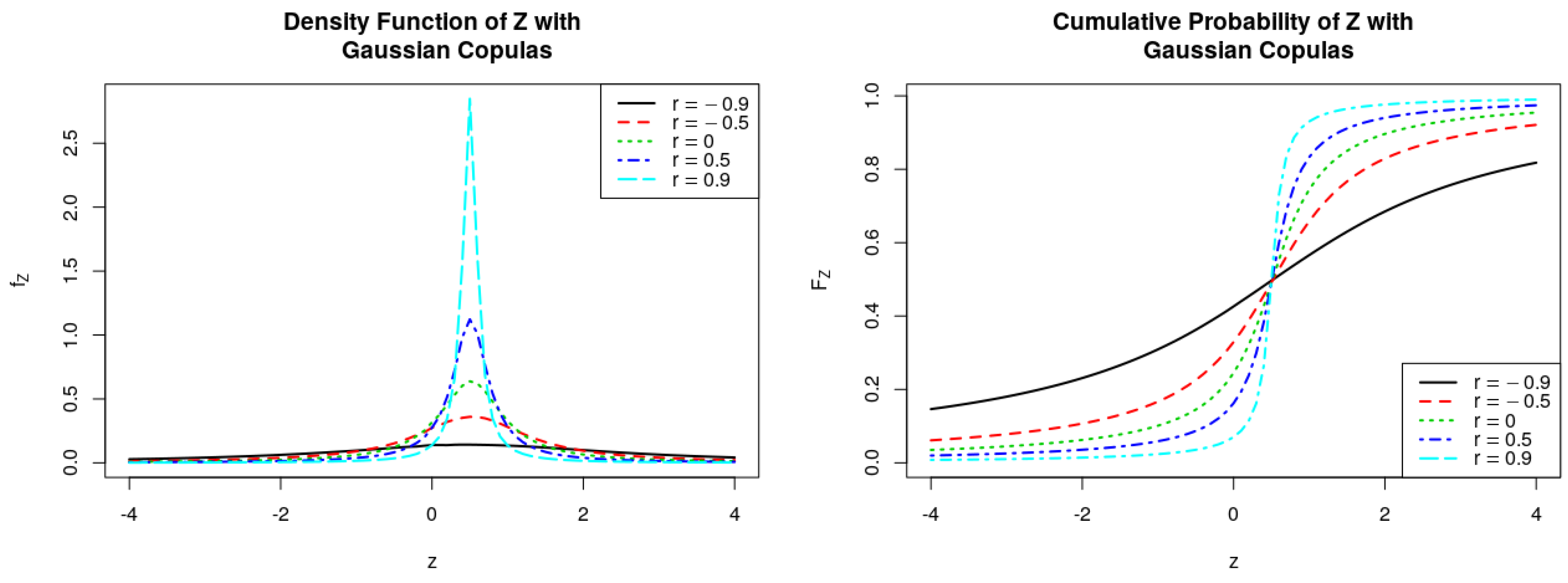
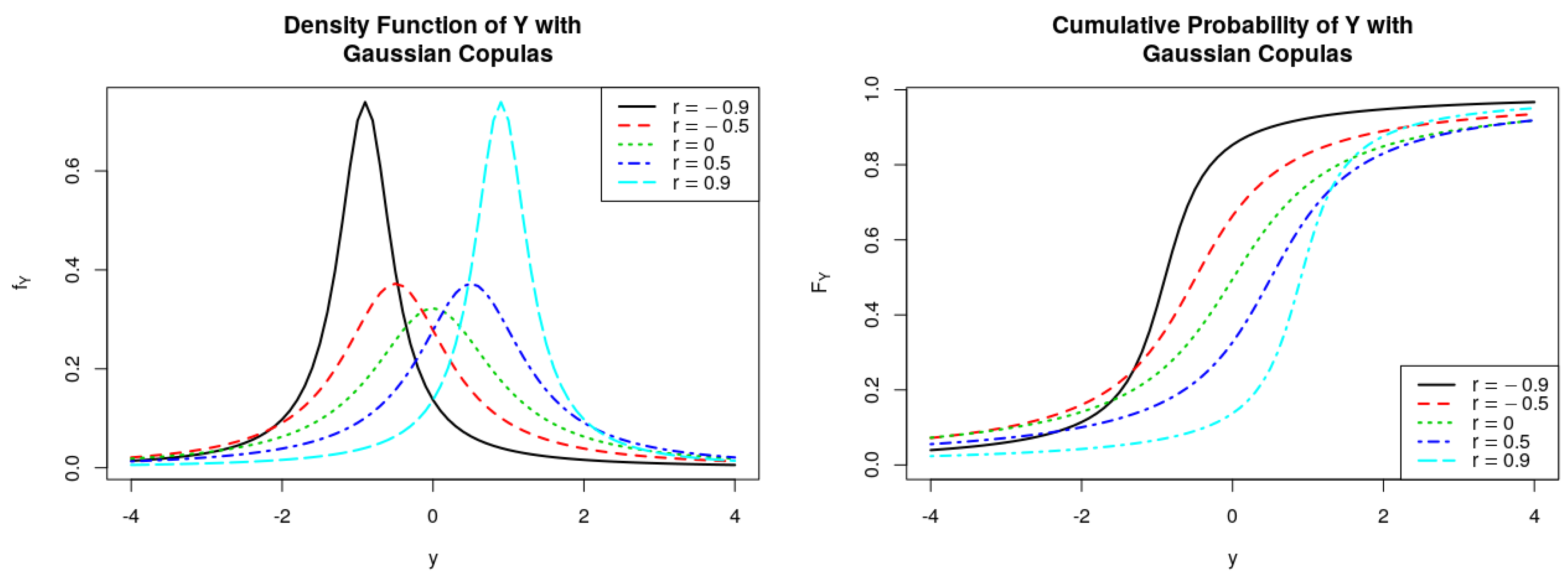
Figure 1.
PDFs and CDFs of the ratio , where follows Gaussian Copulas.
Figure 1.
PDFs and CDFs of the ratio , where follows Gaussian Copulas.
Figure 2.
PDFs and CDFs of the ratio , where follows Gaussian Copulas.
Figure 2.
PDFs and CDFs of the ratio , where follows Gaussian Copulas.
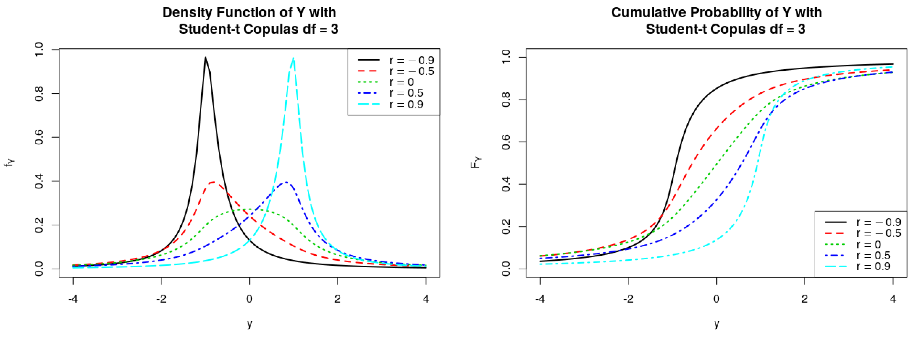
Figure 3.
PDFs and CDFs of the ratio , where follows Student-t Copulas, .
Figure 3.
PDFs and CDFs of the ratio , where follows Student-t Copulas, .
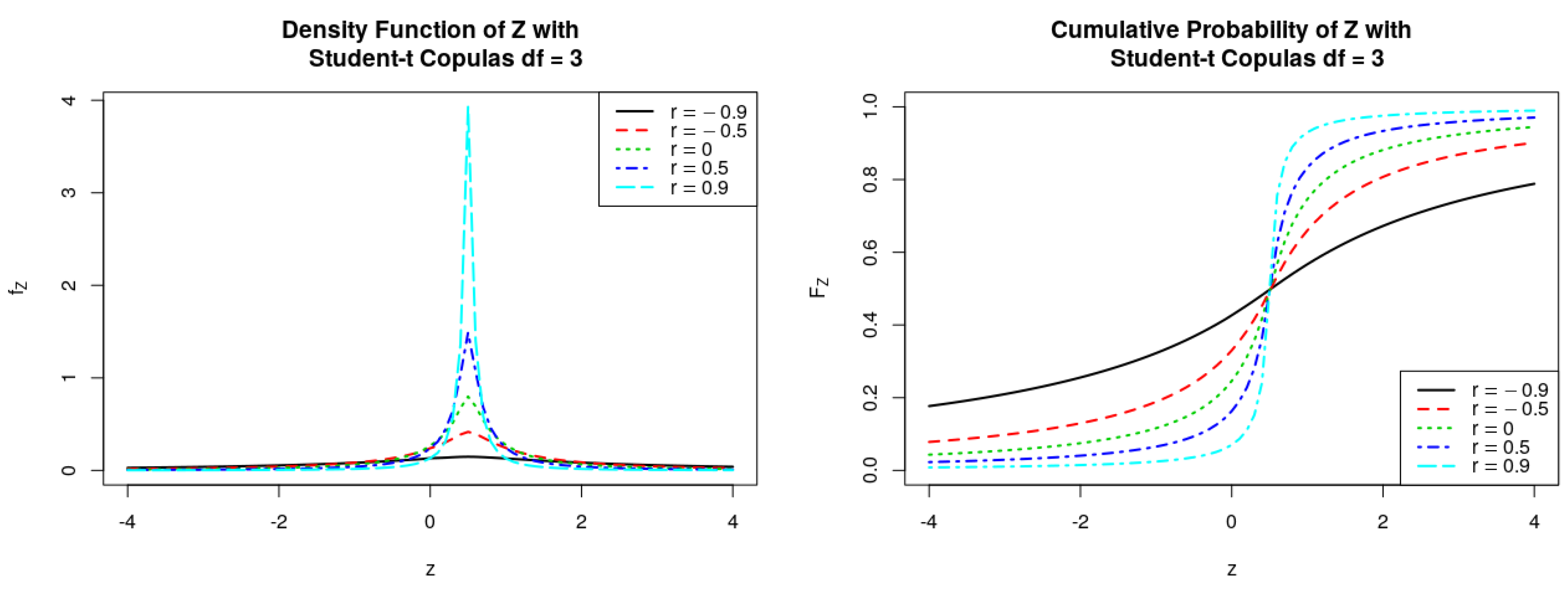
Figure 4.
PDFs and CDFs of the ratio , where follows Student-t Copulas, .
Figure 4.
PDFs and CDFs of the ratio , where follows Student-t Copulas, .
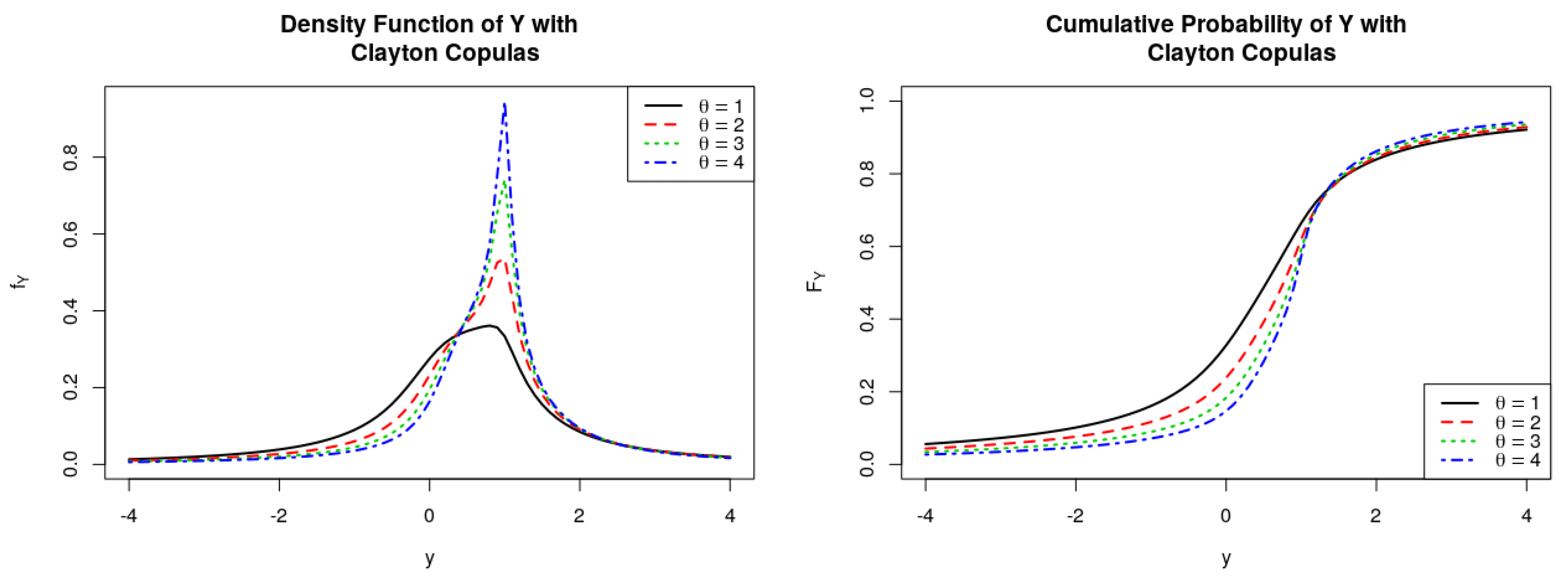
Figure 5.
PDFs and CDFs of the ratio , where follows Clayton Copulas.
Figure 5.
PDFs and CDFs of the ratio , where follows Clayton Copulas.
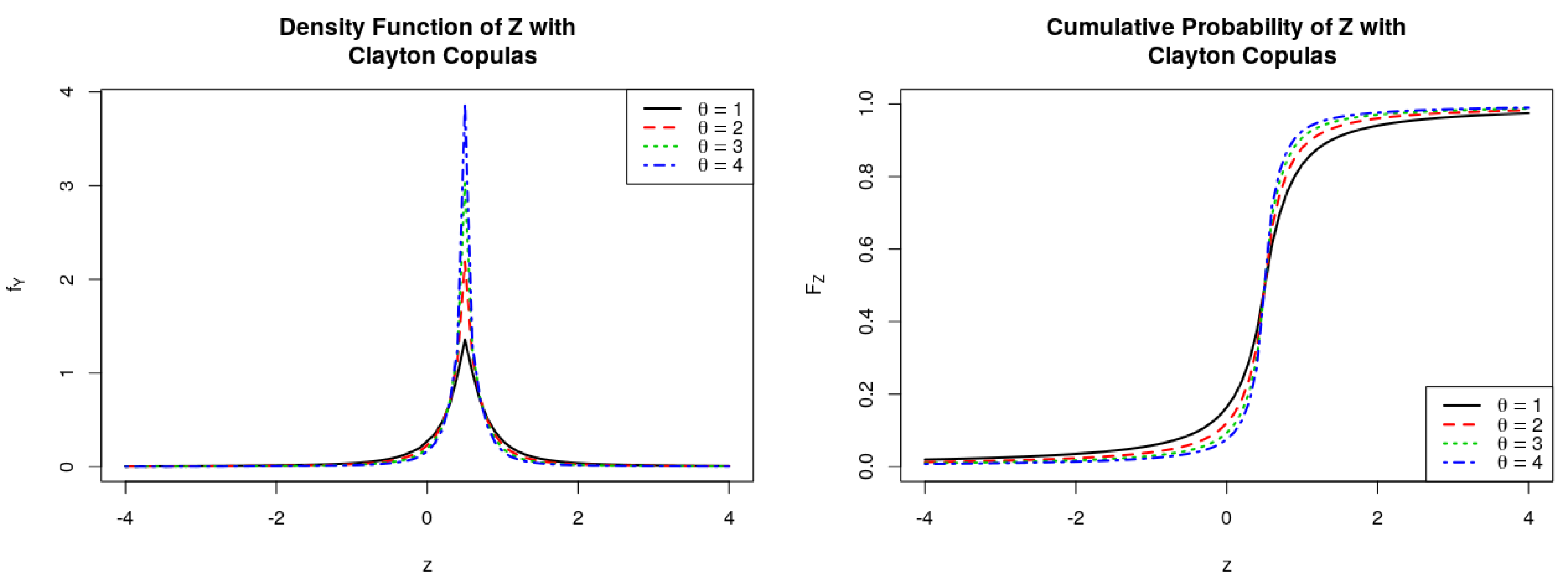
Figure 6.
PDFs and CDFs of the ratio , where follows Clayton Copulas.
Figure 6.
PDFs and CDFs of the ratio , where follows Clayton Copulas.
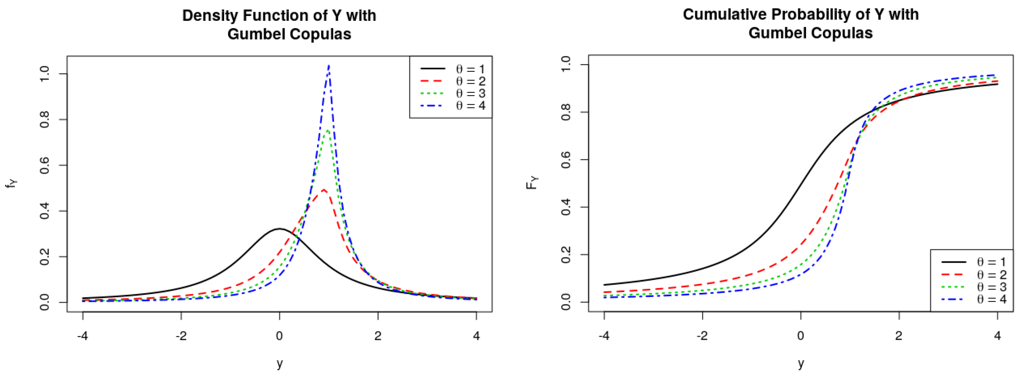
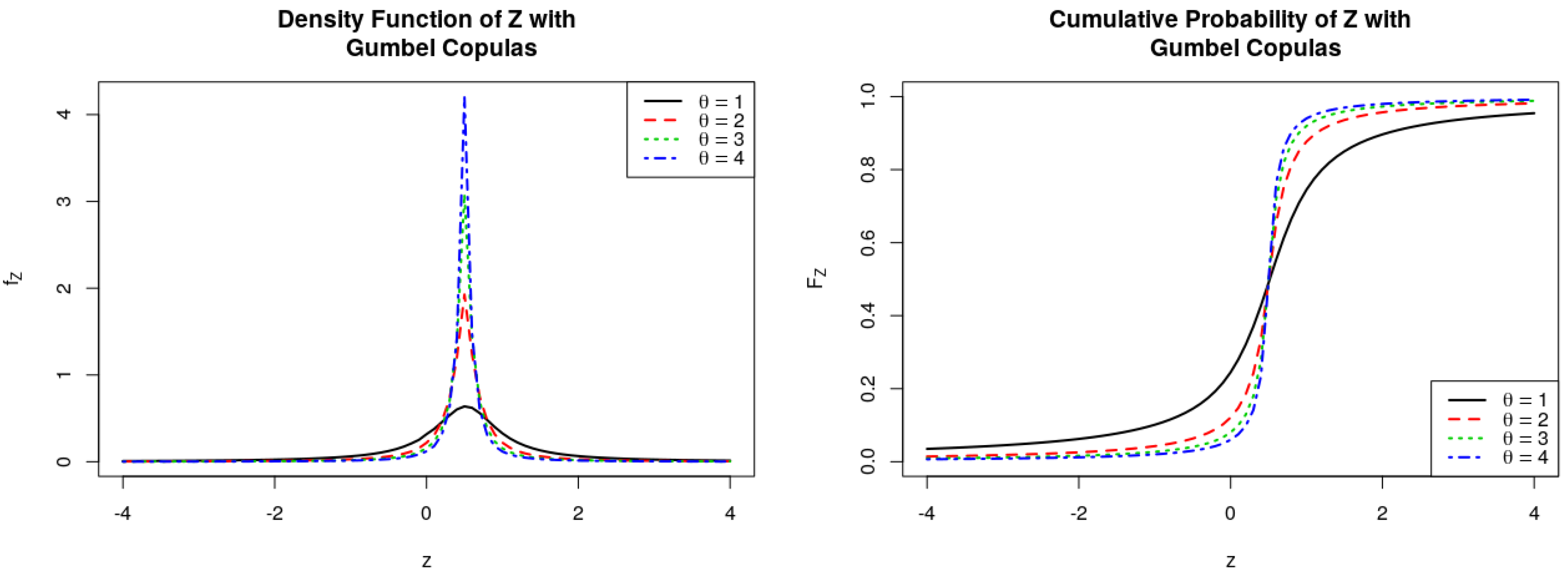
Figure 7.
PDFs and CDFs of the ratio , where follows Gumbel Copulas.
Figure 7.
PDFs and CDFs of the ratio , where follows Gumbel Copulas.
Figure 8.
PDFs and CDFs of the ratio , where follows Gumbel Copulas.
Figure 8.
PDFs and CDFs of the ratio , where follows Gumbel Copulas.
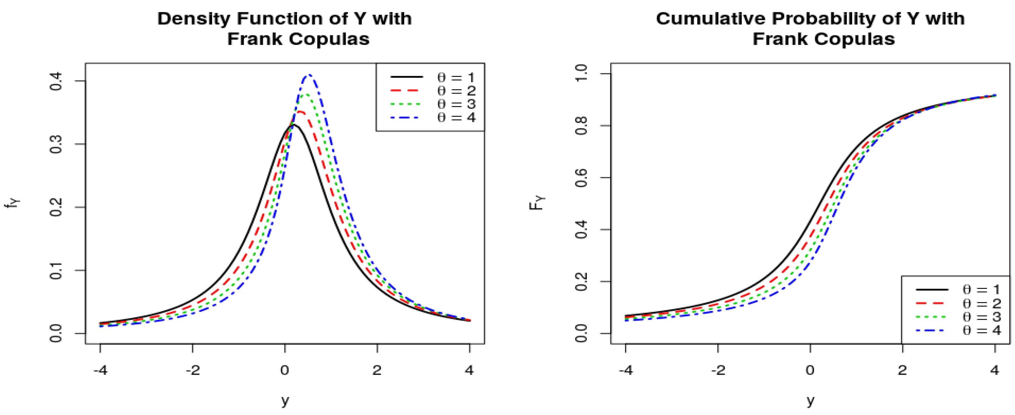
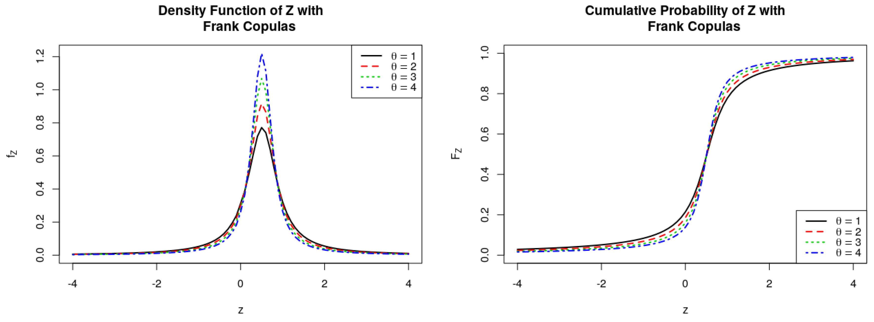
Figure 9.
PDF and CDF of quotient of the ratio , where follows Frank Copulas.
Figure 9.
PDF and CDF of quotient of the ratio , where follows Frank Copulas.
Figure 10.
PDF and CDF of the ratio , where follows Frank Copulas.
Figure 10.
PDF and CDF of the ratio , where follows Frank Copulas.
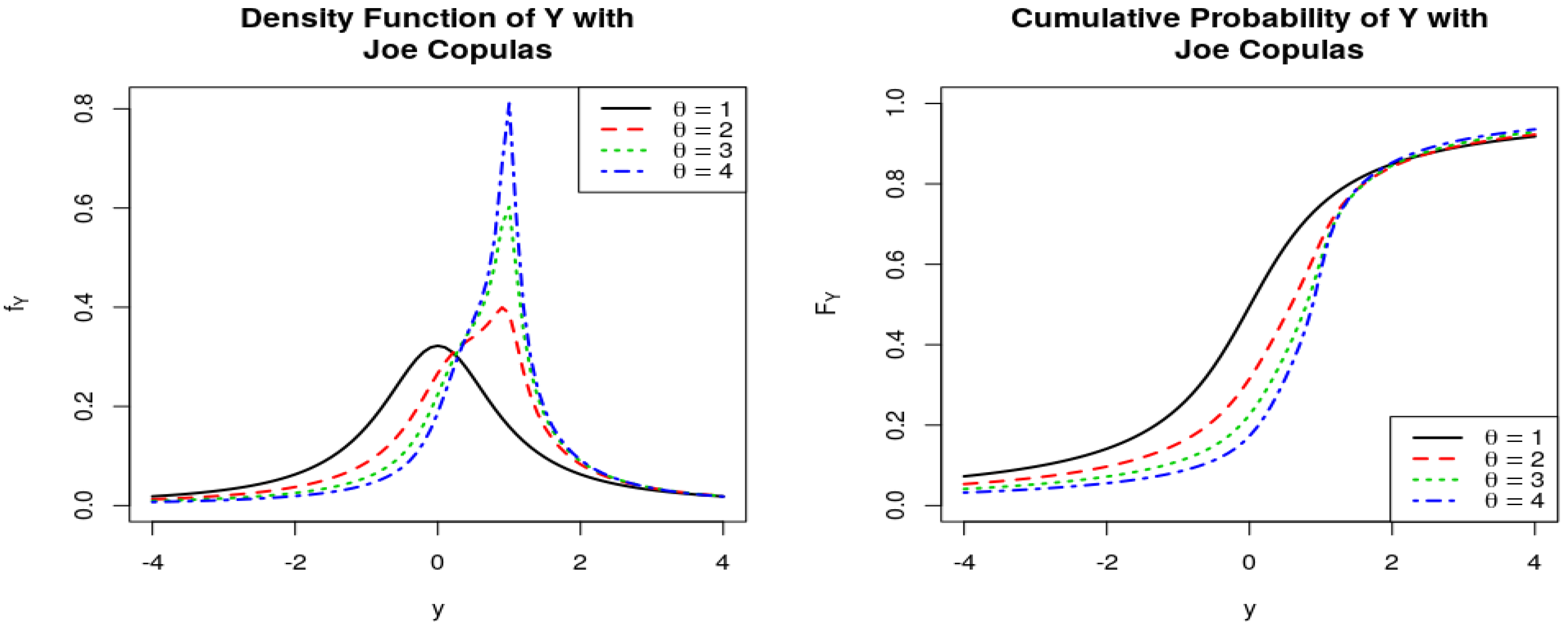
Figure 11.
PDFs and CDFs of the ratio , where follows Joe Copulas.
Figure 11.
PDFs and CDFs of the ratio , where follows Joe Copulas.
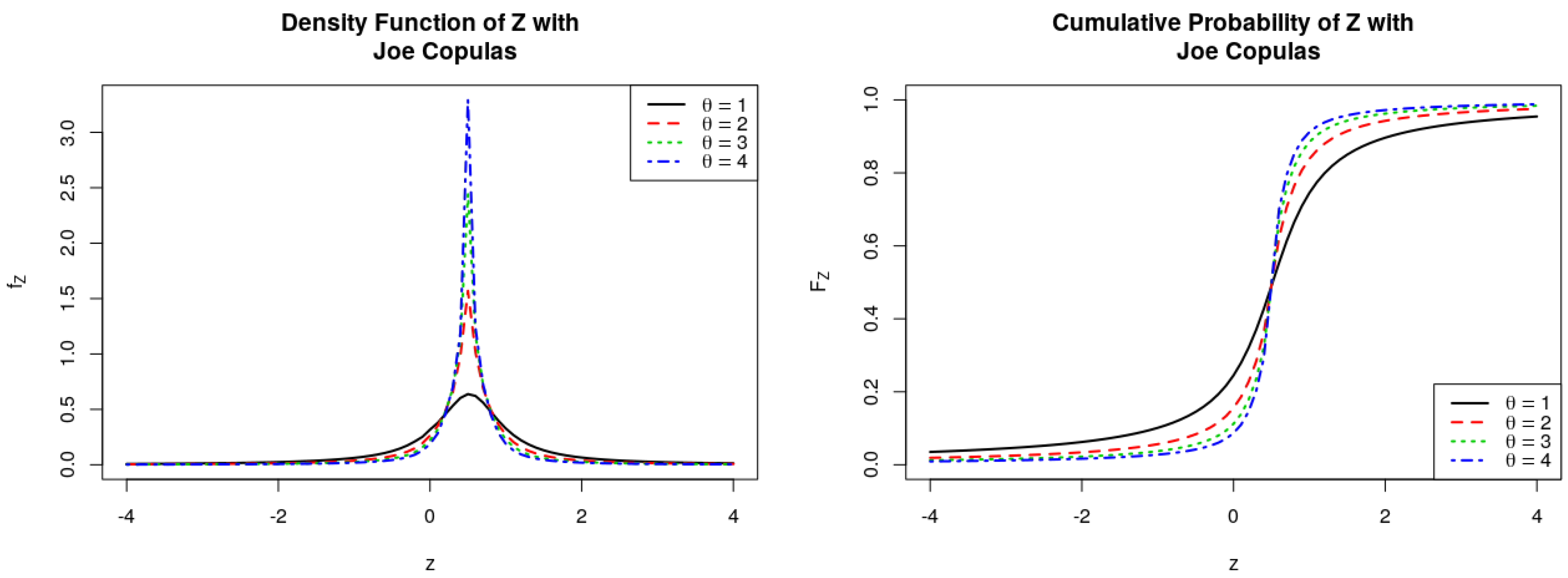
Figure 12.
PDFs and CDFs of the ratio , where follows Joe Copulas.
Figure 12.
PDFs and CDFs of the ratio , where follows Joe Copulas.
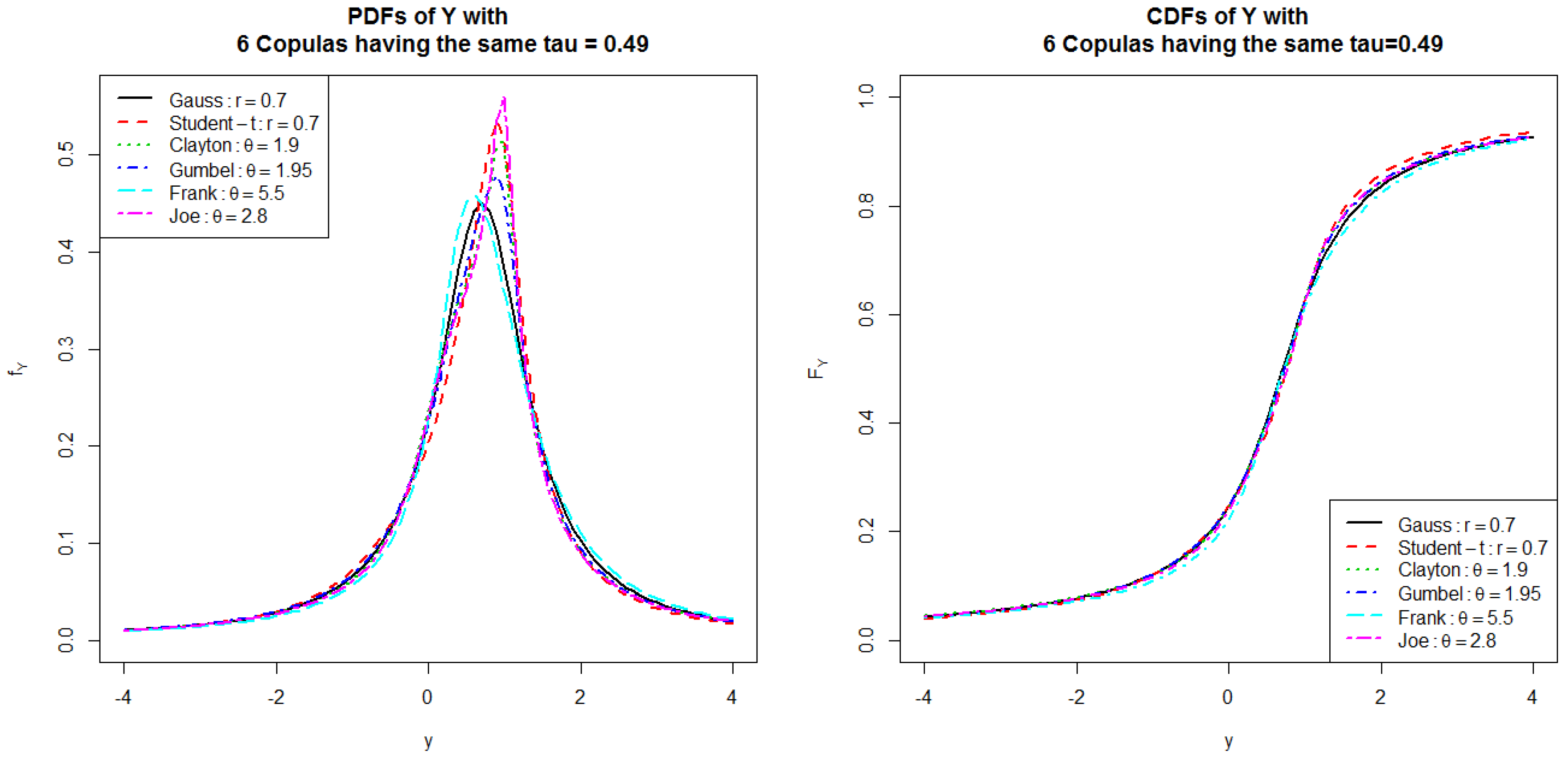
Figure 13.
PDFs and CDFs of the ratio , where modeled with six Copulas having the same .
Figure 13.
PDFs and CDFs of the ratio , where modeled with six Copulas having the same .
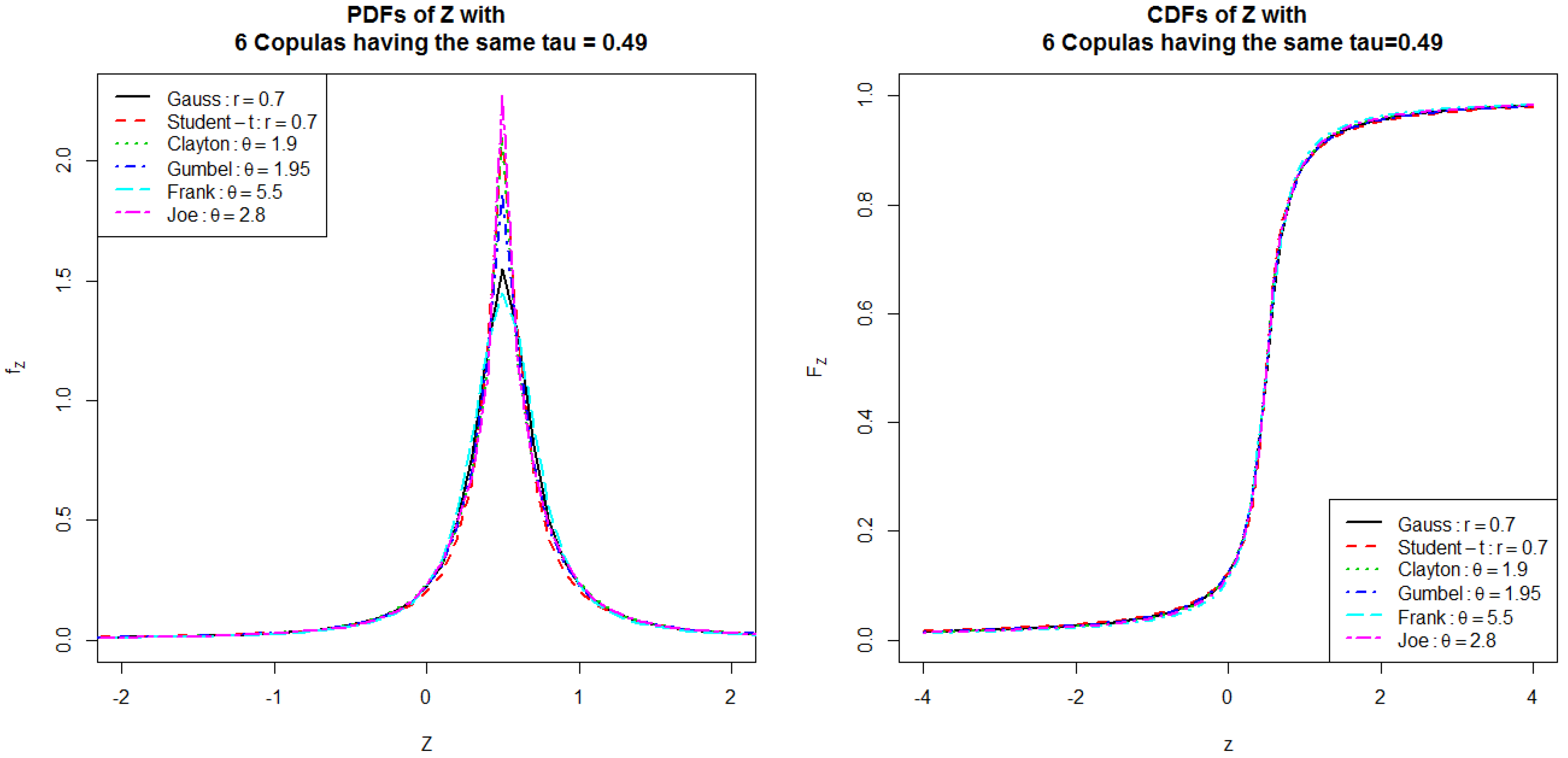
Figure 14.
PDF and CDF of the ratio , where modeled with six Copulas having the same .
Figure 14.
PDF and CDF of the ratio , where modeled with six Copulas having the same .
Table 1.
Some percentiles of , where follows Gaussian Copulas.
Table 1.
Some percentiles of , where follows Gaussian Copulas.
| r | | | | Median | | |
|---|
| | −3.65 | −1.34 | −0.9 | −0.46 | 1.85 |
| | −5.97 | −1.37 | −0.5 | 0.37 | 4.97 |
| 0 | 0 | −6.31 | −1.00 | 0.0 | 1.00 | 6.31 |
| 0.5 | 0.33 | −4.97 | −0.37 | 0.5 | 1.37 | 5.97 |
| 0.9 | 0.71 | −1.85 | 0.46 | 0.9 | 1.34 | 3.65 |
Table 2.
Some percentiles of , where follows Gaussian Copulas.
Table 2.
Some percentiles of , where follows Gaussian Copulas.
| r | | | | Median | | |
|---|
| | −13.27 | −1.68 | 0.5 | 2.68 | 14.26 |
| | −4.97 | −0.37 | 0.5 | 1.37 | 5.97 |
| 0 | 0 | −2.66 | 0.00 | 0.5 | 1.00 | 3.65 |
| 0.5 | 0.33 | −1.33 | 0.21 | 0.5 | 0.79 | 2.32 |
| 0.9 | 0.71 | −0.23 | 0.39 | 0.5 | 0.61 | 1.22 |
Table 3.
Some percentiles of , where follows Student-t Copulas, .
Table 3.
Some percentiles of , where follows Student-t Copulas, .
| r | | | | Median | | |
|---|
| | −3.42 | −1.26 | −0.92 | −0.50 | 1.82 |
| | −5.18 | −1.28 | −0.56 | 0.40 | 4.42 |
| 0 | 0 | −5.40 | −1.00 | 0.00 | 1.00 | 5.41 |
| 0.5 | 0.33 | −4.42 | −0.40 | 0.56 | 1.28 | 5.18 |
| 0.9 | 0.71 | −1.81 | 0.50 | 0.92 | 1.26 | 3.42 |
Table 4.
Some percentiles of , where follows Student-t Copulas, .
Table 4.
Some percentiles of , where follows Student-t Copulas, .
| r | | | | Median | | |
|---|
| | −18.20 | −2.05 | 0.5 | 3.05 | 19.21 |
| | −6.62 | −0.45 | 0.5 | 1.45 | 7.61 |
| 0 | 0 | −3.35 | 0.00 | 0.5 | 1.00 | 4.35 |
| 0.5 | 0.33 | −1.54 | 0.24 | 0.5 | 0.76 | 2.54 |
| 0.9 | 0.71 | −0.24 | 0.40 | 0.5 | 0.60 | 1.24 |
Table 5.
Some percentiles of , where follows Clayton Copulas.
Table 5.
Some percentiles of , where follows Clayton Copulas.
| | | | Median | | |
|---|
| 1 | 0.33 | −4.97 | −0.36 | 0.53 | 1.31 | 5.83 |
| 2 | 0.5 | −3.83 | 0.03 | 0.76 | 1.34 | 5.24 |
| 3 | 0.60 | −2.87 | 0.25 | 0.86 | 1.34 | 4.71 |
| 4 | 0.67 | −2.12 | 0.39 | 0.91 | 1.32 | 4.25 |
Table 6.
Some percentiles of , where follows Clayton Copulas.
Table 6.
Some percentiles of , where follows Clayton Copulas.
| | | | Median | | |
|---|
| 1 | 0.33 | −1.31 | 0.22 | 0.5 | 0.78 | 2.31 |
| 2 | 0.5 | −0.73 | 0.30 | 0.5 | 0.70 | 1.73 |
| 3 | 0.60 | −0.42 | 0.35 | 0.5 | 0.65 | 1.42 |
| 4 | 0.67 | −0.24 | 0.37 | 0.5 | 0.63 | 1.24 |
Table 7.
Some percentiles of , where follows Gumbel Copulas.
Table 7.
Some percentiles of , where follows Gumbel Copulas.
| | | | Median | | |
|---|
| 1 | 0 | −6.31 | −1.00 | 0.00 | 1.00 | 6.32 |
| 2 | 0.5 | −3.70 | 0.00 | 0.74 | 1.36 | 5.01 |
| 3 | 0.67 | −2.26 | 0.38 | 0.89 | 1.32 | 3.95 |
| 4 | 0.75 | −1.45 | 0.56 | 0.94 | 1.27 | 3.30 |
Table 8.
Some percentiles of , where follows Gumbel Copulas.
Table 8.
Some percentiles of , where follows Gumbel Copulas.
| | | | Median | | |
|---|
| 1 | 0 | −2.66 | 0.00 | 0.5 | 1.00 | 3.66 |
| 2 | 0.5 | −0.82 | 0.30 | 0.5 | 0.70 | 1.82 |
| 3 | 0.67 | −0.34 | 0.37 | 0.5 | 0.63 | 1.34 |
| 4 | 0.75 | −0.12 | 0.41 | 0.5 | 0.59 | 1.12 |
Table 9.
Some percentiles of , where follows Frank Copulas.
Table 9.
Some percentiles of , where follows Frank Copulas.
| | | | Median | | |
|---|
| 1 | 0.11 | −6.03 | −0.79 | 0.19 | 1.18 | 6.42 |
| 2 | 0.21 | −5.59 | −0.56 | 0.36 | 1.31 | 6.37 |
| 3 | 0.31 | −5.05 | −0.33 | 0.50 | 1.40 | 6.19 |
| 4 | 0.39 | −4.46 | −0.14 | 0.60 | 1.46 | 5.90 |
Table 10.
Some percentiles of , where follows Frank Copulas.
Table 10.
Some percentiles of , where follows Frank Copulas.
| | | | Median | | |
|---|
| 1 | 0.11 | −2.09 | 0.09 | 0.5 | 0.91 | 3.09 |
| 2 | 0.21 | −1.62 | 0.16 | 0.5 | 0.84 | 2.62 |
| 3 | 0.31 | −1.25 | 0.21 | 0.5 | 0.79 | 2.25 |
| 4 | 0.39 | −0.96 | 0.25 | 0.5 | 0.75 | 1.96 |
Table 11.
Some percentiles of , where follows Joe Copulas.
Table 11.
Some percentiles of , where follows Joe Copulas.
| | | | Median | | |
|---|
| 1 | 0 | −6.31 | −1.00 | 0.00 | 1.00 | 6.32 |
| 2 | 0.36 | −4.82 | −0.32 | 0.57 | 1.30 | 5.67 |
| 3 | 0.52 | −3.66 | 0.07 | 0.79 | 1.33 | 5.13 |
| 4 | 0.61 | −2.71 | 0.29 | 0.88 | 1.33 | 4.62 |
Table 12.
Some percentiles of , where follows Joe Copulas.
Table 12.
Some percentiles of , where follows Joe Copulas.
| | | | Median | | |
|---|
| 1 | 0 | −2.66 | 0.00 | 0.5 | 1.00 | 3.66 |
| 2 | 0.36 | −1.25 | 0.23 | 0.5 | 0.77 | 2.25 |
| 3 | 0.52 | −0.66 | 0.31 | 0.5 | 0.69 | 1.66 |
| 4 | 0.61 | −0.37 | 0.35 | 0.5 | 0.65 | 1.37 |
Table 13.
Some percentiles of , where modelled with six copulas having the same Kendall coefficient .
Table 13.
Some percentiles of , where modelled with six copulas having the same Kendall coefficient .
| Copulas | Parameters | | | | Median | | |
|---|
| Gaussian | 0.7 | 0.49 | −3.81 | −0.01 | 0.70 | 1.41 | 5.21 |
| Student-t | 0.7, | 0.49 | −3.52 | −0.02 | 0.76 | 1.31 | 4.63 |
| Clayton | 1.90 | 0.49 | −3.93 | 0.00 | 0.74 | 1.34 | 5.30 |
| Gumbel | 1.95 | 0.49 | −3.80 | −0.03 | 0.72 | 1.36 | 5.07 |
| Frank | 5.5 | 0.49 | −3.60 | 0.08 | 0.72 | 1.49 | 5.41 |
| Joe | 2.8 | 0.49 | −3.88 | 0.01 | 0.76 | 1.33 | 5.24 |
Table 14.
Some percentiles of , where modelled with six copulas having the same Kendall coefficient .
Table 14.
Some percentiles of , where modelled with six copulas having the same Kendall coefficient .
| Copulas | Parameters | | | | Median | | |
|---|
| Gaussian | 0.7 | 0.49 | | 0.29 | 0.5 | 0.71 | 1.83 |
| Student-t | 0.7, | 0.49 | | 0.31 | 0.5 | 0.69 | 1.92 |
| Clayton | 1.90 | 0.49 | | 0.30 | 0.5 | 0.70 | 1.77 |
| Gumbel | 1.95 | 0.49 | | 0.30 | 0.5 | 0.70 | 1.86 |
| Frank | 5.5 | 0.49 | | 0.29 | 0.5 | 0.71 | 1.65 |
| Joe | 2.8 | 0.49 | | 0.30 | 0.5 | 0.70 | 1.74 |


