1. Introduction
Let
be the prices of
N goods at discrete time instant
k. The evolution of the price can be modelled for
and
as
where
is the initial price of good
n and
is the relative price change of the
nth good between time
k and time
. Thus, if the price of good
n raises by
between time
k and time
, then
. The returns
are random variables whose knowledge is only limited at the level of some statistical properties. Thus, it is common practice to diversify the investor’s wealth among the
N goods, so that the entire capital is not reserved to a single good and that, in the case of a disastrous event (bankrupt), affect only the portion allocated to the unsuccessful good.
Markowitz’s Modern Portfolio Theory
Markowitz (
1952), sometimes referred as
Mean–Variance Approach, provides a method to choose an optimal allocation of wealth in view of knowledge of few statistical properties of the return variables. In particular, as the name suggests, this approach is based on the evaluations of the first- and second-order moments of
, and the investor can adopt the portfolio that maximizes the expected return given a maximum level of risk accepted. The relevance of this theory is enormous and it has been usually taken as a starting point in a variety of works in the context of portfolio optimization, as shown in
Elton and Gruber (
1997). Many of these works focus on overcoming some constraints of the original formulation of the Modern Portfolio theory. A point that has been deeply investigated in the past is how to deal with the estimation error that, due to the limited sample size, affects the mean and the variance (see
DeMiguel et al. (
2009),
Kritzman et al. (
2010)). In addition, the mean–variance approach has been compared to competitor approaches in the presence of unavoidable estimation errors (e.g.,
DeMiguel et al. (
2007),
Adler and Kritzman (
2007)). A criticism that has been moved to the mean–variance approach is about the possibility of describing the distribution of the returns in terms of two parameters only, the mean and the variance (basically, an assumption of Gaussianity). Papers that explore portfolio construction when distribution asymmetries and higher order moments are considered include those by
Cremers et al. (
2004),
Low (
2017), and
Low et al. (
2013,
2016).
Two assumptions impose severe limitations on modern portfolio theory. First, much of the literature assumes that mean and variance are knowable and known. Second, scholars often assume these two parameters alone describe the entire distribution. In addition, modern portfolio theory, as originally laid out, often presumptively forbids the use of short sales and leveraged positions. In other words, conventional works on portfolio design exclude borrowing, either for the purpose of profiting from declines in stock prices (short sales) or for the purpose of increasing the total volume of the investment and correspondingly the resulting profit or loss (leverage). Most studies concerned with these aspects (see
Jacobs and Levy (
2013a,
2013b) and
Pogue (
1970)) are based on complex methods and cannot be considered as simple extensions of the original theory.
In this paper, we move back to the original mean–variance approach assuming that mean and variance are known and present a simple extension of Markowitz’s theory, inspired by a well known principle in communication theory, that handles simultaneously short-sales and leverage. Finally, we also show that even transaction costs can be taken into account in a straightforward manner. The scope of the paper is thus two-fold: showing a connection between portfolio optimization and matched filter theory in communications, and providing a simple unified presentation of the mentioned important extensions to Markowitz’s original theory.
2. Trader Portfolio
We consider here the financial activity commonly called trading. The distinction that we make between investing and trading, and that we exploit in the present paper, is that in the latter short trading and leveraged trading are allowed. Basically, this means that in trading money is used not merely to buy assets, but to guarantee risky positions that can remain open until the occurrence of a stop loss condition. When the stop loss condition occurs, the position is closed and money used to guarantee it is lost.
The time evolution of a
leveraged position on good
n is
where
is the money invested on good
n at time
k,
is the leverage factor (we return on the meaning of
later on), and
is the long/short indicator. Hence,
when the position on good
n at time
k is long, while
when the position is short. In the following, we assume that
meaning that position on good
n has been closed at time
because all money used to guarantee it has been lost. Basically, Equation (
2) describes the evolution of a financial product that invests with directionality indicated by
and leverage
on good
n, and that consolidates its value at each iteration.
The portfolio is the sum of leveraged positions, that is
The evolution of the portfolio for
, is
The iteration terminates at time instant
K such that
The relative return of the positions taken at time
k, which is the focus of the following analysis, is
In the following, we consider one step of the iteration and withdraw the time index, thus writing
It is convenient to write the relative return of the portfolio as
where
is the relative return of position
n with
and
Note that
hence
is the relative money invested on good
n and
is a leverage factor that can be set equal for all goods without affecting the relative return of the portfolio. Although the leverage factor of stocks is often an integer, the trader may obtain any real value of the leverage by mixing positions on the same good with different leverages. Note that leverages between 0 and 1 can also be obtained simply by investing with leverage 1 a fraction
of the available money while letting a fraction
be cash. In the end, the real limit on
is determined by the maximum leverage available on the financial market, which is in practice so high that we can ignore the limits that it poses.
3. Portfolio Optimization
Let boldface lowercase characters denote column vectors and boldface uppercase characters denote matrices, and let
where the superscript
denotes transposition, be a multivariate random process representing the market behavior with mean vector
and covariance matrix
where
denotes expectation. In the following, we assume that the above mean vector and covariance matrix are known.
For any
, portfolio optimization requires of finding the relative money allocation vector
that maximizes the mean value of the relative return (Equation (
9)) with a fixed variance of the relative return. Note that the optimal portfolio will include only positions with
that is with
because positions with negative expected return will be outperformed by cash. For this reason, without losing generality, we consider in the following only
being understood that, when
, one takes
and then puts
With these assumptions, for any
, portfolio optimization requires of determining the vector
that maximizes the expected relative return with a fixed variance of the relative return and with the constraints in Equations (
13) and (
14). This is a classical constrained optimization problem that can be worked out by maximizing the Lagrangian
where
is the Lagrange multiplier and the constraints are Equations (
13) and (
14). Writing the relative return as
one promptly finds that the mean value and the variance of the relative return are
and
respectively. Hence, the Lagrangian is
Assuming that
is definite positive, hence invertible, it is easy to see that the unique maximum of Equation (
26) is achieved with
where
Imposing Equation (
14), one finds
which, substituted in Equation (
27), leads to
Note that, since
is definite positive, its inverse is also definite positive and, since all the entries of
are non-negative, all the entries of
are non-negative, and hence the constraint in Equation (
13) is always satisfied. Equations (
28) and (
30) say that the relative weights of positions in the optimal portfolio are fixed and independent of the risk that the trader wants to take, while the balance between expected return and risk can be tuned by tuning the leverage according to Equations (
24) and (
25).
The performance of the optimal portfolio is characterized by the following expected relative return and variance of the relative return
The
unconstrained efficient frontier is a straight line in the first quadrant of the plane
that departs from
and that has slope
that is the Sharpe ratio (see
Sharpe (
1966)), a figure that has been object of many studies after the original paper by Sharpe (see, e.g.,
Bailey and Lopez de Prado (
2012) for estimates of the Sharpe ratio when
and
cannot be assumed to be known). The entire efficient frontier can be visited by sweeping
from 0 (zero expected return) to
∞ (infinite expected return). Note that including explicitly a risk free position in the portfolio would lead to a covariance matrix that is not invertible, while, with our approach, the risk free position is automatically brought into the portfolio when
, because a fraction
of the portfolio is cash.
1As shown in
North (
1963) and
Turin (
1960), Equations (
28) and (
33) are very well known in the context of narrowband discrete-time Single Input Multiple Output (SIMO) transmission systems affected by correlated additive noise, e.g. interference. In that context, the transmission channel is characterized by applying an impulse to the input and by collecting the
N channel outputs into vector
. In addition, channel’s output is affected by zero-mean additive noise with covariance matrix
. Vector
is the
matched filter (MF), that is the vector of weights that, applied to the multiple outputs, that is to the goods held in the portfolio, produces through Equation (
9) the least noisy version of the input impulse in the mean-square error sense, while
is the
Signal-to-Noise Ratio (SNR) after the matched filter. The application of the matched filter in portfolio optimization is not new, as illustrated by
Pillai (
2009), where however it is shown only how the said communication theory technique can be exploited in investing contexts, without any extension to trading. To put more light on the link between communication theory and the subject treated in this paper, we point out that, in the context of communication theory, the random vector
introduced in Equation (
15) can be regarded as the vector signal at the output of a SIMO channel excited by an input impulse of unit amplitude:
where
is a vector that, in the communication context, is the impulse response of the SIMO channel, and
is a random noise vector having zero mean values and covariance matrix
(also the covariance matrix of the noise vector is assumed here to be known). As pointed out by an anonymous referee, the suggestion of regarding the variability in financial returns as the effect of noise (the Brownian motion of gas) dates back to Bachelier’s thesis
Bachelier (
1900). At the receiver side, the received vector is passed through the matched filter (Equation (
30)), getting
where, in the context of communication, the scaling factor
is set to
so that
meaning that
r recovers the unit amplitude of the input impulse keeping minimum the mean squared error
, hence achieving the maximum of Equation (
33). Besides this, the matched filter has another interesting property that is well known in the context of communication and information theory. Let
a be a random scalar parameter that, in the context of communication, is the information-carrying amplitude, e.g.,
. When an impulse of amplitude
a is applied at channel input, the channel output is
With Gaussian noise, the matched filter output
is a
sufficient statistic for the hidden
a. This means that
r can be seen as a synthetic representation of
that fully preserves the possibility of making inference, for instance, maximum likelihood detection, about the hidden
a based on
r alone. In a more technical language, this concept is expressed by saying that the information processing inequality
where
is Shannon information between
x and
y, is met with equality when the transformation
is the right hand side of Equation (
38). The interested reader is referred to Chapter 2 of
Cover and Thomas (
2006) for the basics about Shannon information, for the concept of sufficient statistic and for the meaning of the information processing inequality.
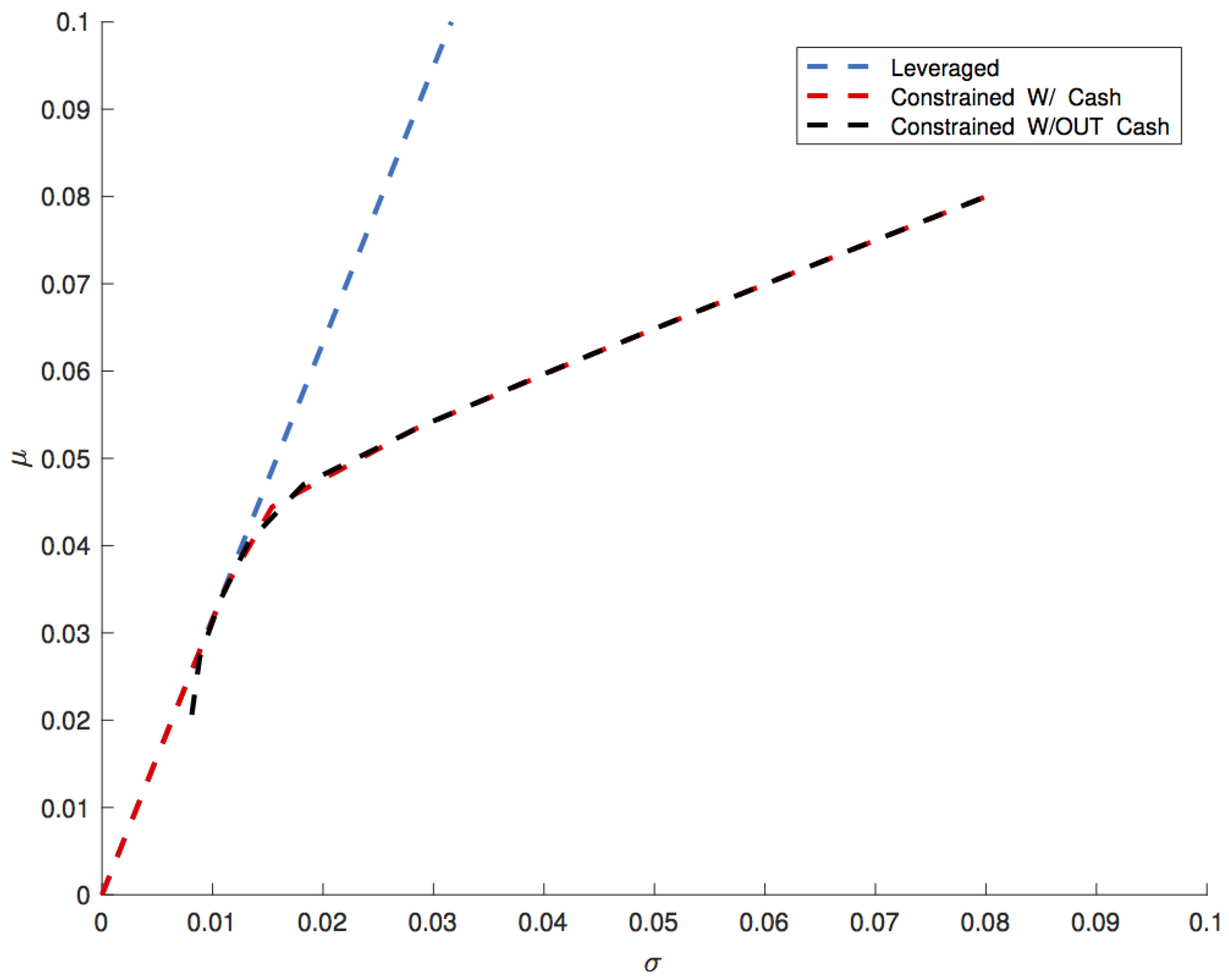
An example illustrates similarities and differences between the leveraged portfolio and classical Markowitz’s portfolios. Consider three goods with
For the leveraged portfolio, the optimal money allocation vector is proportional to
and the slope of the efficient frontier is
Figure 1 reports
versus
for the individual goods and the efficient frontiers for the leveraged portfolio and for the Markowitz’s portfolios with and without the possibility of holding cash.
What happens is that the efficient frontier of the Markowitz’s portfolio without cash is equal to the efficient frontier of the leveraged portfolio until
because the fraction
of cash of the leveraged portfolio is invested in the non-leveraged portfolio on the low risk stocks, thus leaving the performance of Markowitz’s portfolio only slightly worse than the performance of the leveraged portfolio. In the limit, including the possibility of holding cash in Markowitz’s portfolio would close the gap between leveraged and non-leveraged portfolios until the inequality in Equation (
43) is satisfied. Differences between the two portfolios become bigger and bigger as
because, while the leveraged portfolio continues taking profit from diversification by maintaining the optimal mix between goods thanks to the big leverage, the absence of leverage forces the Markowitz’s portfolios to renounce to diversification, leading in the limit to a portfolio composed by only one good, the one that offers the greater expected return, even if, as it happens in the example, this portfolio could be easily outperformed also by a portfolio made by only one good with better
, simply by leveraging it.
4. Cost of Transactions
Another relevant feature not considered in Markowitz’s original paper is the cost deriving from a transaction on the market.
Transaction costs may influence portfolio’s optimization, and, for this reason, transaction costs have been widely considered in the subsequent literature (
Lobo et al. (
2007),
Mansini et al. (
2003),
Mansini and Speranza (
1999,
2005)). Type and structure of transaction costs depend on the financial operator (e.g., broker or bank) and on the type of stocks that the trader uses for her/his operation (e.g., Exchange Trade Commodities, Exchange Traded Funds, or Contract for Difference). Let us consider a general case where the relative cost is of the type
where, here again, without losing generality, we assume that the leverage factor is common to all the goods and consider a transaction cost that can depend on the specific good and on the leverage factor. The relative return of the
nth position is
By following the steps of Equations (
19)–(
21), we consider only the case in Equation (
20), with the more demanding condition
The above inequality means that a position that does not meet the above inequality cannot be in the portfolio, because it is outperformed by cash. A brief comment about the dependence of
on
is in order. Consider the investment in bonds with one-year life emitted by a very trusted central bank. If the time step is one year and the return of the bond is higher than the cost of transaction, then one could borrow money to buy bonds. Actually, this is allowed in our model, because borrowing money simply means increasing
. However, in a case like the one of this example, borrowing money is a cost that increases the cost of transaction, so that, in the end, the cost of transaction becomes higher than the return of the bond. When this happens it is the dependence of
on
that, through Equation (
46), rules out this position from the leveraged portfolio. Actually, a realistic cost model for such a case is
where
takes into account costs such as bank commissions that apply when investor’s money is employed, that is for
, while
takes into account the cost of borrowing money, which applies to a fraction
of the investment. If, for
,
then the condition in Equation (
46) is violated and the position on good
n with leverage
cannot be included in the portfolio.
The constrained optimization is again Equation (
22) with the usual constraints, but now
The optimal portfolio and the efficient frontier are found by the same means as in the previous section, simply putting in place of The only difference is that, when the cost of transactions depends on , the optimal portfolio will depend on and the efficient frontier will no longer be a straight line.
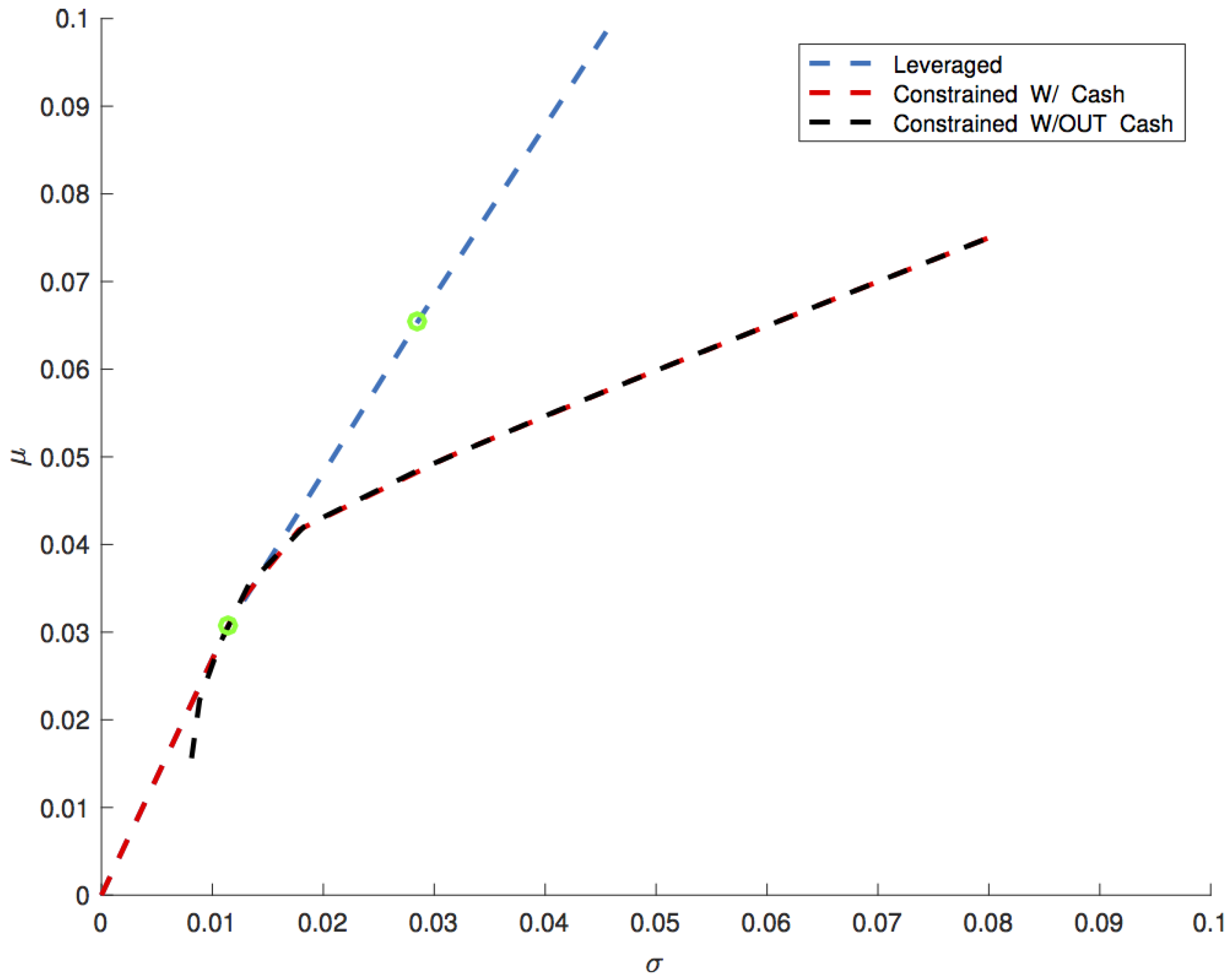
As an example, we consider again the example of
Section 3 where the statistical properties are described by Equations (
41) and (
42) with the addition of the following transaction costs
equal for the three goods.
Figure 2 displays a new comparison between Markowitz’s portfolios and leveraged portfolio with the inclusion of transaction costs (Equation (
50)). The first region corresponds to
, where the efficient frontier of the leveraged portfolio is a straight line since we are in the first case of Equation (
50), where
is actually a constant since there is no dependance of
. The breakpoint between the straight line and the second region is at
, where the transaction cost changes and is no longer independent of
as in the second case of Equation (
50). The separation between the second and the third region is at
, where
and good 1 is ruled out by Equation (
46). Finally, as
, the efficient frontier approaches a straight line, because
approaches the constant
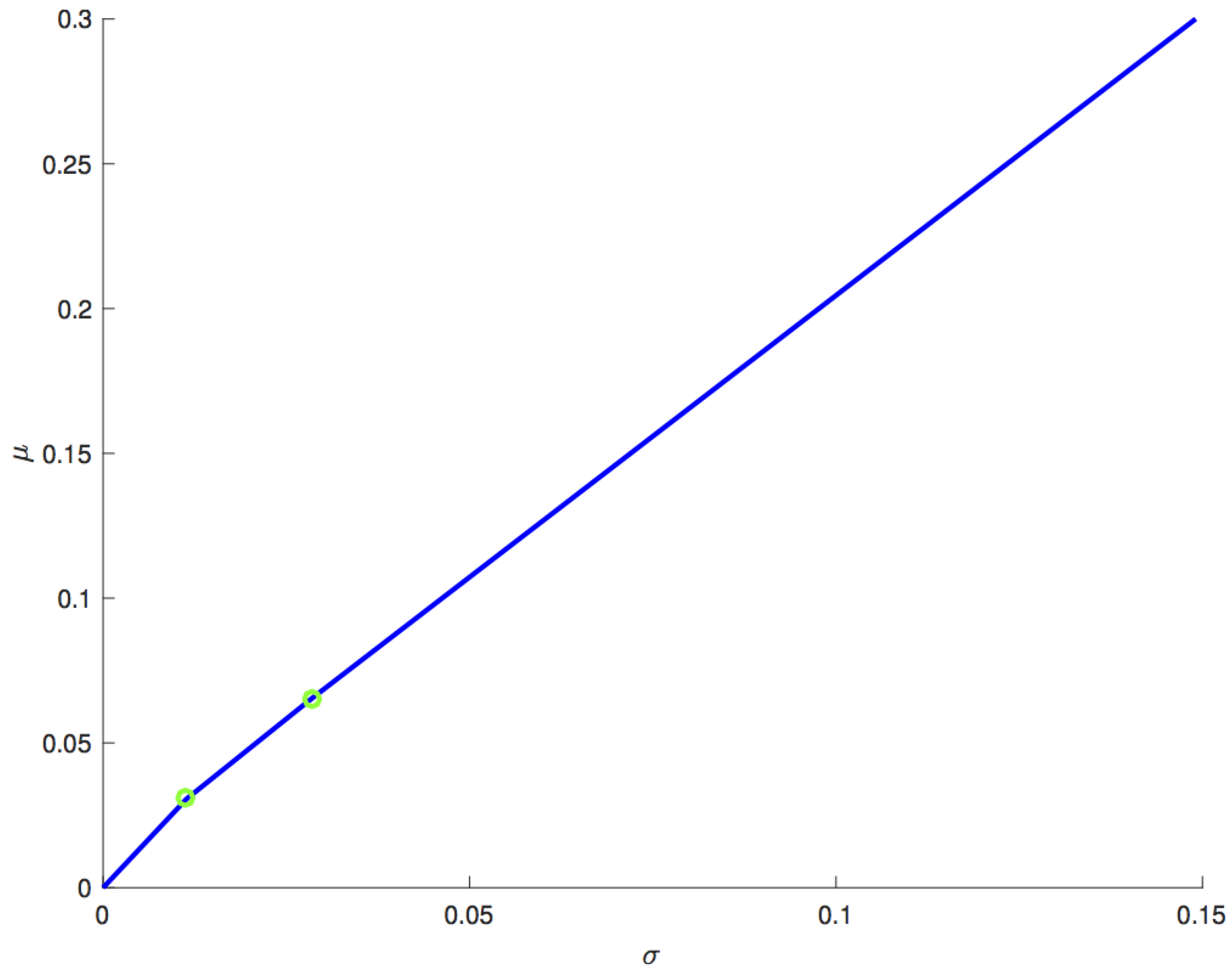
. These features are not easily noticed in
Figure 2. Thus, in
Figure 3, the efficient frontier of the leveraged portfolio is illustrated from a different perspective, where the division in three different regions highlighted by green dots is more visible.


