Article

Take Profit and Stop Loss Trading Strategies Comparison in Combination with an MACD Trading System

by
Dimitrios Vezeris
1,*,
Themistoklis Kyrgos
2 and
Christos Schinas
1
1
Department of Electrical and Computer Engineering, Democritus University of Thrace, 67100 Xanthi, Greece
2
COSMOS4U, 67100 Xanthi, Greece
*
Author to whom correspondence should be addressed.
J. Risk Financial Manag. 2018, 11(3), 56; https://doi.org/10.3390/jrfm11030056
Submission received: 22 August 2018 / Revised: 14 September 2018 / Accepted: 17 September 2018 / Published: 19 September 2018
(This article belongs to the Special Issue Empirical Finance)

Abstract

:
A lot of strategies for Take Profit and Stop Loss functionalities have been propounded and scrutinized over the years. In this paper, we examine various strategies added to a simple MACD automated trading system and used on selected assets from Forex, Metals, Energy, and Cryptocurrencies categories and afterwards, we compare and contrast their results. We conclude that Take Profit strategies based on faster take profit signals on MACD are not better than a simple MACD strategy and of the different Stop Loss strategies based on ATR, the sliding and variable ATR window has the best results for a period of 12 and a multiplier of 6. For the first time, to the best of our knowledge, we implement a combination of an adaptive MACD Expert Advisor that uses back-tested optimized parameters per asset with price levels defined by the ATR indicator, used to set limits for Stop Loss.

Graphical Abstract

1. Introduction

When trading on an asset, investors are exposed to a potentially high risk if the price moves towards a direction which is the opposite from the one they had anticipated. This could result in considerable losses in the investment capital, unless immediate action is taken to exit the non-profitable position as soon as possible. On the other hand, if the price moves towards a direction that makes the current position profitable, an investor might want to close the position and cash in the profits gained so far, as there is always the possibility that winning trades could turn into losing positions and lead to catastrophic losses.
Different strategies of securing profits (Take Profit) and averting losses (Stop Loss) have been proposed and examined, usually involving the prices at which a position was opened, and are frequently used by traders, as well as automated trading systems. In this research, we tested and compared six different Take Profit and Stop Loss strategies used in combination with an algorithmic trading system, based on the MACD indicator on eleven different assets over a six-month period. With the results of these comparisons, we aim to provide some practical insights into every day traders about which Take Profit and Stop Loss technics to incorporate with an existing MACD strategy and which to avoid. There have been numerous studies about MACD, which is a 30-year-old tool, such as those by Chong and Ng (2008) and Yazdi and Lashkari (2013), focused on MACD’s performance in various markets and timeframes, or such as that by Ni and Yin (2009), who examined, among others, Take Profit and Stop Loss technics in MACD using neural networks. But there has not yet been a study of MACD combined with the Take Profit/Stop Loss strategies we examined based on ATR and in a faster timeframe.

2. Materials and Methods

2.1. Trading Systems

2.1.1. Automated Trading

Nowadays, trading is almost exclusively conducted electronically through a computer (Jain 2005). In addition to that, investors have replaced the broker with a platform of automated trading (algorithmic trading), as was postulated by Hendershott and Moulton (2007).
The decrease in the cost of this technology has led to its fast-paced adoption by the financial industry. The resulting technological change has brought about a revolution in the financial markets and the way the assets are traded. Many institutions today trade through algorithms and algorithmic trades improve liquidity. It has been proven that the increased algorithmic trades limit wrong price choices and decrease the proportion of offer risk over different price levels of an asset associated with the trades. These results show that algorithmic trading lowers the cost of trades and enhances the informativeness of quotes, as demonstrated by Hendershott et al. (2011).
On the other hand, it seems that Forex manual trading outweighs automated trading systems. Humans are more informed than systems (Chaboud et al. 2014). However, on closer inspection, we realize that there are some indications pointing to the fact that algorithmic trading contributes to an efficient price discovering process (Brogaard et al. 2014) through the elimination of opportunities for triangular arbitrage and faster “integration” of macroeconomic news into the price (Foucault et al. 2011). Also, in the same paper, it was established that algorithmic trades tend to correlate, demonstrating that automated strategies are not that different from those used by a human. Despite that correlation, there are no indications that algorithmic trading causes excess variability. In addition, the volume of algorithmic trading in the market has a small, but positive, impact on the liquidity of the market.
In this research, only algorithmic trades are executed without human intervention, with an automated high frequency trading system. Consequently, commissions and the cost of position swap are kept to a minimum, in contrast with using human intermediaries, and are subsequently presented. But the main element is the fact that they are automatically included in the results by the trading terminal we used. Consequently, the profit rate presented in this paper is pure, after the deduction of commissions.

2.1.2. Private Investors

As more brokers adopt electronic trading platforms, more private investors opt for automated algorithmic trading. It is estimated that private investors lose 2% in the USA market and 3.8% in Taiwan annually (Barber et al. 2008). It has also been calculated that institutional profits are enhanced by 1.5% annually as a result of the small transactions’ cost and corresponding profits of the same actions.
The feeling of the individual investors in relation to weekly and monthly profits and the variability of NYSE stocks was studied by Kaniel et al. (2004). Private investors who are more aware of the risk may force them to provide liquidity to other market participants who seek an instant service. The buying orders from bigger, stock-accumulating investors can cause a coercion of sales by increasing the prices. In the same way, individual buyers are attracted to lower prices caused when these larger investors choose to sell their stocks. Liquidity is actually provided by both professional traders (e.g., specialists) and individuals. If we assume that market liquidity is only provided by individual investors and they are more active in relation to the demand for immediacy, then there would be an excess supply of liquidity. In this case, individual investors that have contracts and are silent liquidity providers will amount losses, while more terms-informed investors will perform trades in adverse conditions. If, on the other hand, there are fewer investors than the market immediacy demands, the silent liquidity providers will amount profits. Understanding the predictability of the short-term profits calls for an understanding of the silent liquidity provision to individuals, as well as the explicit liquidity provision to professional investors. Specifically, the provision of liquidity can be regarded as the interaction between different types of investors that trade on the same market.
A lot of individuals, in parallel with these systems, adopt long-term positions, instead of strategic buying and holding, strategies whose trends are reflected on Google Trends, an analysis by Preis et al. (2013) quantifying the behavior of the market. In this research, there is no liquidity problem, especially for the $10,000 of initial capital, as the automated systems tested in this research can be implemented by institutes, as well as by private investors. On the other hand, it has been proven through back-testing that whether or not data from the profits of an asset or data from Google Trends are used for the same asset, the results are the same. The results have been tested on a non-linear machine learning system by Challet and Ayed (2014). In the current work, the problem of back-testing period selection is evident.

2.2. Take Profit & Stop Loss

Returns can be either absolute or relative. As a rule, we avoid absolute numbers because they will have to be calculated for each asset individually. Leung and Li (2015) proved that the stop loss function has to be calculated at every moment because it is related to the price of an asset at every tick since that price is within the price range x ∈ (L, b × L), or the investor, if x is the entering price, can simply set a constant I (proportional to the fluctuation we add), where x−I is the stop loss price. In addition, returns change over seasons and periods, according to the influences an asset undergoes as a result of outside or inside factors. It is obvious that orders with stop loss and take profit, when activated, oppose the market trend (take profit) or intensify the movement (stop loss), with great influence even over the liquidity during a flash crash (Easley et al. 2011). In all these adoptive trading systems, special consideration should be given to the use of these functions, as shown by Austin et al. (2004). In addition, the use of cut-loss orders and take profit orders and the range of these orders reflect the risk-taking desire of the investor (Au et al. 2003).
With regard to absolute numbers, we see a 3% take profit and a 2% stop loss in the work by Bolgün et al. (2010) on stocks of the Istanbul Stock Exchange. Constant take profit was used by Krishnan and Menon (2009), defined at 20 pips, in an interesting work that examined the influence that rate, closing price times, and indicators participating in trading systems (RSI, BB, Stoch, SAR, MACD, ADX, CCI, Williams %R, Mom, A/D) have on profit. Take profit was also set at 20 pips by Barbosa and Belo (2010). Even in systems that are based on the flow of buy and sell orders and not on the price itself, as postulated by Bates et al. (2003), stop loss and take profit were used as a function of returns 0–0.5%, 0.5–1%, etc. Similarly, Azzini and Tettamanzi (2008b) set staggering take profit signals on returns of 0.33%, 0.67%, etc., while in another work, Azzini and Tettamanzi (2008a) took three returns as take profit, logarithmically setting the constant at rTP = 0.006, 0.008, or 0.0046. Martinez et al. (2009) conducted experiments that converted the percentage of loss break from 0.1% to 2.0%. A small loss break percentage could impede profitable transactions, while a high one could cause bigger losses. The system executes more profitable transactions with the stop loss rules and the 0.5% percent yielded the best results.
As for the fluctuation range, we consider that take profit and stop loss functions display flexibility of profitability adjusted on each asset. In this way, with the range (R), stop loss = 0,5R and take profit = 1R were set by Cervelló-Royo et al. (2015). It is obvious that profit>stop loss is the only fair deal. Consequently, we make sure that 1R > 0.5R. Klement (2013) set the stop loss (c) in combination with a reentry condition (d), where (c) as the stop loss level is expressed in units of annual standard deviation of the return of an asset. The same applies for (d). Similarly, Chevallier and Ielpo (2012) set a dynamic stop loss and reduced the losses on S&P500, for which the rule is as follows: if the proposed rate of return against the variability reaches a lower limit (n), that is, the number of fluctuation days of the market that will activate the stop loss rule, then this is a signal for the selling of the investment.
We prove here that the addition of take profit and stop loss could considerably improve the results, to the point that they become profitable, in contrast to the claim laid by Clare et al. (2013). More specifically, this became more evident after the proof put forward by Han et al. (2016), who, with a stop loss at 10% of the monthly returns of a strategy based on the momentum, achieved a reduction of losses from −49.79% to −11.36%. Likewise, for monthly data from 1950 to 2004 setting stop loss on American long-term bonds investment, Kaminski and Lo (2014), improved the return over the buying and holding strategy by 50–100 basis points.
Lei and Li (2009) applied a constant price stop loss, as well as trailing stop loss, for stocks of NYSE and AMEX from 1970 to 2005. They concluded that the stop loss function shields investors from holding a non-profitable position for a long period of time, which could result in big losses of capital. On the other hand, they found a distinction between the profits’ enhancement and the risk reduction. The analysis of exchange rates of high frequency by Osler (2005) yields facts that provide support for the idea that orders of stop loss have an influence on the fall of prices. First of all, the change in exchange rates is faster when the prices reach levels at which stop loss orders are usually placed. Secondly, the effect of stop loss orders is greater than the effect of the take profit orders, which also helps the fast changes in prices by creating an opposite trend. Thirdly, the effect of stop loss orders has a broader time duration than that of take profit orders.
All of the above stop loss and take profit rules and conditions can be evaluated and sorted with regard to the profitability of the investment through a number of ways, where the aggregate profit would be the ultimate result, but with an evaluation framework proposed by Chan and Ma (2015).
The take profit and stop loss functions we use and analyze below are dynamic, follow the average fluctuation and the current price for every tick, and are activated instantaneously.

2.3. Automated Trading Strategy Development and Combinations

For this research, we used an automated trading system (Expert Advisor) based on the MACD indicator. We started with a simple system and progressively added more complex features, implementing Take Profit and Stop Loss functionalities.

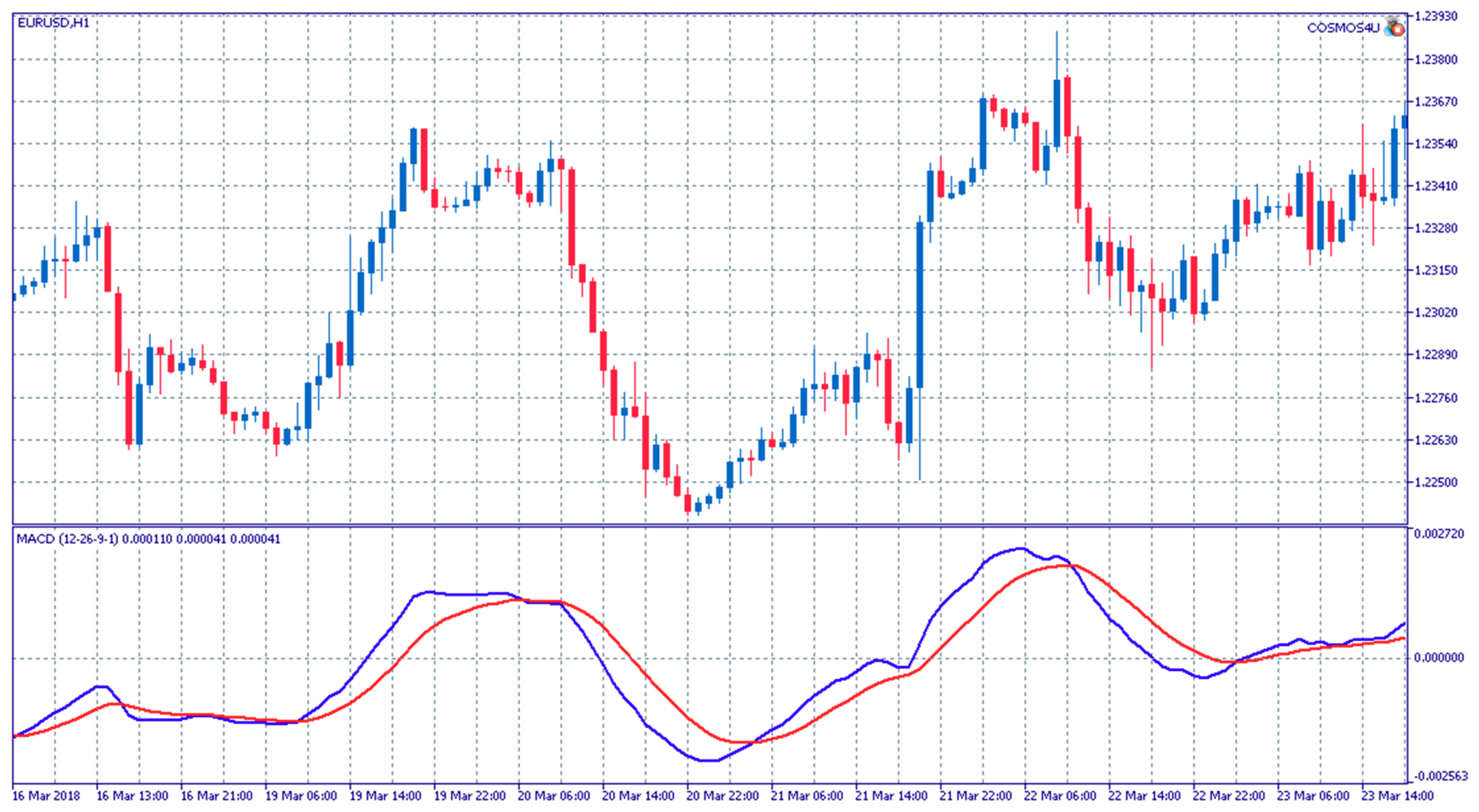
2.3.1. The MACD Indicator and Expert Advisor

The MACD (Moving Average Convergence/Divergence) is a well-known indicator created in 1979 by Appel (2005). It calculates the difference of two exponential moving averages of different periods over a time-series. The moving average with the smaller period is called the fast moving average and the moving average with the bigger period is called the slow moving average.
  MACD   line = EMA p f a s t ( Timeseries ) EMA p s l o w ( Timeseries ) , p f a s t < p s l o w  
Another exponential moving average is calculated on the MACD line, called the Signal line:
  Signal   line = EMA p s i g n a l ( MACD   line )  
When the MACD line is above the Signal line, this is an indication of an upward trend momentum in the time-series and when the MACD line is below the Signal line, this is an indication of a downward trend momentum in the time-series.
The default values of the three periods used in the calculations of the MACD indicator are usually p f a s t = 12 , p s l o w = 26 , and p s i g n a l = 9 in the daily timeframe. An example of the MACD indicator can be seen in Figure 1.
An automated trading system (Expert Advisor) can be formulated on the basis of the MACD indicator following the rules below:
When the MACD line crosses above the Signal line, this constitutes a buy signal and any short positions are closed and a long position is opened.
When the MACD line crosses below the Signal line, this constitutes a sell signal and any long positions are closed and a short position is opened.
The abovementioned trading strategy in the form of a pseudocode can be found in Appendix A.

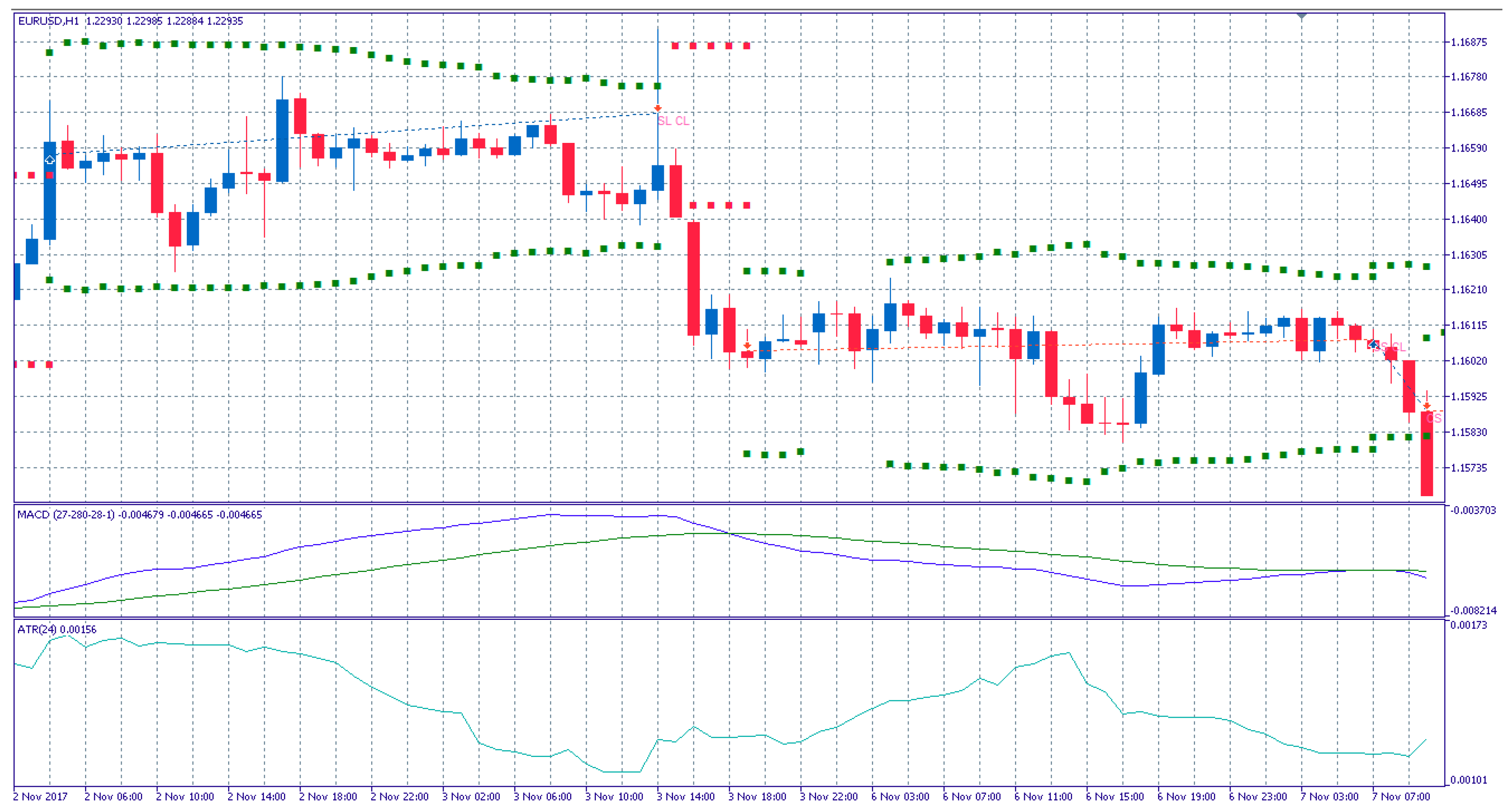
2.3.2. The MACD Expert Advisor with a quicker Take Profit Signal

Sometimes, the rate of change of a time-series can be more rapid than the rate at which the MACD indicator can provide us with a signal. If a position was open during that time, even if it was a successful one up until that moment, potential profits could be diminished and never materialize or even turn into losses.
A potential solution to that problem is the use of a different Signal line to judge when to exit a position, with a faster (smaller) period than that of the normal Signal line:
  Take   Profit   Signal   line = EMA p t a k e   p r o f i t   s i g n a l ( MACD   line )  
where
  p t a k e   p r o f i t   s i g n a l = p s i g n a l N , N = 2 ,   3 ,    
An example of the MACD indicator with a Take Profit Signal Line can be seen in Figure 2.
Now, the Expert Advisor, in addition to the two previous rules, closes any long positions when the MACD line crosses below the Take Profit Signal line and any short positions when the MACD line crosses above the Take Profit Signal line. After that and until the next time, the MACD line crosses the Signal line, and no position is open, in contrast with the previous strategy, where there was always a long or a short position open. The abovementioned trading strategy in the form of a pseudocode can be found in Appendix A.

2.3.3. The MACD Expert Advisor with Signal Lines’ Hierarchy

There can be time periods when the time-series of an asset does not follow a clear upward or downward trend, but instead oscillates around a value. During these periods, the previous strategies produce a lot of signals and change positions frequently, which can potentially lead to losses, because there is not enough time for the price to move to profitable levels and every transaction and position change comes at a cost. A more effective option might involve staying out of the market during these periods and only opening a new position when clear upward or downward trends occur.
The clarity of a trend can be judged by means of the MACD, Signal, and Take Profit Signal lines. When the prevailing trend is bullish, then we have the MACD line above the Take Profit Signal line and the Take Profit Signal line above the Signal line. Likewise, when the trend is bearish, we have the MACD line below the Take Profit Signal line and the Take Profit Signal line below the Signal line.
The Expert Advisor still closes positions using the Take Profit Signal line in the same way as in the previous case, but only opens new positions if the hierarchy of the MACD, Take Profit Signal, and Signal lines matches the one outlined in the above paragraph. The abovementioned trading strategy in the form of a pseudocode can also be found in Appendix A.

2.3.4. The Average True Range Indicator

The Average True Range or ATR indicator is a measure of volatility introduced in 1978 by Wilder (1978). The True Range for a specific interval is defined as
  TR = max [ ( high low ) ,   abs ( high close prev ) , abs ( low close prev ) ]  
The ATR of period N is calculated as
  ATR = 1 N i = 1 N TR i  
for the first instance and after that as
  ATR t = ATR t 1 × ( N 1 ) + TR t N  

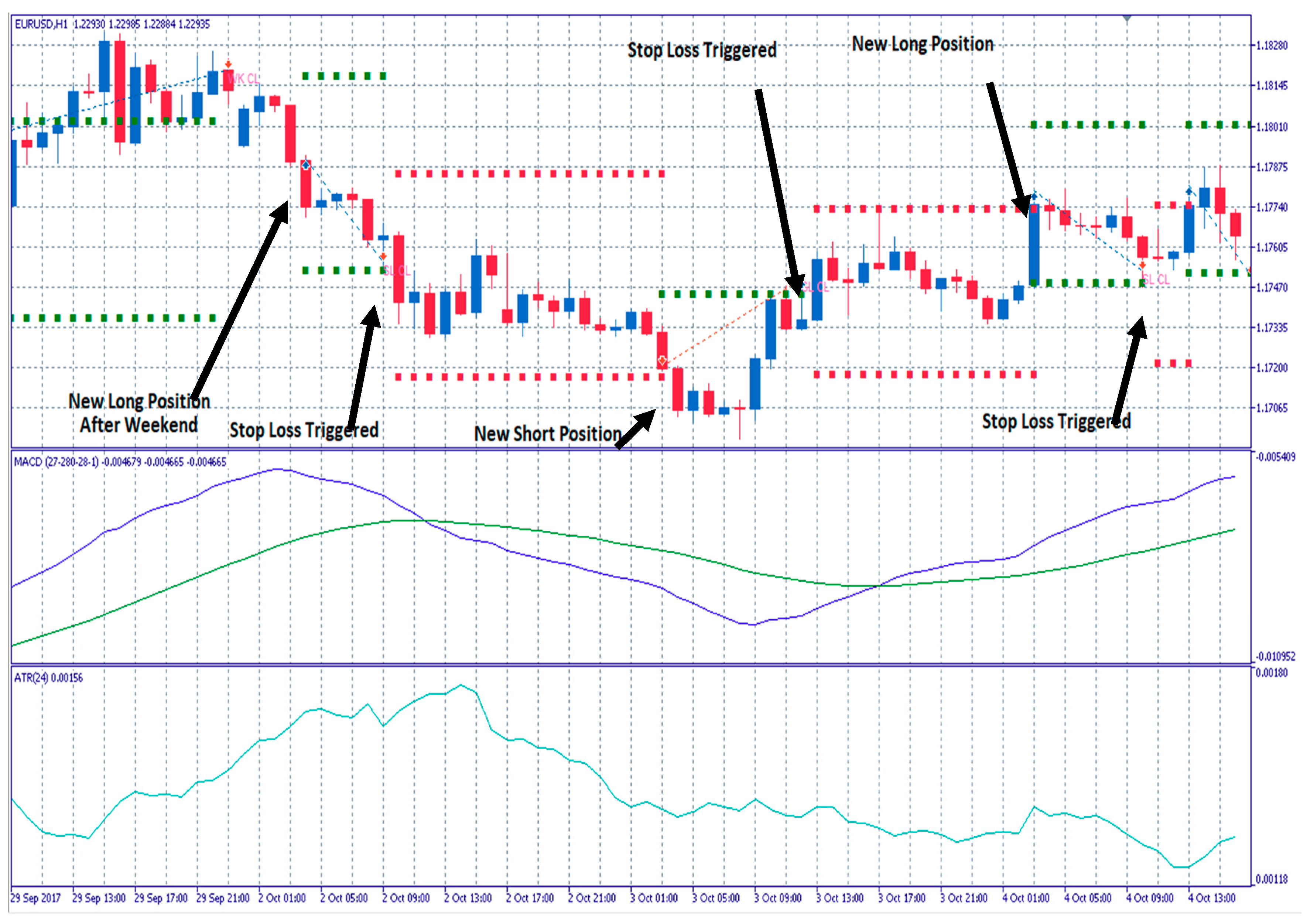
2.3.5. The MACD Expert Advisor combined with the ATR Indicator for Stop Loss Strategies

The ATR indicator can be used to set a Stop Loss barrier when a new position is opened following an MACD Expert Advisor signal. When the MACD Expert Advisor opens a new long position, a Stop Loss barrier can be set at
  Stop   Loss   Barrier = Opening   Price x × ATR ( N )  
where Opening Price is the price the long position was opened at, ATR(N) is the value of the ATR indicator of period N at that moment, and x is a constant multiplier used to adjust the barrier’s width. When the asset’s price moves below that barrier, the long position is closed.
Likewise, when a short position is opened, a Stop Loss barrier can be set at
  Stop   Loss   Barrier = Opening   Price + x × ATR ( N )  
When the asset’s price moves above this barrier, then the short position is closed.
After a Stop Loss is triggered and a position closed, it is possible that the MACD indicator keeps signaling for the same type of position to be opened. To avoid the immediate reopening of the same type of position after a Stop Loss, a new barrier can be created in the same way. Until the price moves above
  New   Position   Barrier = Closing   Price + y × ATR ( N )  
a long signal will not result in a new long position after a Stop Loss, and until the price moves below
  New   Position   Barrier = Closing   Price y × ATR ( N )  
a short signal will not result in a new short position after a Stop Loss. The y parameter is a constant multiplier used to adjust the barrier’s width, as is the case with x. Examples of Stop Loss Barriers and New Position Barriers can be seen in Figure 3. The abovementioned trading strategy in the form of a pseudocode can also be found in Appendix A.

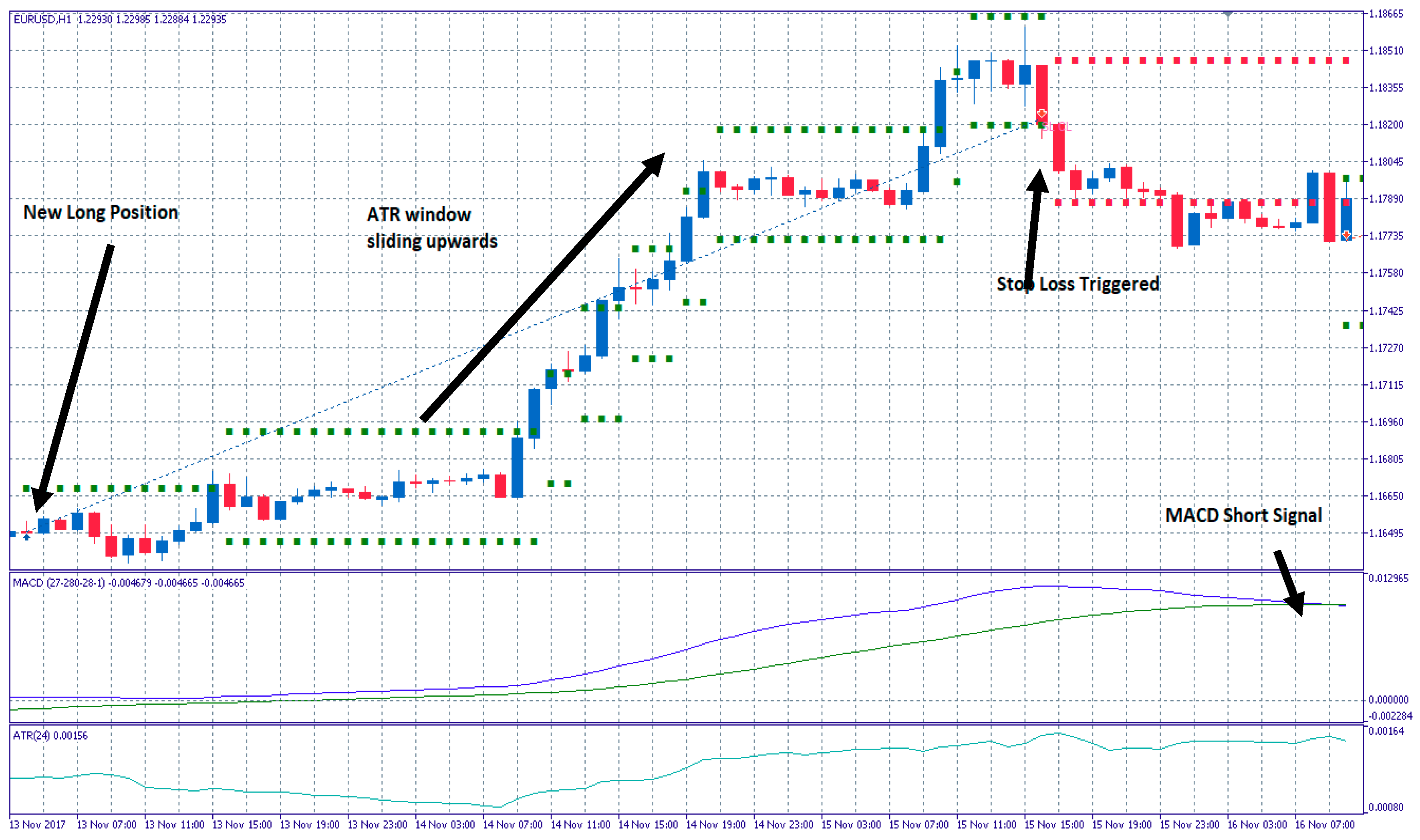
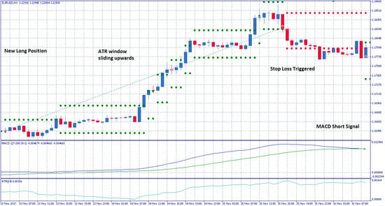
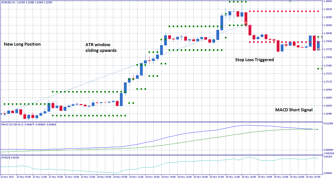
2.3.6. The MACD Expert Advisor with sliding ATR barrier zone

The ATR Stop Loss barriers described in the above section are drawn around the price at which a new position is opened and stay fixed, even if the price follows an upward, profitable trend, until there is a new MACD signal or the price moves back to the barrier.
In the second case, when the price moves back to the Stop Loss barrier, the potential gains from the previous profitable movements are never materialized. To prevent this, the ±x × ATR(N) zone can be redrawn each time the price moves out of it and follows a profitable direction. This slides the Stop Loss barrier to values that secure some of the profits gained so far.
On the other hand, the position prevention barrier should stay at the same level and not slide, as it could prevent the Expert Advisor from opening a new position for a long time. An example of this strategy can be seen in Figure 4.

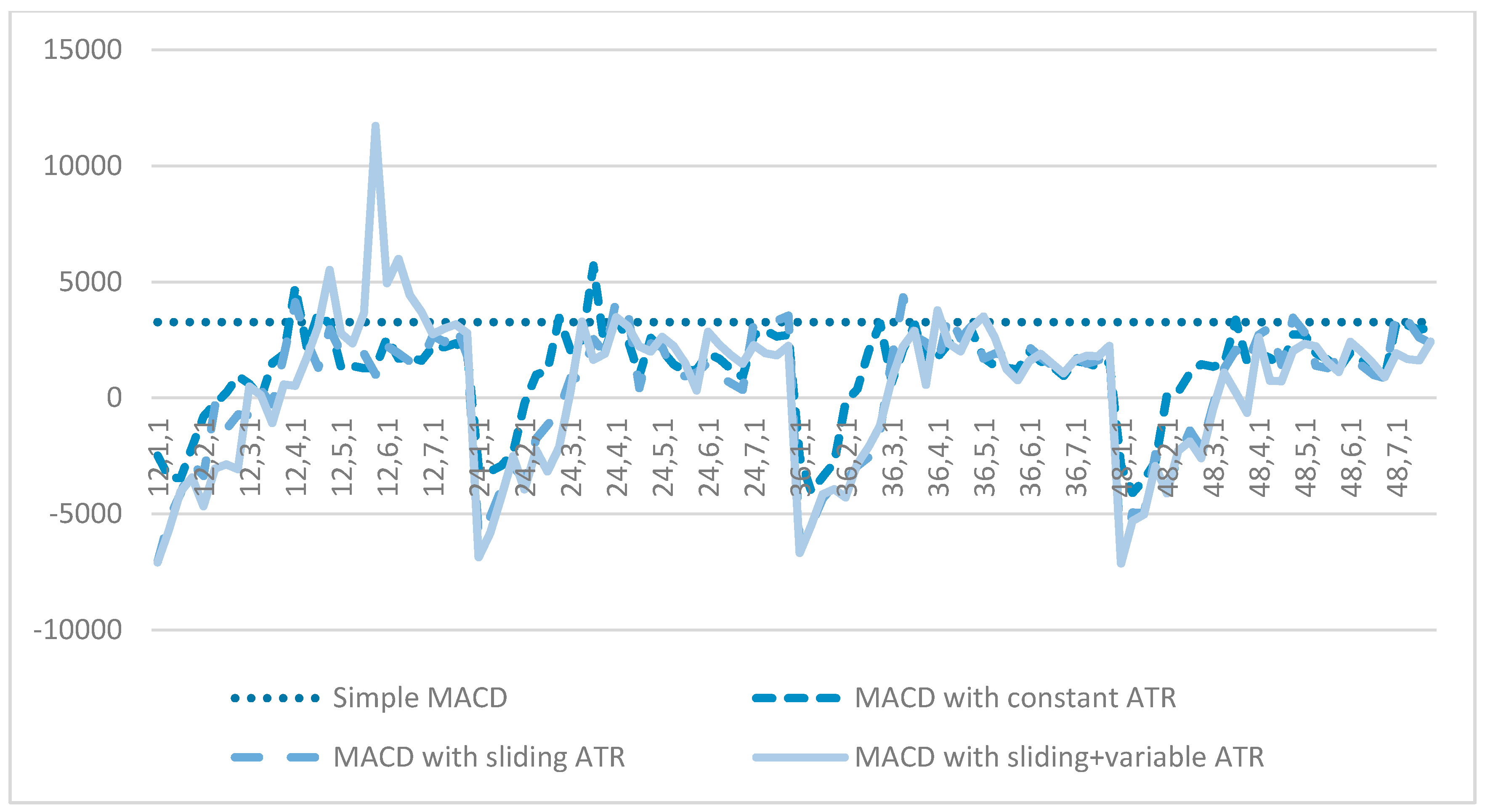
2.3.7. The MACD Expert Advisor with sliding and variable ATR barrier zone

An asset’s price can show large or small variability as it changes over time, which reflects the value of ATR. In the previous cases, ATR barriers were of a constant range, calculated with the ATR value at the moment when a position opened. Using the latest ATR value to form an ATR window with a variable range through time, could prevent the expert advisor from exiting a position prematurely in periods when variability spikes and help him follow the price trends, as seen in Figure 5.

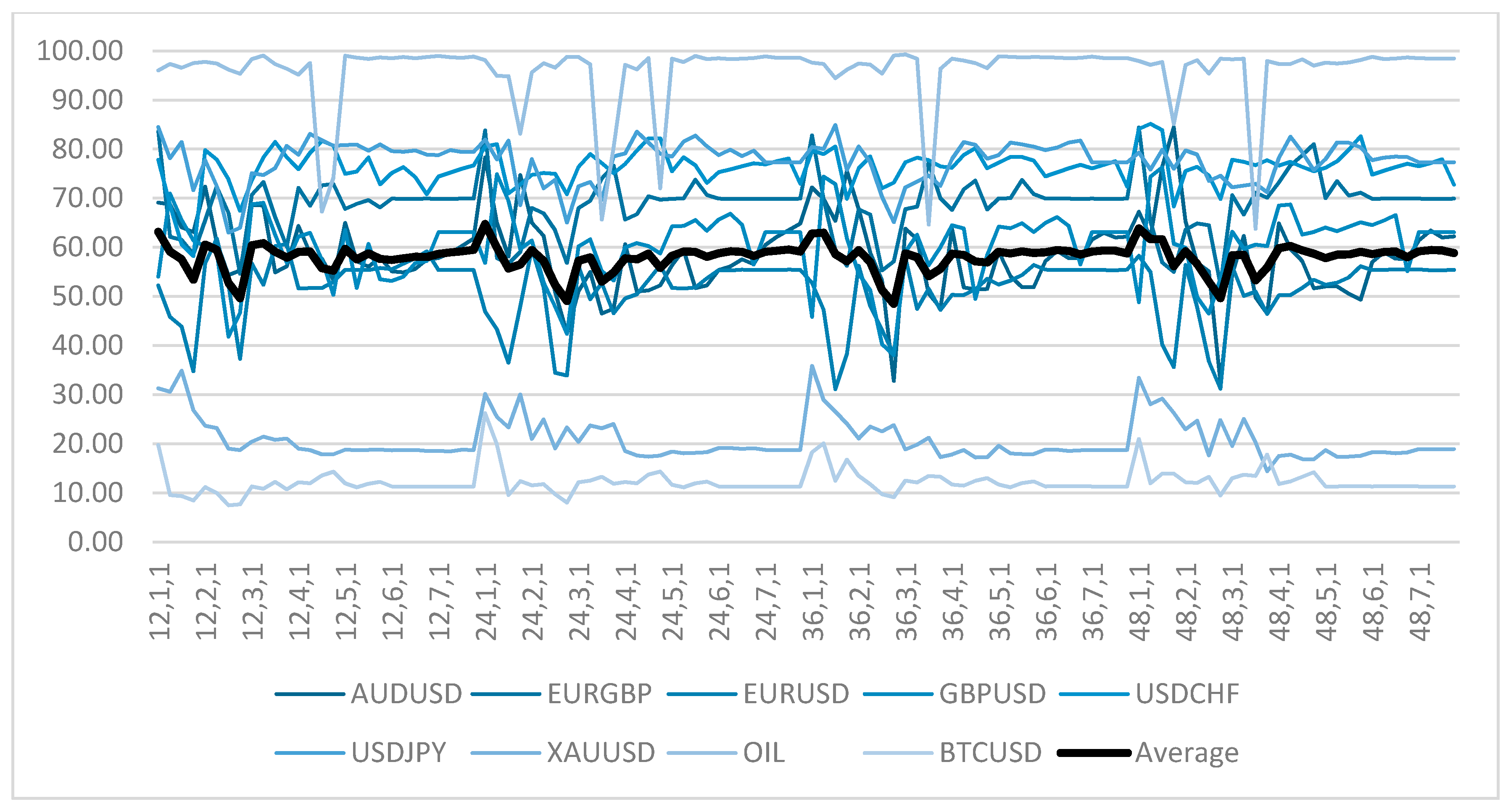
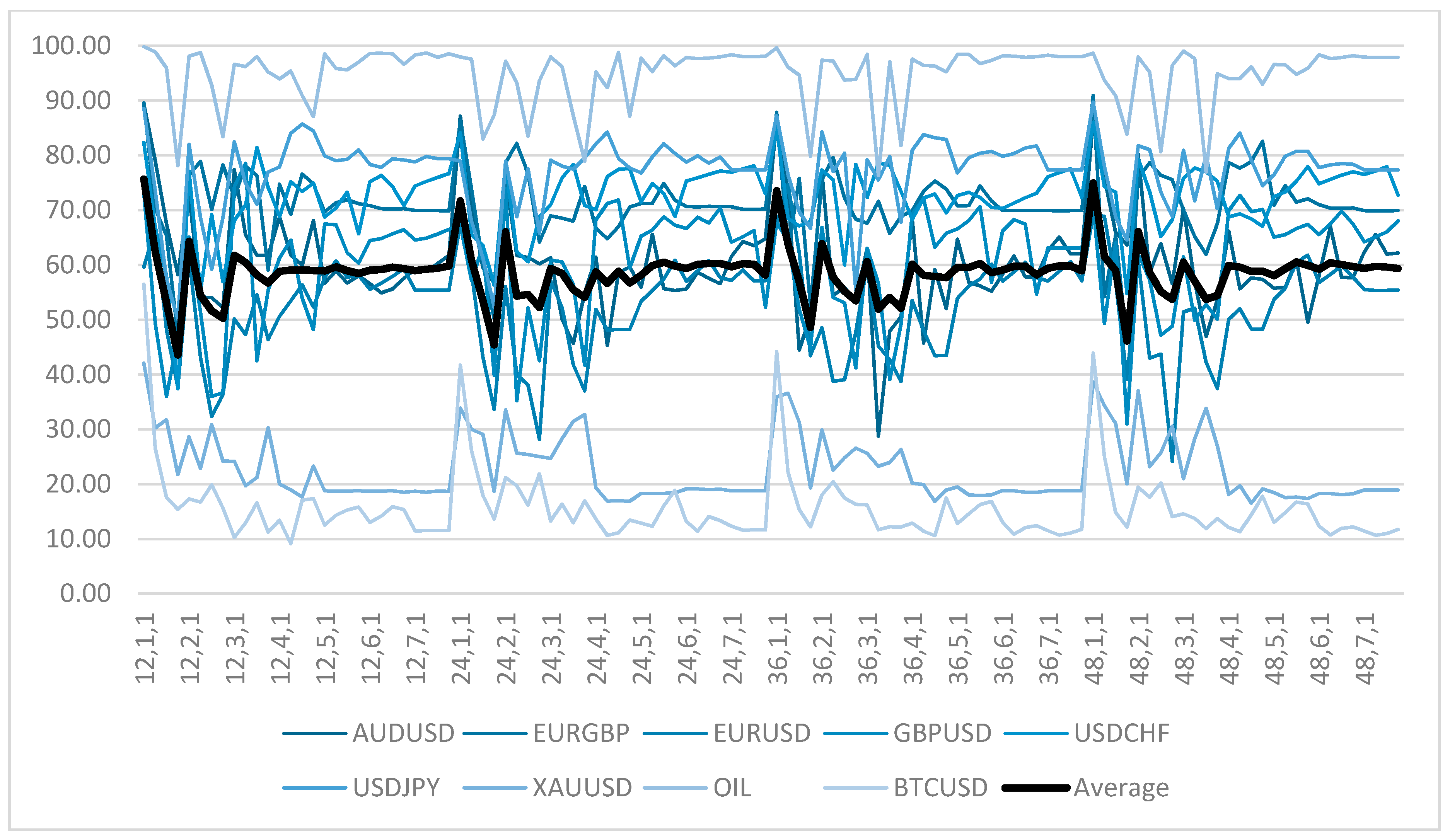
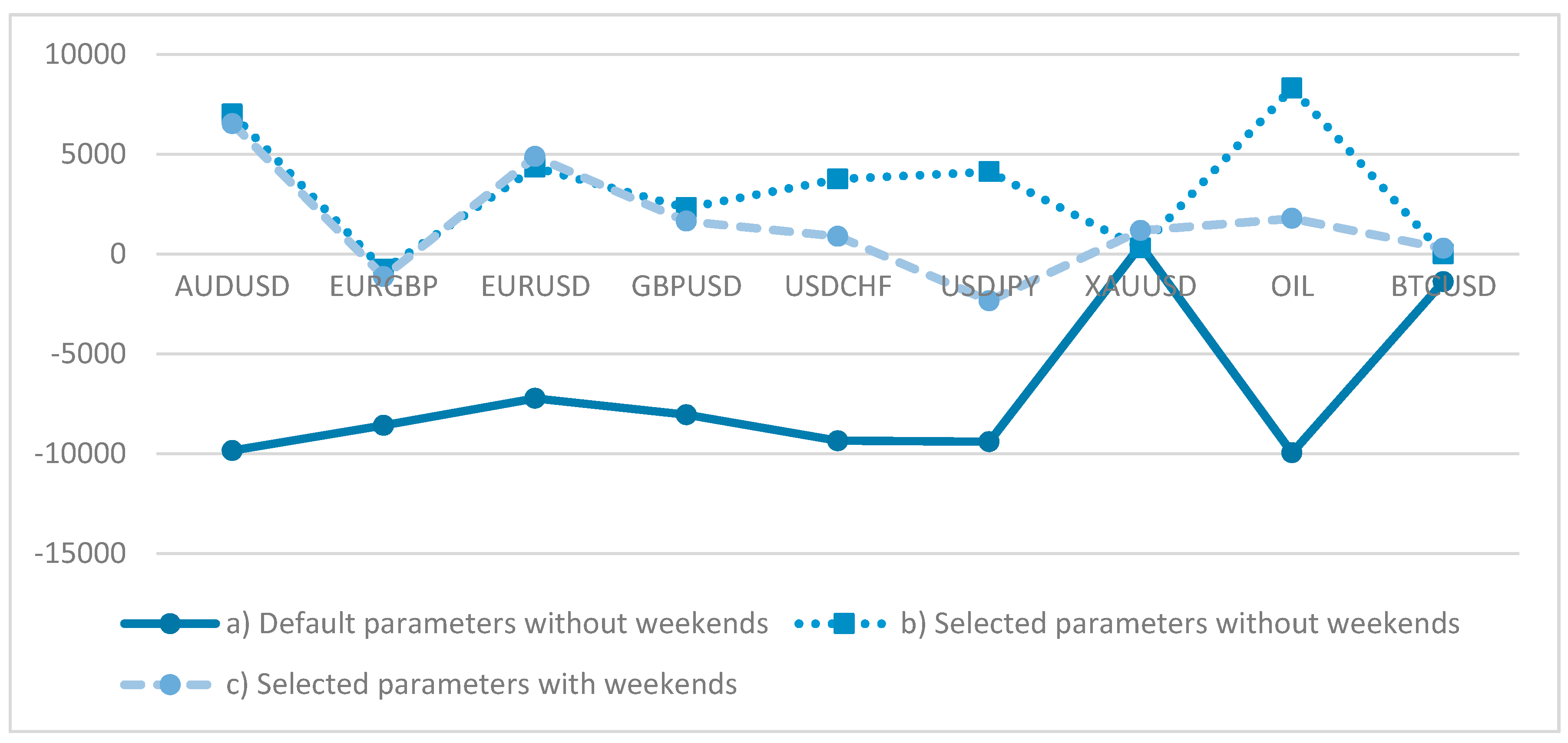
2.4. Data and Implementation

We conducted our experiments on the different Take Profit – Stop Loss strategies for nine assets from the Forex, Metals, Commodities, Energy, and Cryptocurrencies categories: AUDUSD, EURGBP, EURUSD, GBPUSD, USDCHF, USDJPY, XAUUSD, OIL, and BTCUSD. This choice mainly came from the need for assets that are traded on global markets on a 24 h base (or close to 24 h), as we wanted to examine the automated trading systems in a High Frequency Trading mode (hourly timeframe). The MACD Indicator has mainly been used for stock trading, but we opted to not trade stocks as the relatively big time intervals that exist between their trade sessions, in combination with the multinational activities of most of these corporations, can cause a lot of gaps and noise in their prices. The period we examined was from 3 September 2017 to 24 February 2018 with historical data from FXTM, GEBINVEST, and OctaFX. Because our systems were used in High Frequency Trading mode, we determined that a six-month period would be enough to draw conclusions about their performance.
For the testing, we used the Metatrader 5 trading terminal from Metaquotes, and Microsoft SQL Server for the initial data processing.
We set the initial test amount at $10,000 at a 1:100 leverage ratio for all assets except for BTCUSD, whose high price and spread required an equally high margin on the broker we used, so we set the initial amount at $10,000,000 and adjusted the results in such a way as to be comparable to the other assets. For each new position the automated trading system opens, it risks 20% of its current balance and no capital is deposited or withdrawn for the six-month period apart from the initial capital. The spreads for every asset (in pips) as reported by the brokers used were AUDUSD:0.7, EURGBP:0.6, EURUSD:0.4, GBPUSD:0.7, USDCHF:0.9, USDJPY:0.5, XAUUSD:21.0, OIL:5.0, and BTCUSD:11.5. The Metatrader 5 trading terminal also automatically adds the cost of each transaction to the Gross Losses so the Net Profits represent the actual pure number a trader has won or lost at the end.

2.4.1. Back testing Limitations

The Metatrader 5 terminal offers the ability to test an automated trading system over a past time period with various methods for simulating the price changes, such as every tick, every open-high-low-close value, every open value for a specific timeframe, etc. It also offers the ability to test a rage of the parameters used by the Expert Advisor in order to identify the best combination of parameters for a back testing period. In order to speed up back-tests, Metatrader 5 also offers the ability to use distributed testing agents utilizing the resources of a local network of computers. We used this ability to form a local cluster of computers, mainly with i5, i7, and Xeon Intel CPUs for a total capacity of 130 distributed agents, in order to run our backtesting experiments. We also used a Microsoft SQL Server in order to save and process the results of our experiments during the stage of parameter selection.
It should be noted that the wider the parameters’ ranges, the greater the number of combinations of parameters. Also, back testing with an every tick simulation is far more time- and resource-consuming than back testing with open-high-low-close value, which is in turn more time-consuming than an open value only simulation.
The values of the MACD and ATR indicators are calculated over one-hour timeframes, but during an hourly timeframe, the price of an asset can reach levels that would trigger a Take Profit/Stop Loss in some strategies or an automatic Stop Loss from the broker, so we chose to run our experiments with every tick simulations.

2.4.2. Parameter Selection

For our tests, we had to choose a set of parameters for each asset that would allow for the demonstration of an improvement or worsening in the MACD Expert Advisor’s behavior with the introduction of each Take Profit/Stop Loss strategy.
Since the different periods in the MACD averages can generate widely different results and in order to render the role of these parameters less significant for our tests, we decided to choose sets of parameters that are centered on neighborhoods (±2) of similar results, with the results indicating there is room for both improvement and worsening.
The simple MACD Expert Advisor has three parameters, the periods of its moving averages, which means that even for small parameter ranges, the number of combinations is significant. Performing a back test for every asset with full parameter sweeping on an every tick simulation would be prohibitive because of the time and electrical energy it would require. We circumvented this firstly by running the simulations on open-high-low-close prices ticks, which produces results close enough to the real tick simulation, and secondly by incrementing each parameter by a step of 2 instead of 1, which reduces the combinations to 1/8, allowing us to check a wider range. Potentially suitable neighborhoods can still be identified as a step of 2 still hits a ±2 neighborhood in eight or 27 of its 125 members.
Next, we defined some requirements for a suitable neighborhood, such as a minimum amount of trades and profit range, and chose the best 100 neighborhoods that fulfilled them, sorted by the smallest relative range defined as
  Relative   Range = max ( Profits ) min ( Profits ) average ( Profits )  
The specific requirements for each asset can be seen in Table 1.
To be more certain, we ran back tests with every tick value for these 100 neighborhoods of each asset, with range ±2 around their center with step 1. The missing combinations changed the min, max and average profits of the neighborhoods, which resulted in changes in their order of classification. Finally, we conducted a supervisory review of the best options and chose a neighborhood for each asset that seemed the most fitting one and served our purposes. The final parameters are presented in Table 2.

3. Results and Discussion

3.1. Default/Selected Parameters and Weekends

Firstly, we compared the results for a) the simple MACD Expert Advisor with the default parameters p f a s t = 12 , p s l o w = 26 , and p s i g n a l = 9 and without holding positions over weekends; b) the simple MACD Expert Advisor with our selected parameters and without holding positions over weekends; and c) the simple MACD Expert Advisor with our selected parameters with holding open positions over the weekends. Although the default MACD parameters refer to the daily timeframe, attempting to express two weeks, one month, and 1.5 weeks, respectively, we opted to keep them the same in the hourly timeframe instead of using the equivalent p f a s t = 288 , p s l o w = 624 , and p s i g n a l = 216 of days expressed in hours since that would move the scale outside the HFT. By porting the default parameters to the hourly timeframe, they then expressed ½ of a day, one day, and one work-day, which is closer to the timeframe of a daily trader doing HFT. The results of these three experiments can be seen in Table A1 and Table A2 and Figure 6 and Figure 7.
It can be concluded that holding open positions over the weekends helps cut one’s losses, but it also takes away a proportion of the profits for all the examined assets. Figure 6 makes clear that the net profits in most cases are diminished and Figure 7 shows the usually higher drawdown when holding positions open over the weekend. Also, using the default parameters almost always results in losses. Because of differences in contract sizes, trading hours, variability, etc., the XAUUSD, OIL, and BTCUSD show different numbers compared with the FOREX pairs (a behavior that also presents itself to the rest of the experiments) but, in the relativity of the experiments’ comparisons, their numbers still support the conclusions. The Net Profits in Table A1 and, by extension, for all later experiments, are a result of the parameter selection described in Section 2.4.2., which is a posteriori process. The actual amount of returns and the profitability of the MACD Expert Advisor are not something we actually concern ourselves with in this research, but rather how these returns change by adding each Take Profit and Stop Loss strategy.
From now on, in our experiments, we will be using our selected parameters for each asset and open positions will be closed for the weekends.

3.2. Fast Take Profit Signal and Signals’ Hierarchy

Next, we compared the (b) simple MACD Expert Advisor with the (d) MACD Expert Advisor, with the addition of a faster take profit signal, as described in Section 2.3.2. The determined value of the divisor N of the Fast Signal period was set as follows: N = {2,3,4}. With N = 1, the (d) Expert Advisor effectively becomes the same as (b), as the Fast Signal line becomes identical to the Signal line. Their results can be seen in Table A3 and Table A4 and Figure 8 and Figure 9.
The simple MACD yields better results in most cases, both in terms of net profits and drawdown, especially on Forex pairs. Even when assets which are traded using the MACD do not yield the most profitable results, it is postulated that the MACD ranks second after a neck-and-neck round, with a fast Take Profit signal of N = 2.
Next, we compared the (b) simple MACD Expert Advisor with the (e) MACD Expert Advisor that only opens new positions when the hierarchy of the MACD and Signal lines is right, as described in Section 2.3.3. The divisor N of the Fast Signal period assumed values of N = {2,3,4}. With N = 1, the e) Expert Advisor becomes the same as (b). Their results can be seen in Table A5 and Table A6 and Figure 10 and Figure 11.
Again, it is evident that the simple MACD Expert Advisor generally produces better results than the MACD, which opens positions with the hierarchy of lines.

3.3. Constant ATR Zone, Sliding ATR Zone, Sliding and Variable ATR Zone

The first Stop Loss strategy we examined was f) a MACD Expert Advisor that creates a Stop Loss zone at ±x × ATR(N) when it opens a new position and a new position prevention zone at ±y × ATR(N), after a position has to be closed due to a Stop Loss that has been triggered. We tested every combination of parameters for N:{12,24,36,48}, x:{1,2,3,4,5,6,7}, and y:{1,2,3,4}. The Net Profits for each asset for every combination of N, x, y have been outlined in Figure 12 and Drawdown in Figure 13.
The periodicity that can be seen in Figure 12 indicates that the x multiplier plays a significant role in this strategy. For small values of x (=1), net profits are diminished for all assets, while with larger values of x (5,6,7), profits are more constant and approach those of the simple MACD, as the big ATR zone does not trigger a Stop Loss very often. Values of x (2,3,4) yield the best results compared to the others. In the drawdown diagram, there also seems to be periodicity for y, with bigger values (y = 3,4) having lower drawdown.
Next, we examined g) an MACD Expert Advisor with a sliding Stop Loss zone ±x × ATR(N) as described in Section 2.3.6 and a constant new position prevention zone at ±y × ATR(N). We tested every combination of parameters for N:{12,24,36,48}, x:{1,2,3,4,5,6,7}, and y:{1,2,3,4}. The Net Profits for each asset for every combination of N, x, y are displayed in Figure 14 and Drawdown in Figure 15.
The general picture is the same as the case of (f). For small values of x, the profits are diminished, while for larger values of x, they tend to stay constant and approach the Simple MACD’s results. Additionally, large values of y tend to have lower drawdown.
Finally, we examined (h) an MACD Expert Advisor with a sliding and variable Stop Loss zone ±x × ATR(N), with a new value of ATR used at hourly intervals as described in Section 2.3.7 and a constant new position prevention zone at ±y × ATR(N). We tested every combination of parameters for N:{12,24,36,48}, x:{1,2,3,4,5,6,7}, and y:{1,2,3,4}. The Net Profits for each asset for every combination of N, x, y have been outlined in Figure 16 and Drawdown in Figure 17.
In this case, apart from the same conclusions that can be reached in the two previous tests, we can observe a clear peak in the profits in the neighborhood of (12,6,2), even when accounting for the big spikes from the OIL profits (the drawdown is also below total average in this area). This becomes more evident when we draw the diagram, Figure 18, of average profits for the (b) Simple MACD, (f) MACD with a constant ATR zone, (g) MACD with a sliding ATR zone, and (h) MACD with a sliding and variable ATR zone.
A neighborhood around 12,6,2 of MACD with sliding and variable ATR windows clearly stands out, consistently having the edge over the simple MACD, as well as the other Stop Loss strategies. Apart from some solitary peaks, the other strategies do not outperform the simple MACD system.

4. Conclusions

In the present research, we examined various Take Profit and Stop Loss strategies added to a simple MACD automated trading system used in trading 10 assets from the Forex, Metals, Energy, and Cryptocurrencies categories. In order to make the MACD parameters less important in our research, we chose parameters based on the characteristics of their neighborhoods of ±2 and used them for all our experiments.
In our research, we first of all concluded that it is generally less profitable to keep positions open during weekends. Another conclusion we reached is that Take Profit strategies based on faster take profit signals on MACD are not far better than a simple MACD strategy. We also showed that among the different Stop Loss strategies based on ATR windows, the best and safest results come from a sliding and variable ±x × ATR(N) window with period N = 12 and multiplier x = 6 after opening a position and a constant ±y × ATR(N) with period N = 12 and multiplier y = 2 after stop loss closing.
Since the MACD Indicator is used quite prevalently by a lot of traders and our results are general enough, a trader could incorporate them in their technical analysis/trading strategy for Stop Loss and Take Profit without interfering with the rest of their strategy (portfolio management, capital allocation, MACD parameter selection, etc.)

Author Contributions

Conceptualization, D.V.; Investigation, D.V.; Methodology, D.V.; Software, T.K.; Supervision, C.S.; Visualization, T.K.

Funding

This research has been co-financed by the European Union and Greek national funds through the Operational Program Competitiveness, Entrepreneurship and Innovation, under the call RESEARCH—CREATE—INNOVATE (project code:T1EDK-02342).

Acknowledgments

We would like to thank COSMOS4U for providing the infrastructure used to conduct this research. We would also like to thank the anonymous referees who reviewed our paper and provided us with valuable insights and suggestions.

Conflicts of Interest

The authors declare no conflict of interest. The funders had no role in the design of the study; in the collection, analyses, or interpretation of data; in the writing of the manuscript, and in the decision to publish the results.

Appendix A

Pseudocode of the basic MACD trading strategy as described in Section 2.3.1. Jrfm 11 00056 i001
Pseudocode of the MACD trading strategy with a faster Take Profit Signal, as described in Section 2.3.2. Jrfm 11 00056 i002
Pseudocode of the MACD trading strategy using the Signal Lines’ Hierarchy, as described in Section 2.3.3. Jrfm 11 00056 i003
Pseudocode of the MACD trading strategy with a constant ATR Stop Loss barrier zone, as described in Section 2.3.5. Jrfm 11 00056 i004

Appendix B

Table A1. Results of experiments (a), (b), and (c).
Gross ProfitsGross LossesNet Profits
abcabcabc
AUDUSD13,966.2437,297.7831,166.56−23,816.08−30,282.34−24,627.67−9849.847015.446538.89
EURGBP22,526.9454,321.3949,798.47−31,113.62−55,099.62−50,929.09−8586.68−778.23−1130.62
EURUSD45,671.4836,106.5932,522.98−52,901.34−31,757.62−27,630.16−7229.864348.974892.82
GBPUSD56,474.1148,025.8644,737.63−64,529.80−45,705.37−43,091.59−8055.692320.491646.04
USDCHF18,662.6427,822.3219,855.93−28,019.51−24,060.67−18,962.81−9356.873761.65893.12
USDJPY20,697.0227,060.2314,940.23−30,106.48−22,931.07−17,282.76−9409.464129.16−2342.53
XAUUSD17,208.719107.399749.19−16,773.68−8800.84−8564.85435.03306.551184.34
OIL9098.1881,584.5857,452.95−19,058.36−73,261.17−55,665.34−9960.188323.411787.61
BTCUSD3297.662410.972462.69−4681.72−2404.57−2175.06−1384.056.40287.62
Table A2. Additional results of experiments (a), (b), and (c).
DrawdownTrades
abcabc
AUDUSD98.7952.9048.822665940
EURGBP91.6266.8267.88242162141
EURUSD82.5147.9542.182438160
GBPUSD90.0355.7859.42248152133
USDCHF94.5673.4072.922548364
USDJPY96.8073.3679.952408669
XAUUSD27.3216.4016.0422811999
OIL99.6098.4398.071888059
BTCUSD14.459.449.502218464
Table A3. Results of experiment (d) for various values of N.
Gross ProfitsGross LossesNet Profits
b (N = 1)d, N = 2d, N = 3d, N = 4b (N = 1)d, N = 2d, N = 3d, N = 4b (N = 1)d, N = 2d, N = 3d, N = 4
AUDUSD37,29425,47424,725544−30,278−25,896−24,269−297015−422456515
EURGBP54,41559,52055,50355,503−55,194−60,383−58,596−58,596−778−863−3094−3094
EURUSD36,11637,64238,38940,268−31,767−32,361−33,461−37,0114349528149293257
GBPUSD47,99948,22054,56647,588−45,679−47,279−54,533−49,227232094133−1639
USDCHF27,82920,63418,82120,256−24,067−22,316−21,671−22,7523762−1683−2850−2496
USDJPY27,05621,23326,47526,142−22,927−23,304−26,338−27,9424129−2072137−1799
XAUUSD9115904898649928−8809−8618−8476−891230743013881016
OIL81,59371,42151,23651,994−73,269−66,204−56,279−58,57883235217−5043−6584
BTCUSD2377224722842265−2371−2554−2586−25766−307−302−311
Table A4. Additional results of experiment (d) for various values of N.
DrawdownTrades
b (N = 1)d, N = 2d, N = 3d, N = 4b (N = 1)d, N = 2d, N = 3d, N = 4
AUDUSD59.8473.9269.7265.1359676874
EURGBP70.0373.4976.1476.14162186210210
EURUSD55.4457.4856.3357.82818896104
GBPUSD52.1363.1658.4761.14152171192216
USDCHF74.9875.6078.3575.7083101112118
USDJPY77.0683.0478.2478.2186101104112
XAUUSD18.7313.4710.7811.96119136152161
OIL98.8097.8098.1497.3580879399
BTCUSD11.3013.8113.4212.84848996105
Table A5. Results of experiment (e) for various values of N.
Gross ProfitsGross LossesNet Profits
b (N = 1)e, N = 2e, N = 3e, N = 4b (N = 1)e, N = 2e, N = 3e, N = 4b (N = 1)e, N = 2e, N = 3e, N = 4
AUDUSD37,29424,83826,66629,074−30,278−23,346−22,296−26,1207015149243702954
EURGBP54,41536,83644,97444,974−55,194−41,263−49,168−49,168−778−4428−4194−4194
EURUSD36,11628,17235,25237,813−31,767−25,534−30,184−33,6214349263850684192
GBPUSD47,99939,27449,65751,052−45,679−40,010−48,985−51,9982320−736671−946
USDCHF27,82915,94916,94117,136−24,067−20,830−21,086−21,1713762−4880−4146−4035
USDJPY27,05617,32823,07625,002−22,927−20,258−24,040−27,3394129−2929−964−2338
XAUUSD9115722078828678−8809−7950−7623−8112307−730259566
OIL81,59384,18274,12559,685−73,269−72,111−72,253−65,487832312,0711871−5802
BTCUSD2377208522082179−2371−2171−2476−25126−86−267−333
Table A6. Additional results of experiment (e) for various values of N.
DrawdownTrades
b (N = 1)e, N = 2e, N = 3e, N = 4b (N = 1)e, N = 2e, N = 3e, N = 4
AUDUSD59.8468.6860.7157.7259636571
EURGBP70.0372.4575.0175.01162175205205
EURUSD55.4451.9847.6852.07817791100
GBPUSD52.1362.4557.6363.58152153178206
USDCHF74.9880.7179.2878.968397109115
USDJPY77.0684.7379.4477.03869297105
XAUUSD18.7322.3519.3915.90119124143153
OIL98.8095.6795.3297.0580768591
BTCUSD11.3012.0012.8513.20848091102

References

  1. Appel, Gerald. 2005. Technical Analysis: Power Tools for Active Investors. Upper Saddle River: FT Press. [Google Scholar]
  2. Au, Kevin, Forrest Chan, Denis Wang, and Ilan Vertinsky. 2003. Mood in foreign exchange trading: Cognitive processes and performance. Organizational Behavior and Human Decision Processes 91: 322–38. [Google Scholar] [CrossRef]
  3. Austin, Mark P., Graham Bates, Michael AH Dempster, Vasco Leemans, and Stacy N. Williams. 2004. Adaptive systems for foreign exchange trading. Quantitative Finance 4: 37–45. [Google Scholar] [CrossRef]
  4. Azzini, Antonia, and Andrea GB Tettamanzi. 2008a. Evolving neural networks for static single-position automated trading. Journal of Artificial Evolution and Applications, 17. [Google Scholar] [CrossRef]
  5. Azzini, Antonia, and Andrea GB Tettamanzi. 2008b. Evolutionary single-position automated trading. In Workshops on Applications of Evolutionary Computation. Berlin/Heidelberg: Springer. [Google Scholar]
  6. Barbosa, Rui Pedro, and Orlando Belo. 2010. Multi-Agent Forex Trading System. In Agent and Multi-agent Technology for Internet and Enterprise Systems. Berlin: Springer, vol. 289, pp. 91–118. [Google Scholar]
  7. Bates, R. Graham, Michael AH Dempster, and Yazann S. Romahi. 2003. Evolutionary reinforcement learning in FX order book and order flow analysis. Paper presented at IEEE International Conference on Computational Intelligence for Financial Engineering, Hong Kong, China, March 20–23. [Google Scholar]
  8. Bolgün, Kaan Evren, Engin Kurun, and Serhat Güven. 2010. Dynamic Pairs Trading Strategy for the Companies Listed in the Istanbul Stock. International Review of Applied Financial Issues and Economics 2: 37. [Google Scholar] [CrossRef] [Green Version]
  9. Barber, Brad M., Yi-Tsung Lee, Yu-Jane Liu, and Terrance Odean. 2008. Just how much do individual investors lose by trading? The Review of Financial Studies 22: 609–32. [Google Scholar] [CrossRef]
  10. Brogaard, Jonathan, Terrence Hendershott, and Ryan Riordan. 2014. High-frequency trading and price discovery. The Review of Financial Studies 27: 2267–306. [Google Scholar] [CrossRef]
  11. Osler, Carol L. 2005. Stop-loss orders and price cascades in currency markets. Journal of International Money and Finance 24: 219–41. [Google Scholar] [CrossRef]
  12. Cervelló-Royo, Roberto, Francisco Guijarro, and Karolina Michniuk. 2015. Stock market trading rule based on pattern recognition and technical analysis: Forecasting the DJIA index with intraday data. Expert Systems with Applications 42: 5963–75. [Google Scholar] [CrossRef]
  13. Chaboud, Alain P., Benjamin Chiquoine, Erik Hjalmarsson, and Clara Vega. 2014. Rise of the machines: Algorithmic trading in the foreign exchange market. The Journal of Finance 69: 2045–84. [Google Scholar] [CrossRef]
  14. Challet, Damien, and Ahmed Bel Hadj Ayed. 2014. Do Google Trend data contain more predictability than price returns? Available online: https://arxiv.org/abs/1403.1715 (accessed on 24 July 2018).
  15. Chan, Oliver, and Alfred Ka Chun Ma. 2015. A Framework for Stop-Loss Analysis on Trading Strategies. The Journal of Trading 10: 87–95. [Google Scholar] [CrossRef]
  16. Chevallier, Julien, Wei Ding, and Florian Ielpo. 2012. Implementing a Simple Rule for Dynamic Stop-Loss Strategies. The Journal of Investing 21: 111–14. [Google Scholar] [CrossRef]
  17. Chong, Terence Tai-Leung, and Wing-Kam Ng. 2008. Technical analysis and the London stock exchange: testing the MACD and RSI rules using the FT30. Applied Economics Letters 15: 1111–14. [Google Scholar] [CrossRef]
  18. Clare, Andrew, James Seaton, Peter N. Smith, and Stephen Thomas. 2013. Breaking into the blackbox: Trend following, stop losses and the frequency of trading–The case of the S&P500. Journal of Asset Management 14: 182–94. [Google Scholar]
  19. Easley, David, MM Lopez De Prado, and Maureen O’Hara. 2011. The microstructure of the flash crash: Flow toxicity, liquidity crashes and the probability of informed trading. Journal of Portfolio Management 37: 118–28. [Google Scholar] [CrossRef]
  20. Foucault, Thierry, Bruno Biais, and Sophie Moinas. 2011. Equilibrium High Frequency Trading. Paper presented at International Conference of the French Finance Association, Montpellier, France, May 11. [Google Scholar]
  21. Han, Yufeng, Guofu Zhou, and Yingzi Zhu. 2016. Taming Momentum Crashes: A Simple Stop-Loss Strategy. Available online: https://ssrn.com/abstract=2407199 or http://dx.doi.org/10.2139/ssrn.2407199 (accessed on 26 July 2018).
  22. Hendershott, Terrence, Charles M. Jones, and Albert J. Menkveld. 2011. Does algorithmic trading improve liquidity? The Journal of Finance 66: 1–33. [Google Scholar] [CrossRef]
  23. Hendershott, Terrence, and Pam Moulton. 2007. The Shrinking New York Stock Exchange Floor and the Hybrid Market. Technical Report. Berkeley: University of California, Available online: https://docplayer.net/13539804-The-shrinking-new-york-stock-exchange-floor-and-the-hybrid-market.html (accessed on 25 July 2018).
  24. Jain, Pankaj K. 2005. Financial market design and the equity premium: Electronic versus floor trading. The Journal of Finance 60: 2955–85. [Google Scholar] [CrossRef]
  25. Kaminski, Kathryn, and Andrew W. Lo. 2014. When do stop-loss rules stop losses? Journal of Financial Markets 18: 234–54. [Google Scholar] [CrossRef]
  26. Kaniel, Ron, Saar Gideon, and Titman Sheridan. 2004. Individual Investor Sentiment and Stock Returns. Available online: https://ssrn.com/abstract=1294447 (accessed on 24 July 2018).
  27. Klement, Joachim. 2013. Assessing Stop-Loss and Re-Entry Strategies. Available online: https://ssrn.com/abstract=2277722 or http://dx.doi.org/10.2139/ssrn.2277722 (accessed on 26 July 2018).
  28. Lei, Adam YC, and Huihua Li. 2009. The Value of Stop Loss Strategies. Financial Services Review 18: 23–51. [Google Scholar] [CrossRef]
  29. Leung, Tim, and Xin Li. 2015. Optimal mean reversion trading with transaction costs and stop-loss exit. International Journal of Theoretical and Applied Finance 18: 1550020. [Google Scholar] [CrossRef]
  30. Martinez, Leonardo C., Diego N. da Hora, Joao R. de M. Palotti, Wagner Meira, and Gisele L. Pappa. 2009. From an artificial neural network to a stock market day-trading system: A case study on the BM&F BOVESPA. Paper presented at International Joint Conference on Neural Networks, Atlanta, GA, USA, June 14–19. [Google Scholar]
  31. Ni, He, and Hujun Yin. 2009. Exchange rate prediction using hybrid neural networks and trading indicators. Neurocomputing 72: 2815–23. [Google Scholar] [CrossRef]
  32. Preis, Tobias, Helen Susannah Moat, and H. Eugene Stanley. 2013. Quantifying trading behavior in financial markets using Google Trends. Scientific Reports 3: 1684. [Google Scholar] [CrossRef] [PubMed]
  33. Krishnan, Rajeswari, and S. Sandhya Menon. 2009. Impact of Currency Pairs, Time Frames and Technical Indicators on Trading Profit in Forex Spot Market. International Journal of Business Insights & Transformation 2: 34–51. [Google Scholar]
  34. Wilder, J. Welles. 1978. New Concepts in Technical Trading Systems. Chicago: Investor Publishing, Inc. [Google Scholar]
  35. Yazdi, Seyed Hadi Mir, and Ziba Habibi Lashkari. 2013. Technical Analysis of Forex by MACD Indicator. International Journal of Humanities and Management Sciences 1: 159–65. [Google Scholar]
Figure 1. EURUSD chart with an MACD line (blue) and a Signal line (red) below.
Jrfm 11 00056 g001
Figure 2. EURUSD chart with an MACD line (blue), a Signal line (red), and a Take Profit Signal line (green) below.
Jrfm 11 00056 g002
Figure 3. A segment from an MACD Expert Advisor’s trading on EURUSD. The green dots on the price chart indicate the ±2 × ATR(24) Stop Loss barrier after opening a new position and the red dots indicate the ±2 × ATR(24) barrier for new positions prevention after Stop Loss.
Jrfm 11 00056 g003
Figure 4. A segment from an MACD Expert Advisor’s trading on EURUSD. The green dots show how the ±2 × ATR(24) zone slides upwards as the price moves to more profitable values. Eventually, a stop loss is triggered and the position is closed at a higher price than the one we would have in the event of waiting for the next MACD signal.
Jrfm 11 00056 g004
Figure 5. A segment from an MACD Expert Advisor’s trading on EURUSD. The green dots show how the ATR window changes in width as the ATR value changes over time.
Jrfm 11 00056 g005
Figure 6. Net Profits of experiments (a), (b), and (c).
Jrfm 11 00056 g006
Figure 7. Drawdown, as percentage of equity, of experiments (a), (b), and (c).
Jrfm 11 00056 g007
Figure 8. Net Profits of experiment (d) for various values of N.
Jrfm 11 00056 g008
Figure 9. Drawdown, as percentage of equity, of experiment (d) for various values of N.
Jrfm 11 00056 g009
Figure 10. Net Profits of experiment (e) for various values of N.
Jrfm 11 00056 g010
Figure 11. Drawdown, as percentage of equity, of experiment (e) for various values of N.
Jrfm 11 00056 g011
Figure 12. Net Profits of experiment (f) for various combinations of N, x, y.
Jrfm 11 00056 g012
Figure 13. Drawdown, as percentage of equity, of experiment (f) for various combinations of N, x, y.
Jrfm 11 00056 g013
Figure 14. Net Profits of experiment (g) for various combinations of N, x, y.
Jrfm 11 00056 g014
Figure 15. Drawdown, as percentage of equity, of experiment (g) for various combinations of N, x, y.
Jrfm 11 00056 g015
Figure 16. Net Profits of experiment (h) for various combinations of N, x, y.
Jrfm 11 00056 g016
Figure 17. Drawdown, as percentage of equity, of experiment (h) for various combinations of N, x, y.
Jrfm 11 00056 g017
Figure 18. The averages of profits for experiments (f), (g), and (h) and the simple MACD system.
Jrfm 11 00056 g018
Table 1. Requirements set for neighborhood selection for each asset.
Profits ∈Trades≥Central Value
AUDUSD[0, 22500]59
EURGBP[−2800, 10800]75
EURUSD[1500, 6500]75MinProfit < 4000 < MaxProfit
GBPUSD[0, 8500]75MinProfit < 4000 < MaxProfit
USDCHF[400, 7600]75MinProfit < 4000 < MaxProfit
USDJPY[200, 7800]75MinProfit < 4000 < MaxProfit
XAUUSD[0, 1300]75MinProfit < 400 < MaxProfit
OIL[0, 30000]70
BTCUSD[0, 220]75
Table 2. Final parameters chosen for each asset and characteristics of their neighborhoods.
FastSlowSignalMinProfitMaxProfitAvgProfitRelative RangeMinTrades
AUDUSD57284343693.408969.105918.320.891459
EURGBP271186−672.234324.721274.103.9220135
EURUSD27280282403.466166.854210.100.893979
GBPUSD1582141063.088268.694648.141.5502129
USDCHF2913222736.396780.594161.611.452480
USDJPY3364321702.635914.103545.611.187886
XAUUSD1716016240.321230.11792.881.2484108
OIL5160345537.3121058.1912217.251.270476
BTCUSD532101448.46219.93143.531.194677

