1. Introduction
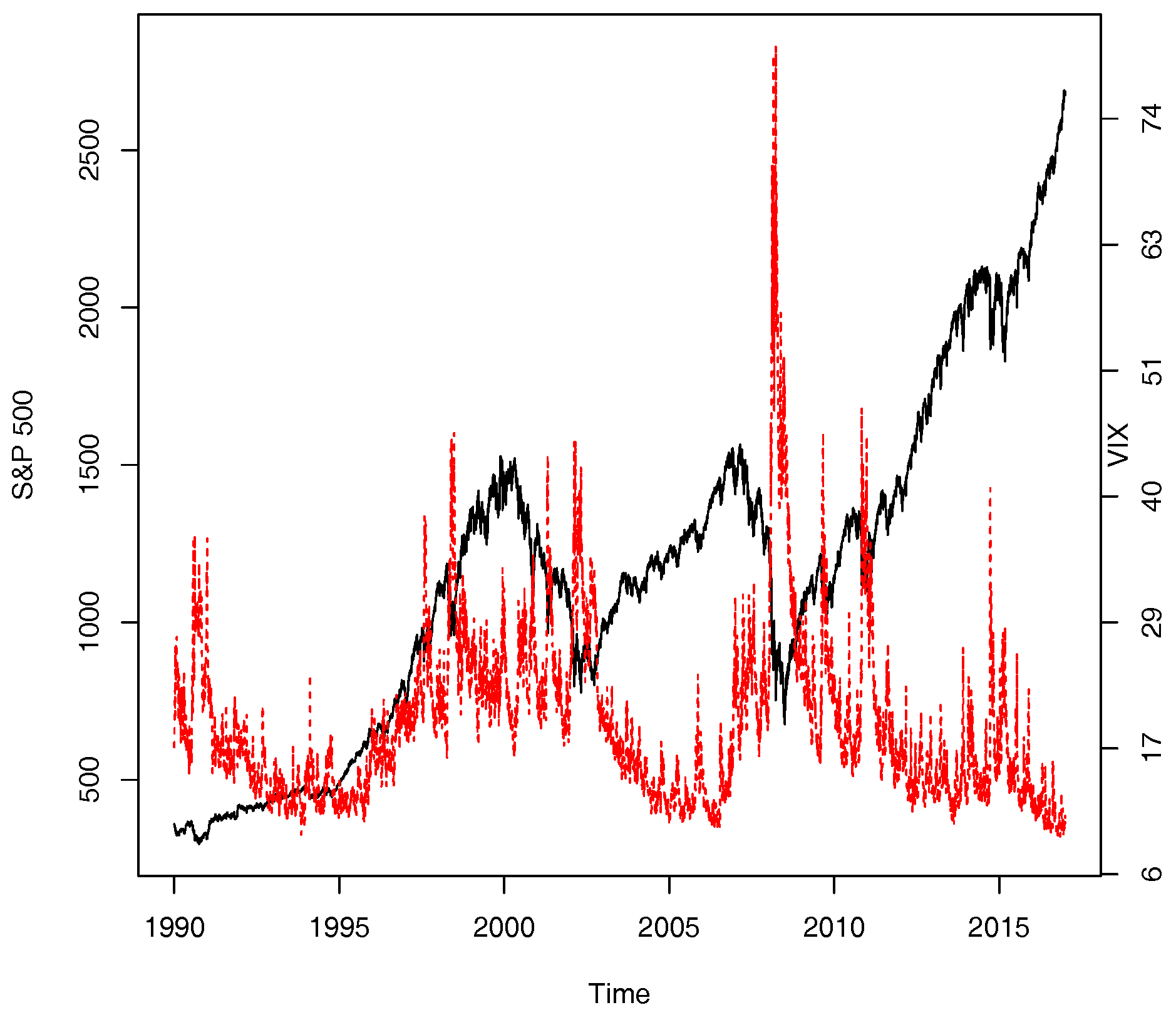
Investors witnessed severe downturn in the U.S. stock market in the second half of the year 2008 when the mood of the bearish market was often cited through an implied volatility index—the VIX, a trade mark held by the Chicago Board Options Exchange (CBOE). The VIX is designed to retrieve the market’s estimate of average S&P 500 index volatility over the subsequent 22 trading days. As bearish markets frequently observed counter-movements between S&P 500 index prices and the VIX, the VIX earned itself a reputation of market barometer of investors’ fear (see
Figure 1).
1 Motivated by this observation, we join the traditional finance literature to study the leverage and volatility feedback effects via the nonparametric method, where the asymmetric GARCH-in-mean type of models are popularly used in such a study (see
Bekaert and Wu (
2000), and references therein).
To explain a stylized fact of stock markets—the asymmetric volatility: Volatility responds more to a drop in the value of a stock (index) than an increase of an equal amount in the value of the stock (index); two popular hypotheses have been put forward such as the leverage and volatility feedback effects hypotheses; see
Black (
1976);
Bollerslev and Zhou (
2006);
Campbell and Hentschel (
1992);
Christie (
1982);
French et al. (
1987), among many others. From the empirical financial econometrics point of view, the two hypotheses explain opposite causality between stock price movements and volatility. So, which direction of causality is stronger? The answer is inconclusive; see,
Bekaert and Wu (
2000);
Bollerslev et al. (
2006), among others. Moreover, there is no agreement on which data set shall be used. For example, the literature has seen volatility measured by historical volatility, conditional volatility, realized volatility and implied volatility. A noticeable research study has been made to learn the information content of the four different volatility measures; for example,
Christensen and Prabhala (
1998);
Fleming (
1998);
Blair et al. (
2001);
Poon and Granger (
2003);
Becker et al. (
2009);
Jiang and Tian (
2005), among many others.
In this paper, we use the VIX as the measure of volatility. The VIX is published by the CBOE almost continuously each trading day such that it is public information available to all investors. Therefore, it will be a public interest to learn more about how the two publicly observable series, the S&P 500 index and its implied volatility index (or VIX), interact with each other. In addition, in empirical finance literature, the relationships between VIX (or the VIX changes) and market returns are popularly studied in semiparametric or parametric regression framework, which can potentially suffer model misspecification problem. For example,
Bollerslev and Zhou (
2006) and
Bekiros et al. (
2017) estimate the leverage and volatility feedback effects from several competitive parametric models and notice that the magnitude of these effects is very sensitive to the underlying model used for the analysis. In this paper, we therefore introduce a model-free approach to reinvestigate the causality between the implied variance (or the changes in VIX) and the market returns, by estimating the joint density functions of the two variables of interest. Specifically, we apply the nonparametric copula technique developed by
Wu (
2010) to estimate the joint density functions.
The current paper contributes to the existing literature in two folds: a new methodology and new empirical findings. In the aspect of a new methodology in studying the leverage and volatility feedback effects, we attach both effects to market specific conditions by proposing a nonparametric conditional dependence index (see
Section 4). Take the leverage effect as an example. It is a common practice in the traditional finance literature that volatility asymmetry is linked to the sign of market returns (or the sign of market return innovations) in asymmetric GARCH-type models, where a negative leverage parameter is seen as an evidence supporting the leverage hypothesis. Our proposed method, however, can be used to uncover the strength of the leverage effects across different market conditions, as we directly measure the dependence of the implied variances on S&P 500 index returns given that S&P 500 returns fall into different segments of the return distribution. Consequently, our results enable investors to understand under what circumstances they should pay particular attention to the leverage effect of the market returns on the market expected future volatility. Here, the concept of the
leverage effect is extended to the impact of the (contemporaneous and lagged) S&P 500 index returns on the implied variances.
One advantage of our research is that we attach the leverage effect with the performance of S&P 500 index, while traditional research, using asymmetric GARCH-type models to study the leverage effect, tends to define the leverage effect with respect to a predetermined reference point, usually zero.
2 Interestingly, we find that the leverage effects exhibit a W shape across different segments of S&P 500 index return distribution. To our knowledge, this is an interesting new finding that has not been documented in the finance literature: When studying the leverage effects of market returns, one needs to look beyond how market volatility reacts to positive or negative market returns.
The volatility feedback effect documented states that market returns are positively correlated with market volatility, and the returns are high (low) if the anticipated volatility increases (decreases). GARCH-in-mean type of models are usually used to test the volatility feedback effect (e.g.,
Poterba and Summers (
1986);
French et al. (
1987);
Campbell and Hentschel (
1992);
Glosten et al. (
1993)), where the coefficient for volatility effect is assumed to be a positive constant.
Bekaert and Wu (
2000) did allow market volatility to bear a varying risk premium when modeling excess stock (index) returns of Japanese market by assuming a conditional version of the CAPM based on the riskless debt model; however, the volatility feedback effect is difficult to be estimated accurately as stated in their paper. In this paper, the conditional dependence index proposed in
Section 4 is a model-free measure of the volatility feedback effect. We find that the volatility feedback effect is a U-shape curve as the squared VIX moves across different segment of its distribution. In contrast to
Bekaert and Wu’s (
2000) finding, but consistent with
Engle and Ng (
1993) and references in
Bollerslev et al. (
2006), we find that the volatility feedback effect is generally smaller than the leverage effect.
Most researchers agree that the implied variance, VIX, has a long-memory of its past, while S&P 500 market returns have a very short memory of its past. We therefore decompose the logarithm of the implied variance into two components: its previous day value and its daily increment (named in this paper). We show that the log-increment of the VIX has very short memory comparable with the market return. Since the relation between market returns and the implied variance is a balanced or net outcome of the relation of the market returns with each component of the implied variance, we then explore the instantaneous relation between the short-memory component of the implied variance and the market returns. That is, we investigate not only the leverage and volatility feedback effects along the line of the traditional finance literature, but also study the relation between the log-increments of the VIX and the market returns. Our empirical findings are consistent with our intuition: we observe considerable contemporaneous dependence between S&P 500 index returns and the logarithm changes of the VIX, which is bigger than both the leverage and volatility feedback effects in terms of magnitude in general.
The strong daily, negative, asymmetric relation between the market returns and the increments of the market volatility is also found in
Giot (
2005) and
Hibbert et al. (
2008) in a simple linear regression model framework and
Bekiros et al. (
2017) in a linear quantile regression setup. Our analysis provides several additional noteworthy results: (a) the two series exhibit strong, negative, extreme tail dependency; (b) the negative dependency is stronger in extreme downturn markets than in extreme bullish markets; (c) the dependency gradually weakens as the market return moves toward the center of its distribution, or in quiet markets. These results imply that the simple linear regression model with a dummy variable to account for positive or negative market returns may not be sufficient to capture the extreme tail relation between the log-increments of the VIX and the S&P 500 index returns and that the average relation implied by the linear regression model may understate the relation of the two series in extreme market conditions.
The rest of the paper is organized as follows.
Section 2 presents the data and summary statistics.
Section 3 discusses the nonparametric estimation of copula joint densities and presents the tail dependence indexes of interest. In
Section 4, we propose a conditional dependence index to study the leverage and volatility feedback effects and the relation between market returns and the log-increments of the VIX. To check on the robustness of the results, we conduct subsample analysis by splitting the data into four subsample periods. We conclude in
Section 5.
2. Data and Descriptive Statistics
We downloaded daily S&P 500 index prices from DataStream and daily implied volatility (or VIX) from the CBOE. The data span from 2 January 1990 (the first date that the VIX is available) to 29 December 2017. The VIX is designed to provide a benchmark market volatility index measuring the market’s aggregate view of the average market volatility over the subsequent 22 trading days, calculated from both at-the-money and out-of-the-money S&P 500 option contracts satisfying some volume conditions (
Whaley 1993,
2000) via a model-free method developed by
Demeterfi et al. (
1999) and originated from the seminal work of
Breeden and Litzenherger (
1978). Detailed information about the VIX can be found at
http://www.cboe.com.
The VIX is frequently cited as a barometer of investors’ fear, and this view of the implied volatility has found strong popularity among the investor community. A high VIX beyond 40 is usually linked to a severe bear market while a low VIX value to a market with more confidence. The first time that the VIX surpassed the value of 40 was on 31 August 1998, a year marked by Russia’s currency devaluation and national debt moratorium and the collapse of the Long Term Capital Management in the U.S.A. The number of transaction days with the VIX value exceeding 40 is 15, 4, 10, 63, 61, 3, 11, and 1 in the year of 1998, 2001, 2002, 2008, 2009, 2010, 2011, and 2015, respectively. On 20 November 2008, the VIX reached its record high of 80.86, marking an unprecedented financial crisis faced by global financial markets.
We plot the two data series in
Figure 1. For the data period under consideration, the two indexes moved in opposite directions in 77.68 percent of the total transaction days. Splitting the data according to the directions of the S&P 500 index price movements, we observe this: of 77.08 percent of the total 3285 transaction days that the S&P 500 index fell, the VIX gained; of 78.30 percent of the total 3765 transaction days that the S&P 500 index gained, the VIX fell. We also see a significant increase in counter-movements between the two indexes during extremely bearish market periods; for example, the two series move in opposite directions 84.92%, 88.93%, and 80.15% of the transaction days in the year of 1998, 2008, and 2009, respectively.
Let
and
be the S&P 500 index price and the
implied variance at date
t, respectively.
3 We construct the daily S&P 500 index return and the log-increment of the VIX as follows:
Table 1 reports the summary statistics of the implied variance, S&P 500 index returns, and log-changes of the VIX. It is noted that
has a slightly lower average but significantly higher variation than
during the sample period. We then split the data according to the sign of
and calculate the upside and downside averages and sample standard deviations for both
and
. Interestingly, we observe that both series exhibit stronger volatility in the downturn markets than in the upturn markets. In the downturn markets, the market index performed considerably worse than in the upturn markets, and the opposite holds true for the VIX index. In addition, the implied variance,
, is on average lower and less volatile when the S&P 500 index prices went up than when the S&P 500 index prices came down.
4 Next, we use three dependence measures between
and
to examine the counter-movements between the S&P 500 index prices and the VIX values, including Pearson’s correlation coefficient, Kendall’s tau,
5 and
. Kendall’s tau reveals a strong negative (or positive) association between the two series if it is close to negative (or positive) one, and a weak association if it is close to zero. Kendall’s tau equals zero, if the two series are independent, but it may not hold true vice versa. As for
, the probability that the two series move in opposite directions, the closer
is to one, the stronger is the negative association between
and
. We report our estimates in the fourth to sixth columns in
Table 2. The sample correlation between
and
ranges from −0.878 in 2015 to −0.450 in 1995 and Kendall’s tau ranges from −0.727 in 2015 to −0.295 in 1995. The negative dependence was more prominent in the past 18 years of the 21th century than in the 1990s. For the entire sample period under consideration, there is a 77.7 percent chance that the S&P 500 index prices and the VIX values moved in opposite directions, and this number peaked at 88.9 percent in 2008 and bottomed at 63.9 percent in 1995. Roughly speaking, the worse the market is, the stronger is the negative dependence.
The second and third columns of
Table 2 report the sample correlation and Kendall’s tau of (
), which give an overall measure of the relation between the expected near future market aggregate risk and current market aggregate return. All these statistics are negative and significantly different from zero at the 5% level, but less prominent than those between
and
. The overall lower negative relation between
and
is not a surprise, given the fact that the
is a long-memory process while the
has a very short serial correlation with itself; see
Table 1.
To sum up,
Table 2 indicates a significant negative relation between the market returns and the log-increments of the VIX (and market implied variance). At the same time, we also notice that the negative relation is stronger when the market index performs poorly than when the market index performs well. It implies that an overall negative association between the two series cannot tell the full story of how the two series relate. This observation motivates us to examine the joint distribution of the two series in the next section.
3. Copula Function and Tail-Dependence Index
To further our understanding of the dependence relationship between the S&P 500 returns and the log-increments of the VIX and between the S&P 500 returns and the
, we use the device of copula to decompose their joint probability density functions (or p.d.f.’s). According to the Skalar’s theorem, the joint density of two continuous random variables
X and
Y can be written as
where
X has a marginal p.d.f.
and a cumulative distribution function (or c.d.f., hereafter)
, and
Y has a marginal p.d.f.
and a c.d.f.
. As a function of the c.d.f.’s of
X and
Y, the
copula density function,
, captures completely the dependence structure between
X and
Y. We refer interested readers to
Nelsen (
1999) for a thorough treatment of the copula method and
Cherubino et al. (
2004) for applications in finance.
As a powerful tool to measure extreme co-movement across different international stock markets and different assets, copulas have been widely used in empirical finance literature to explore nonlinear tail dependence; e.g.,
Chollete et al. (
2011);
Liu et al. (
2017) and references therein. However, it is common practice for researchers to assume a certain parametric copula function in their analysis, which can create a model misspecification problem. The commonly used parametric copula families (e.g., Gaussian copula, Student’s t copula, and Fréchet copula) implicitly impose a specific dependence structure between
X and
Y, which may not be supported by empirical data. For example, Gaussian copula density assumes that the two variables have a constant correlation regardless of whether
X and
Y are around the median or tails of their respective distributions. This dependence structure imposed by Gaussian copula evidently is not consistent with the fact documented in the preceding section that the dependence between the S&P 500 index returns and the implied variance is stronger during severe bearish market periods, which is featured with unusually high implied variance and low S&P 500 index returns, than during quiet market periods with relatively low implied variance. Therefore, in this paper, to avoid misspecifying the dependence structure of
and of
, we shall adopt a nonparametric copula method proposed by
Wu (
2010) to estimate their copula density functions. Allowing the data to speak out their true relation,
Wu (
2010) proposes an exponential series copula density estimator (henceforth, ESE) without preassuming the parametric form of dependence structure between two series of interest.
Below, we briefly explain the ESE estimator, denoting
and
to simplify our notation. Firstly, to guarantee a positive copula density function, we approximate it by
where
m is a positive integer, and
is a constant to ensure that
integrates to unity. The ESE can be viewed as a series approximation of the log density, and the functional form of
is determined by
m, which is the order of polynomials of the log copula density.
Secondly, to estimate the parameters,
, in (
3), we apply
Jaynes’ (
1957) famous Maximum Entropy (ME) Principle, which minimizes Shannon’s information entropy
subject to the following integration-to-unity condition and
m moment conditions
Finally, in practice, letting the number of moments increase with sample size at an appropriate rate and replacing the population moments in (6) with their corresponding sample moments, one obtains a consistent nonparametric estimator of the underlying copula density function. The sample moments are sufficient statistics of the underlying distribution, and the MLE estimator of the ME density can be shown to be asymptotically efficient (
Crain 1974).
Jaynes’ (
1957) ME Principle suggests that one can use a number of sufficient statistics that depict the copula density function. For example, if
X and
Y are drawn from a bivariate normal distribution, it is well-known that knowing the mean and variance suffice to identify the Gaussian copula density function; i.e.,
m will be two. As one does not know the true copula density function in practice, an incorrectly selected set of sufficient statistics would lead to misleading inference on the dependence relation between variables of interest. How does the choice of the set of sufficient statistics affect our estimation of the copula density function? The intuition is this: a smaller set of sufficient statistics may omit important, relevant information associated with some missing sufficient statistics, which will evidently lead to biased inference on the true dependence structure between the two variables of interest; on the other hand, a larger than necessary set of sufficient statistics will incorporate redundant information associated with the inclusion of some non-useful extra moments, inflating the variation in the estimation of
’s because of the loss of degree of freedoms. Therefore, the set of sufficient statistics, or more precisely, the order of
m of polynomial in the exponent of Equation (
3) shall be selected carefully. In fact, one can view
m as a
smoothing parameter in the framework of nonparametric density estimation. In this paper,
m is selected in a data-driven manner according to the Akaike Information Criterion (AIC), an information criterion balances the trade off between accuracy and complexity in model construction.
6 Now, let the marginal cumulative distribution functions of
,
and
denoted by
,
, and
, respectively.
7 Since these quantities are usually unknown, we replace them by their frequency estimates, i.e.,
,
, and
, respectively. Several benefits could result from the one-to-one transformation of the variable of interest via its cumulative distribution function: (a) it can effectively mitigate potential outlier problems in the nonparametric estimation; (b) as a measure of the likelihood of the occurrence of an event, probability provides a more direct way of capturing market relative status than the raw data value does across time, which is of the upmost important in our study of the relationship between the two indexes in a quick-changing market environment. Furthermore, the study of the transformed data
and
, instead of the raw data, provides a key tool to consolidate historical study of similar situations so that we can discuss the relation between two series according to event probabilities. This point will be illustrated in the next section where we discuss the full sample and subsample results.
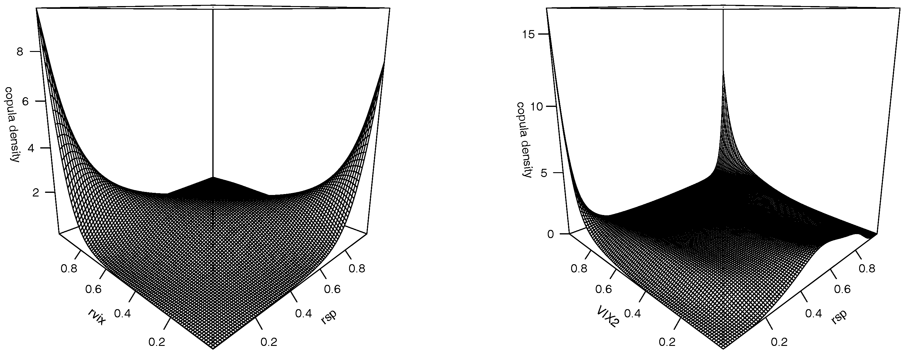
In
Figure 2, we plot the estimated copula density functions for
with
and for
with
, where
m’s are selected to minimize the AIC. The preliminary results in
Section 2 indicate a strong negative association between
and
without identifying the sources of the observed relation. The left panel in
Figure 2 suggests that the negative dependence between the S&P 500 index returns and the log-increments of the VIX is largely driven by the counter-movements at the two tails, since the bulk of the copula density is along the anti-diagonal line and spikes up at the two corners. In other words, the co-movements of the opposite tails of the two marginal distributions contribute significantly to the negative dependence between the S&P 500 index returns and the log-increments of the VIX. In addition, the density at the upper left corner in this graph, corresponding to the case of low market index returns and high VIX changes, is larger than its counterpart associated with high market index returns and low VIX changes. Except for the two tails along the anti-diagonal line in the
unit square, the copula density appears to be rather symmetric.
The right panel in
Figure 2 plots the estimated copula density for
, where we observe that the S&P 500 index returns and the
are strongly dependent when the implied variance is extremely high or its c.d.f. is close to one. The dependence is stronger when the market returns are extremely low and the implied variance is very high than when both the market returns and implied variance are extremely high. Or, put in other words, the estimated copula density indicates that the S&P 500 index returns and the
is highly dependent during high volatile markets and the dependency is stronger in a panic triggered high volatile market than an exhilarated high volatile market. On the other hand, we observed that the dependence between the two variables flattens out when the implied variance locates between its 10th percentile to its 80th percentile. We also note that the estimated copula density humps up a bit when the implied variance locates to its left tail.
To sum up, the two joint copula densities consistently show that in a low volatility market environment, which usually accompanies limited movements in the changes of the VIX level, the dependencies between S&P 500 index returns and implied variance and between the market returns and log-increments of the VIX is less noticeable.
3.1. Tail Dependence Index Between and
The joint copula density of
in
Figure 2 clearly exhibits the left-right and right-left tail dependence between the S&P 500 index returns and log-increments of the VIX. To quantify the prominent tail dependence between the two series, one naturally wants to investigate the probability with which
lies to the lower or upper tail area when
resides in the opposite tail area.
8 As the dependence occurs at the tails, such probability is usually called
tail dependence index (or TDI, henceforth). This idea is not new and has been studied in different fields. For example,
Poon et al. (
2004) studied one particular tail index using extreme value theory, although they focus on the limited cases; that is, TDI
when
or
, where
and
are the
th percentile of
X and
Y, respectively. Taking clues from the estimated copula density seen in the left panel of
Figure 2, we focus on the following two TDIs that capture the co-movements of opposite tails of
:
where
and
are the
th percentile of the return series
and
, respectively.
Taking
and
respectively, we obtain
,
,
, and
from the estimated copula density exhibited in
Figure 2. If the two series were independent, we would obtain
for
. Therefore, the fact that
is substantially higher than
indicates strong negative tail dependence between
and
series. In particular, our results suggest that extreme movements in the S&P 500 index are associated with extreme movements of the VIX to the opposite direction with high probabilities.
In addition, the fact that for both and reveals that the VIX asymmetrically responds to extreme movement of the S&P 500 index prices. The probability that the VIX increases abruptly when the market index faces free-fall is much higher than the probability that the VIX falls back when the market index price enjoys strong rebound. The asymmetry is consistent with the stylized fact frequently documented in the finance literature that the market tends to respond more to bad news than to good news of equal magnitude, although this stylized fact is described from our point view of tail dependence indexes.
The fact that the tail dependence is more pronounced when the market is in turmoil explains why the VIX is dubbed as the Investor Fear Gauge.
3.2. Tail Dependence Index Between and
As the right panel of
Figure 2 exhibits a prominent dependence between the S&P 500 index returns and implied variances when the latter reside at the right tail of its distribution, we introduce the following four TDIs:
where
is the
th percentile of the
series. We use
to illustrate the meaning of each index. First,
and
measure the probabilities that the S&P 500 returns reside to the respective right and left 1% tail of the return distribution in an extremely volatile market condition. Second,
and
give the probabilities that the market sees extremely high volatility with the implied variance falling to its upper 1% tail of its distribution in an extremely high and low market return periods.
By construction, and reflect the volatility feedback effect of market volatility on market returns at extreme situation, while and reflect the leverage effect of market returns on market volatility at extreme situations. Of course, the leverage and volatility feedback effects referred to here are extended from the traditional meaning of the two effects.
Again, we take
and
. From the estimated copula density function shown in
Figure 2, we calculate
,
,
,
,
,
,
, and
. As
for all the cases studied, we see apparent tail dependence between the market returns and market implied variances, although the tail dependence of the implied variances on the market returns is generally weaker than that of the changes of VIX on the market returns. In addition,
and
for both
and
, indicating asymmetric tail dependence between the market returns and implied variances; i.e., the TDIs are stronger when the market returns lie to the left tail of rather than to the right tail of the return distribution.
3.3. Contemporaneous and Lagged Conditional Distributions
The tail dependence index only describes the probability of the occurrence of one rare event given that of another rare event. In this section, we aim to extract more information from the data by estimating the conditional cumulative distribution (or c.c.d.f., henceforth) functions via the nonparametric copula method. Specifically, let
A be a subset of
. We are interested in estimating the conditional c.d.f.’s listed in
Table 3.
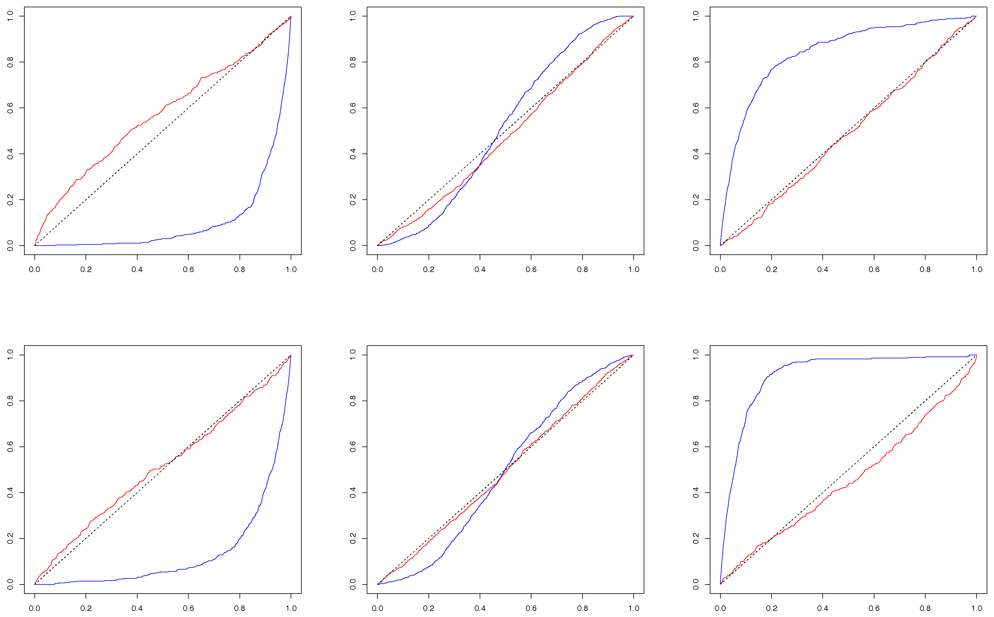
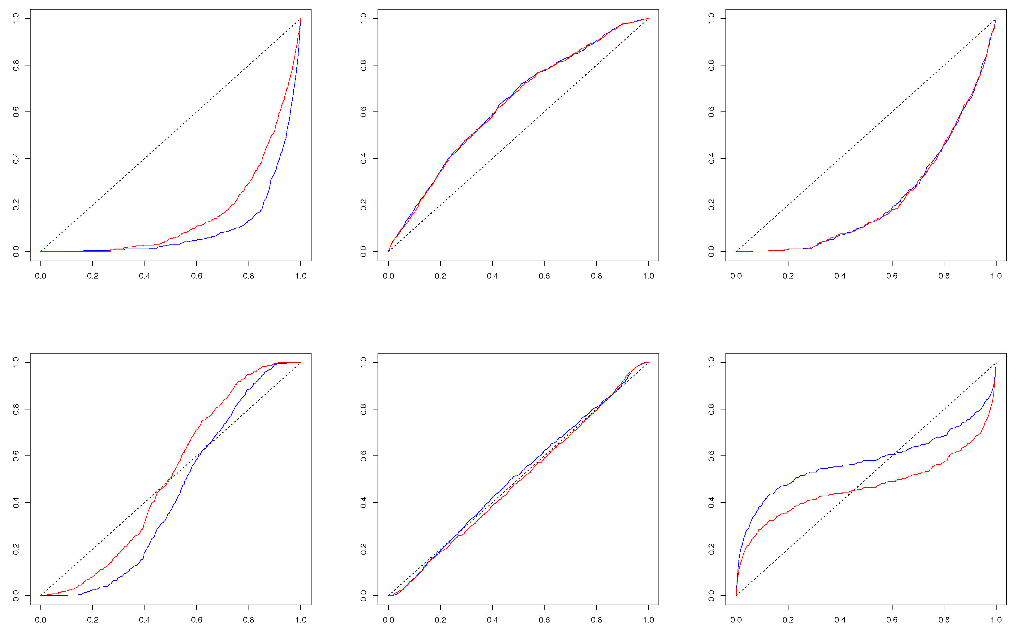
Figure 3 plots the estimated conditional c.d.f.’s for cases C1 and C2, while
Figure 4 for cases C3 and C4, wherein the results for
and
are in color blue and red respectively. Taking
,
, and
, we aim to study the behavior of the conditional c.d.f.’s under extreme and moderate market conditions. If each pair of variables among
v,
and
were drawn from a bivariate normal distribution, one would expect the conditional c.d.f. invariant with respect to the choice of
A. In addition, the choice of
or 1 is used to measure the strength of contemporaneous relation relative to lag-one relation. Examining
Figure 3 and
Figure 4, we aim to visually test two hypotheses summarized in
Table 4.
Reading
Figure 3, we observe that both the hypotheses H
and H
fail to hold for all the contemporaneous c.c.d.f.’s. Evident deviations of the c.c.d.f.’s from the 45-degree line result from strong tail dependence between the log-increments of the VIX and the market returns. On the other hand, the inter-dependence between the two series are rather mild during quiet market periods. Evidently, the results in
Figure 3 support the varying dependence relation between the two series across different market conditions, which suggests the inadequacy of fitting the data with bivariate normal distribution with a constant correlation. When
, the hypothesis H
holds roughly true for all the lag-one conditional c.d.f.’s (or l.c.c.d.f.’s, hereafter), as they are all close to the 45-degree line. Combining our observations, we see strong daily contemporaneous dependence between the market returns and log-increments of the VIX and very weak if nothing at all one-day lag dependence. Actually, when we push
h up to 20, we did not see significant lag dependences between the two series.
Let us next look at
Figure 4. Different from
Figure 3, the c.c.d.f.’s and l.c.c.d.f.’s are very close to each other, which is especially true for the conditional c.d.f.’s of
given
(in the first row of
Figure 4), implying a strong persistent dependence of the implied variance (
) on the current and one-day lagged S&P 500 index returns. Again, as in
Figure 3,
Figure 4 rejects the hypothesis H
for all the cases. The hypothesis H
seems to hold only for the c.c.d.f.’s and l.c.c.d.f.’s of
given
. Overall, the c.c.d.f.’s and l.c.c.d.f.’s of
given
deviate from the 45-degree line more than those of
given
.
To sum up, we observe strong contemporaneous left-right and right-left tail dependence between and , significant contemporaneous and lagged tail dependence of the VIX on the market returns, and mild tail dependence of the market returns on the VIX. Although useful, these qualitative assessments are largely based on smoothing and visualization of data. In the next section, we propose a conditional dependence index to formally quantify the conditional dependence between each pair of series of interest among the market returns, the log-increments of the VIX, and the VIX.
4. Conditional Dependence Index
As we discuss above,
Figure 3 and
Figure 4 plot several estimated conditional distribution functions of
u given
, where
A is a nonempty subinterval of the interval
. If
u and
v are independent of each other when
, we have
for all
so that knowing the information
does not help us make better predictions about
u. On the other hand, the further is the conditional c.d.f. away from the 45-degree line, the higher is the dependency between
u and
. Therefore, it is natural to use the area between the conditional c.d.f. and the 45-degree line as a proxy of the predictive power of
on
u. In doing so, we are able to learn under what circumstances
u and
v are most dependent as
v moves across its distribution function. Consequently, we can make inference on the relation between the pair of variables of interest conditional across different market status.
Hence, we propose a conditional dependence index (or CDI, henceforth) which equals twice of the area between a conditional c.d.f. and the 45-degree line, given the fact of
. Thus, the index is defined as a functional of
A:
Evidently, for any given sub-interval
,
, where
means independence between
u and
v given
, and the dependence of
u on
grows as
gets closer to the unity. Partitioning the
interval into 20 equal-width intervals, we calculate
for each interval and report the results in
Table 5 for both
and
.
Now, we illustrate the estimation method and the test for
for the case that
, the CDI of the log-increments of the VIX on the market returns. (The method is also applied to the other cases). We denote the estimator of
by
, which is given by
where we replace the unknown conditional c.d.f.
by its empirical conditional distribution,
with the total sample size,
n = 7055,
being the indicator function, and
and
being the unconditional c.d.f.’s of
and
, respectively.
is a consistent estimator of as and the sample mean is a consistent estimator of a population mean, given the fact that both series are stationary. Actually, .
Next, we are interested in testing the null hypothesis of against the alternative hypothesis of . If the null hypothesis holds true, we can show that converges to a normal random variable with zero mean and finite variance. Under the alternative hypothesis, we expect . Therefore, we expect under the null hypothesis and under the alternative hypothesis. However, to conduct the test, we need to obtain proper critical values. As the distribution of under the null hypothesis does not have a simple formula, we propose to use bootstrap critical values.
Bootstrap critical values. Should the alternative hypothesis hold true, the realization of the log-increment of the VIX is affected by the realization of the market return. Therefore, the temporal ordering of the market return matters in the calculation of
. However, should the null hypothesis hold true, we have
, the empirical c.d.f. of
, which does not depend on the realization of the market returns, nor does
. Therefore, the temporal ordering of the market returns should not matter in the calculation of
, should the null hypothesis hold true. Based on these observations, we propose to obtain bootstrap samples by randomly shuffling the market returns while keeping the order of the log-increments of the VIX. As a result, the bootstrap sample contains the raw data on
and the randomly shuffled market return data,
, and the bootstrap sample size is the same as the original sample size, n = 7055. To obtain the bootstrap critical value at the significance level of 5% for example, we repeat 500 bootstrap procedures and use the 95th percentile of the 500 bootstrap statistics,
, to approximate the critical value, where
is the bootstrap estimate of
using (
15).
In
Table 5, we report
for six cases: the CDIs of
given
,
given
,
given
for
(capturing contemporaneous dependence) and for
(capturing one day lagged dependence).
9 We divide the interval
into 20 intervals with equal increments of 0.05. In
Table 5, we marked the insignificant CDI estimates at the 5% level with an asterisk. The fifth column of
Table 5 indicates little dependence of the log-increments of the VIX on the previous day’s market index performance. Combining the second and fifth columns, we see close contemporaneous but less noticeable lagged relation between the changes of the VIX and the market returns. In contrast, the relation between implied variance and market returns are rather persistent but become weaker in general over time, where the persistent relation may result from the long-memory properties of the implied variance.
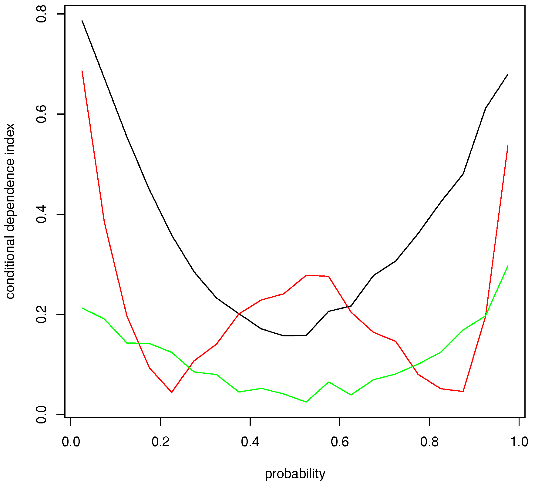
To enhance the readability of the results given in
Table 5, we plot the contemporaneous CDIs in
Figure 5. The black line shows how the distribution of the log-increments of the VIX depends on the market return as the market return moves from its lower 5% tail, (0.05, 0.10], (0.10, 0.15,], ..., to its upper 5% tail, where each probability interval contains equally 5% of the data. It shows a general U-shape curve, bottoming at the interval of (0.45, 0.50]—around the median of the market returns. The dependence of the distribution of the log-increments of the VIX on the market returns grows as market returns go farther away from its median, although the dependences grow faster with steeper slope when the market return falls below its median value than when the market return grows above its median value (for the full sample, the daily market average return is 0.04584%). At the extreme market cases, the CDI of the log-increments of the VIX takes the highest value .787 when the market return falls below its lower 5% tail, which is higher than .680 when the market return grows beyond its upper 5% tail. The finding reflects the market’s asymmetric attitude toward an extreme down market and an extreme upper market: investors in general feel more nervous in the former than the latter situation.
Below, we will link our empirical results found in this section to the traditional findings on the leverage and volatility feedback effects. Here, we refer to the leverage effect as the dependence of the implied variance on the market returns at lag one and the volatility feedback effect as the dependence of the market returns on the implied variance at lag one.
The leverage effect. The red line in
Figure 5 shows how the distribution of the
depends on
as the market returns move from the lower 5% tail to the upper 5% tail of the return distribution. Surprisingly, we observe that the CDIs exhibit a W shape. The leverage effect is strongest when the market return falls below its 5% lower tail. If we call the volatility resulting from the market’s expectation of a bright and a dismal future as good volatility and bad volatility, respectively, our results indicate that the dependence of the good volatility on market return is evidently lower than that of the bad volatility. This is consistent with the “asymmetric volatility” phenomenon documented in the literature (e.g.,
Aboura and Wagner 2016). We also observe strong leverage effect over the probability intervals, [0.4, 0.45), [0.45, 0.5), [0.5, 0.55), and [0.55, 0.6), and the noteworthy leverage effect when the market return falls into its [0.5, 0.55] probability interval dominates the relation of the log-increments of the VIX on the market return in the same probability interval. As the middle segment of the market return distribution symbolizes a very quiet market state; during which period, the market participants have the most uncertainty over the prediction of the direction of future market returns. Our conjecture is this: The uncertainty over future market direction may cause variance premium to dominate the conditional variance of market returns as the latter can be relatively accurately estimated during quiet market periods, where the implied variance equals the sum of variance premium and the conditional variance of market returns as defined in
Bekaert and Hoerova (
2014) who found that the variance premium is a component of the implied variance to predict future market returns.
The volatility feedback effect. The green line in
Figure 5 shows how the distribution of
depends on
, where we see a much flatter convex curve than the black curve. The right most column of
Table 5 shows that the volatility feedback effects are insignificant at the 5% significance level when the market return falls into the probability interval of [0.3, 0.35) to [0.6, 0.65). This means that we would not find a noticeable volatility feedback effect if we fit the data with a mean regression model. This result may be used to explain why empirical works cannot find volatility feedback effects with GARCH-in-mean model; e.g.,
Campbell and Hentschel (
1992).
Comparing the three curves, we find noticeably higher dependence between the market returns and log-increments of the VIX than the leverage and volatility feedback effects, except for a higher leverage effect when the market return is moving around its medium value. This result encourages the econometric modeling of the market returns and log-changes of the VIX besides the leverage and volatility feedback effects. In addition, the volatility feedback effect is weaker than the leverage effect with some exceptions. This result may support the findings in
Christie (
1982) and
Bekaert and Wu (
2000) that neither the leverage effect nor the volatility feedback effect can be the sole explanation of the volatility asymmetry observed from stock markets.
To sum up, we find strong dependence between and and the dependence is stronger in volatile market periods than in relatively quiet market periods. As the VIX reveals market’s expectation on the future 30-day volatility, our results indicate that investors make sharp revision on their belief of market risks during extreme volatile market periods, and that the revision is less noticeable during tranquil market periods. This again confirms that the negative association between the S&P 500 index prices and the VIX mainly come from tail events.
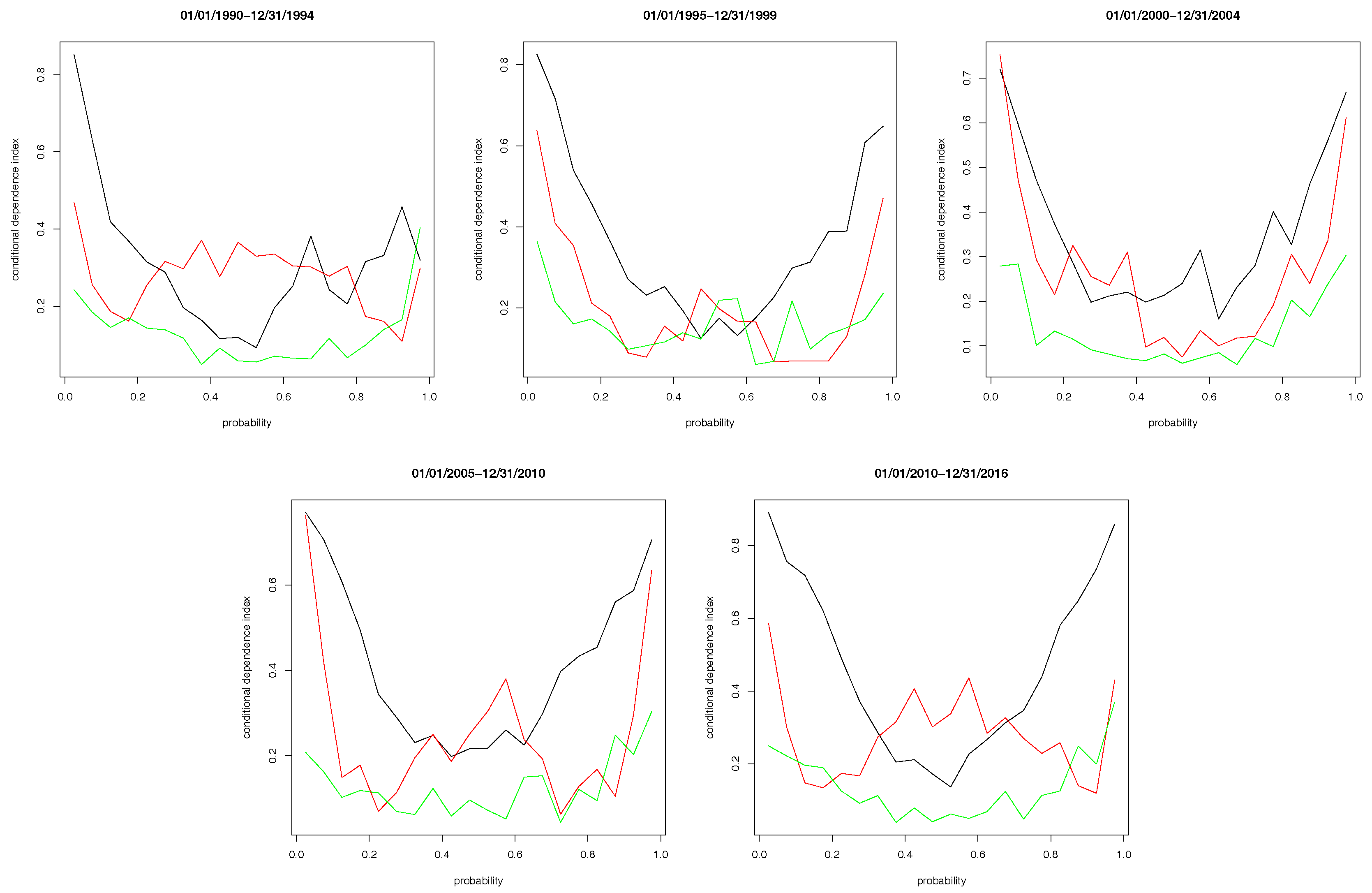
To check on how robust our findings are, we also conduct subsample analysis, where we split the sample period into five subperiods: 2 January 1990 to 31 December 1994; 1 January 1995 to 31 December 1999; 1 January 2000 to 31 December 2004; 1 January 2005 to 31 December 2009; 1 January 2010 to 31 December 2017.
10 Figure 6 plots the estimated CDIs for the four subsample periods. In general, the subsample results are similar to the full sample results shown in
Figure 5, except for the first subperiod.


