Negative Binomial Kumaraswamy-G Cure Rate Regression Model

Abstract

In survival analysis, the presence of elements not susceptible to the event of interest is very common. These elements lead to what is called a fraction cure, cure rate, or even long-term survivors. In this paper, we propose a unified approach using the negative binomial distribution for modeling cure rates under the Kumaraswamy family of distributions. The estimation is made by maximum likelihood. We checked the maximum likelihood asymptotic properties through some simulation setups. Furthermore, we propose an estimation strategy based on the Negative Binomial Kumaraswamy-G generalized linear model. Finally, we illustrate the distributions proposed using a real data set related to health risk.

1. Introduction

In survival analysis, the study is based on data relating to the time until the occurrence of a particular event of interest, also known as time to failure. This data can come from the time until there is a failure in an electronic component; time until a particular disease occurs in a patient; time for a particular drug to have the desired effect, among others. The behavior of such data can be verified empirically; this approach is said to not be parametric. If the data follows a probability distribution, then this approach is called parametric; this is the most used form in this work.

The survival and hazard functions, the objects of greatest interest in survival analysis, allow the study of such behavior. The survival function is the probability of an individual or component surviving after a preset time and the hazard function is the instantaneous failure rate, which graphically can take various forms, such as constant, increasing, decreasing, unimodal or bathtub shaped. However, when the behavior of the hazard function is not monotonous, the most commonly known distributions, such as exponential and Weibull, cannot accommodate this kind of behavior.

This is because a disadvantage of these models is that they are very limited due to the small number of parameters and therefore the conclusions drawn from the models cannot be sufficiently robust to accommodate deviations from the data. There are some distributions that accommodate the non-monotonic hazard function, but they are usually very complicated and with many parameters.

We can model real survival data using almost any continuous distribution and with positive values; the simplest and most common models, such as exponential and Weibull distribution, may not be appropriate. Therefore, to find a distribution that accommodates non-monotone hazard functions is a known issue in survival analysis. Therefore, it is desirable to consider other approaches to achieve greater flexibility, and this is what has motivated studies to find distributions that accommodate these types of function.

Kumaraswamy (1980) proposed the Kumaraswamy distribution, which was widely used in hydrology and, based on this, Cordeiro and de Castro (2011) proposed a new family of generalized distributions, called Kumaraswamy generalized (Kum-G). It is flexible and contains distributions with unimodal and bathtub-shaped hazard functions, as shown by De Pascoa et al. (2011), and has, as special cases, any distribution that is normal, exponential, Weibull, Gamma, Gumbel and inverse Gaussian. The domain of the distribution is the range in which the particular cases are set. Other examples of generalized distributions are the Generalized exponential distribution (Gupta and Kundu 1999) and the Stoppa (or Generalized Pareto) distribution (Stoppa 1990) and (Calderín-Ojeda and Kwok 2016).

In a population, there may be individuals who have not experienced the event of interest until the end of the study; this is called censorship. When there are a large number of censored individuals, we have an indication that in this population there are individuals who are not subjected to the event; they are considered immune, cured or not susceptible to the event of interest.

From the traditional models of survival, it is not possible to estimate the cured fraction of the population, or the percentage of individuals who are considered cured. Thus, statistical models are needed to incorporate such fractions and these are termed long-term or cure rate models. Because of this capability, different fit methods have been proposed in several areas such as biomedical studies, financial, criminology, demography and industrial reliability, among others. For example, in biomedical data, an event of interest may be the death of the patient due to tumor recurrence, but there may be patients who are cured and do not die due to cancer. When the financial data is studied, an event of interest may be the customer’s closing of a bank account by default, but there may be customers who will never close their account. In criminology data, the event of interest may be a repeat offence and there may be people who do not repeat an offence. In industrial reliability, long duration models are used to verify the proportion of components that are not tested at zero time and are exposed to various voltage regimes or uses. In market research areas, individuals who will never buy a particular product are considered immune. See, for example, (Anscombe 1961; Farewell 1977; Goldman 1984; Broadhurst and Maller 1991; Meeker and Escobar 1998).

Many authors have contributed to the theory of long-term models. Boag (1949) was the pioneer; the maximum likelihood method was used to estimate the proportion of survivors in a population of 121 women with breast cancer, in an experiment that lasted 14 years. Based on Boag’s idea, Berkson and Gage (1952) proposed a mixture model in order to estimate the proportion of cured patients in a population subjected to a treatment of stomach cancer. More complex long-term models, such as Yakovlev and Tsodikov (1996), Chen et al. (1999) among others, have emerged in order to better explain the biological effects involved. More recently, Rodrigues et al. (2009) proposed a unified theory of long duration, considering different competitive causes. In this context, most long-term models make use of this proposal, among which are (Sy and Taylor 2000; Castro et al. 2009; Cancho et al. 2011; Gu et al. 2011), besides (Ibrahim et al. 2005; Cooner et al. 2007; Ortega et al. 2008, 2009; Cancho et al. 2009).

A very important point in survival analysis is the study of covariates, because many factors can influence the survival time of an individual. Therefore, incorporate covariates enable us to have a much more complete model, full of valuable information. For example, if we are interested in studying the life time of patients with a particular disease who are receiving a certain treatment, other factors may influence the patient’s healing, so we can find new ways to treat the disease from covariates. One real situation is the study of patients that were observed for recurrence after the removal of a malignant melanoma; it is desired to know if the nodule category or the age of the patient may influence the recurrence of melanoma. We will analyze this clinical study latter.

This paper presents the unified long-term model using, as a distribution of the number of competing causes, the negative binomial distribution, as studied in Cordeiro et al. (2015), where the authors use the Birnbaum–Saunders distribution of times. However, our contribution is proposing the use of a different distribution of times, i.e., the family of Kum-G distributions, which were studied only in the usual models of survival analysis, as in De Pascoa et al. (2011), De Santana et al. (2012) and Bourguignon et al. (2013). In this new model, we propose the incorporation of covariates influencing the survival time. In addition, we performed a simulation study to see how this model would behave with different sample sizes, as well as an application to a data set to demonstrate the applicability of this model.

The paper is organized as follows: in Section 2, we have the methodology, in which we present the family of Kumaraswamy generalized distributions, the unified cure rate model and a distribution used in this model, i.e., the negative binomial distribution; then, we propose a unified model Kumaraswamy-G cure rate as well as a regression approach, using the distribution Kumaraswamy exponential and its inferential methods. Section 2.7 presents some simulation studies. Application to a real data set is presented in Section 3. Finally, in Section 4, we conclude the paper with some final remarks.

2. Methodology

2.1. Kumaraswamy Family of Distributions

The time until the occurrence of some event of interest can be generally accommodated by a probability distribution. In the literature, various distributions have been used to describe survival times but most commonly used distributions do not have the flexibility to model non-monotone hazard functions, such as unimodal and bathtub-shaped hazard functions, which are very common in biological studies. Thus, in this section, we will study the Kumaraswamy generalized distribution because it is a flexible but simple distribution.

The Kumaraswamy generalized distribution (Kum-G) presented by Cordeiro and de Castro (2011) has the flexibility to accommodate different shapes for the hazard function, which can be used in a variety of problems for modeling survival data. It is a generalization of the Kumaraswamy distribution with the addition of a distribution function $G\left(t\right)$ of a family of continuous distributions.

Definition. 

Let $G\left(t\right)$ be a cumulative distribution function (cdf) of any continuous random variable. The cdf of the Kum-G distribution is given by

$$\begin{array}{c}\hfill {\displaystyle F\left(t\right)=1-{\left[1-G{\left(t\right)}^{\lambda }\right]}^{\phi },}\end{array}$$

where $\lambda >0$ and $\phi >0$. Let $g\left(t\right)=\frac{dG\left(t\right)}{dt}$ be the probability density function (pdf) of the distribution of $G\left(t\right)$, then the pdf of Kum-G is

$$\begin{array}{c}\hfill {\displaystyle f\left(t\right)=\lambda \phi g\left(t\right)G{\left(t\right)}^{\lambda -1}{\left[1-G{\left(t\right)}^{\lambda }\right]}^{\phi -1}.}\end{array}$$

Thus, we obtain the survival and hazard functions, given respectively by

$$\begin{array}{c}\hfill {\displaystyle S\left(t\right)={\left[1-G{\left(t\right)}^{\lambda }\right]}^{\phi }}\end{array}$$

and

$$\begin{array}{c}\hfill {\displaystyle h\left(t\right)=\frac{\lambda \phi g\left(t\right)G{\left(t\right)}^{\lambda -1}}{1-G{\left(t\right)}^{\lambda }}.}\end{array}$$

In the literature, there are different generalized distributions, one of which is the beta distribution. The pdf of beta generalizations uses the beta function, which is difficult to handle. On the other hand, the Kum-G distribution is a generalization that shows no complicated function in its pdf, and it is more advantageous than many generalizations.

As the Kum-G distribution depends on a $G\left(t\right)$ distribution function, for each continuous distribution, we have a case of Kum-G with the number of parameters of $G\left(t\right)$ over the two parameters $\lambda$ and $\phi$. For example, if we take the cumulative distribution function of an exponential distribution as $G\left(t\right)$, then in this case we have the Kumaraswamy exponential distribution. In the literature, many cases of this distribution were studied, some of which are Kumaraswamy normal (Correa et al. 2012), Kumaraswamy log-logistic (De Santana et al. 2012), Kumaraswamy pareto (Bourguignon et al. 2013), Kumaraswamy pareto generalized (Nadarajah and Eljabri 2013), Kumaraswamy gamma generalized (De Pascoa et al. 2011), Kumaraswamy half-normal generalized (Cordeiro et al. 2012), Kumaraswamy Weibull inverse (Shahbaz et al. 2012) and Kumaraswamy Rayleigh inverse (Hussian and A Amin 2014).

2.2. The Unified Cure Rate Model

The unified model of the cured fraction of Rodrigues et al. (2009) is a statistical model capable of estimating the proportion of a cured population, that is, in data sets in which many individuals do not experience the event of interest, even if observed over a long period of time, part of the population is cured or immune to the event of interest; we can estimate the cured fraction. Several authors have worked with this modeling, for example, (Rodrigues et al. 2009, Peng and Xu 2012; Balakrishnan and Pal 2012, 2013a, 2013b, 2015), and others.

In general, the basic idea of the unified model of the cured fraction is based on the notion of occurrence of the event of interest in a process in two stages:

Initiation stage. Let N be a random variable representing the number of causes or competitive risks of occurrence of an event of interest. The cause of the occurrence of the event is unknown, and the variable N is not observed, with probability distribution $p_n$ and its tail given respectively by $p_n=P(N=n)$ e $q_n=P(N>n)$ with $n=0,1,2,\dots$.

Maturation stage. Given that $N=n$ equal $Z_k$, $k=1,\dots ,n$, continuous random variables (non-negative), independent of a cumulative distribution function $F\left(z\right)=1-S\left(z\right)$ and independent of N, represent the time of occurrence of an event of interest because of the k-th cause.

In order to include individuals who are not susceptible to the event of interest, its time of occurrence is defined as

$$\begin{array}{c}\hfill T=min\left(Z_0,Z_1,Z_2,\dots ,Z_N\right),\end{array}$$

where $P(Z_0=\infty )=1$, admitting the possibility that a proportion $p_0$ of the population lacks the occurrence of an event of interest, T is an observable or censored random variable, and $Z_j$ and N are latent variables.

Let $\left\{a_n\right\}$ be a sequence of real numbers. $A\left(s\right)$ is defined as a function of the sequence $\left\{a_n\right\}$ as follows

$$\begin{array}{c}\hfill A\left(s\right)=a_0+a_{1}s+a_2{s}^2+\cdots ,\end{array}$$

where s belongs to the interval $[0,1]$.

The survival function of the random variable T (population survival function) will be indicated by

$$\begin{array}{ccc}\hfill S_{pop}\left(t\right)& =& P(N=0)+P(Z_1>t,Z_2>t,\dots ,Z_N>t,N\ge 1)\hfill \\ & =& P(N=0)+\sum _{n=1}^{\infty }P(N=n)P(Z_1>t,Z_2>t,\dots ,Z_N>t)\hfill \\ & =& p_0+\sum _{n=1}^{\infty }{p}_n{S\left(t\right)}^n\hfill \\ & =& A\left[S\left(t\right)\right],\hfill \end{array}$$

where $A(·)$ corresponds to a genuine generating function of the sequence $p_n$. That is, in the survival function of the random variable T, corresponding to a long-term model in two stages, the composition is a probability-generating function and survival function. The long-term survival function, in two stages $S_{pop}\left(t\right)$, is not a survival function.

Note that for the survival function, ${lim}_{t\to 0}S\left(t\right)=1$ and ${lim}_{t\to \infty }S\left(t\right)=0$. As for the improper survival function, ${lim}_{t\to 0}S\left(t\right)=1$ and ${lim}_{t\to \infty }{S}_{pop}\left(t\right)=P(N=0)=p_0$. Thus, $p_0$ is the proportion of non-event occurrences in a population of interest, that is, the cured fraction.

The population survival function has the following properties:

• If $p_0=1$, then $S_{pop}\left(t\right)=S\left(t\right)$;
• $S_{pop}\left(0\right)=1$;
• $S_{pop}\left(t\right)$ it is not increasing;
• ${lim}_{t\to \infty }{S}_{pop}\left(t\right)=p_0$.

The density and hazard functions associated with long-term survival function are given respectively by

$$\begin{array}{c}\hfill f_{pop}\left(t\right)=f\left(t\right)\frac{dA\left(s\right)}{ds}{|}_{s=S\left(t\right)}\end{array}$$

and

$$\begin{array}{c}\hfill h_{pop}\left(t\right)=\frac{f_{pop}\left(t\right)}{S_{pop}\left(t\right)}=f\left(t\right)\frac{\frac{dA\left(s\right)}{ds}{|}_{s=S\left(t\right)}}{S_{pop}\left(t\right)}.\end{array}$$

Any discrete distribution can be used to model N, such as Bernoulli, binomial, Poisson, negative binomial and Geometric. What follows is the negative binomial distribution, which will be used because it is a very flexible distribution with various special cases, including those resulting in the standard model mix.

2.3. Negative Binomial Distribution

Assuming the number of competitive causes N following a negative binomial distribution, N has the probability function defined by

$$\begin{array}{c}\hfill P(N=n)=\frac{\Gamma (n+{\eta }^{-1})}{n!\Gamma \left({\eta }^{-1}\right)}{\left(\frac{\eta \theta }{1+\eta \theta }\right)}^n{\left(1+\eta \theta \right)}^{-1/\eta },\end{array}$$

where $n=0,1,2,\dots$, $\theta >0$ e $1+\eta \theta >0$, and then $\mathrm{E}\left(N\right)=\theta$ and $Var\left(N\right)=\theta +\eta {\theta }^2$.

The probability generating function is given by

$$\begin{array}{c}\hfill A\left(s\right)=\sum _{n=0}^{\infty }{p}_n{s}^n={\left[1+\eta \theta (1-s)\right]}^{-1/\eta },0\le s\le 1.\end{array}$$

Thus, the long-term survival function for the negative binomial model is given by

$$\begin{array}{c}\hfill S_{pop}\left(t\right)={\left[1+\eta \theta F\left(t\right)\right]}^{-1/\eta },\end{array}$$

(1)

where $F\left(t\right)$ is the cumulative distribution function of the random variable T and the cured fraction of the population is

$$\begin{array}{c}\hfill p_0=\underset{t\to \infty }{lim}{S}_{pop}\left(t\right)={\left(1+\eta \theta \right)}^{-1/\eta }.\end{array}$$

The density function of the model (1) is

$$\begin{array}{c}\hfill f_{pop}\left(t\right)=-\frac{d{S}_{pop}\left(t\right)}{dt}=\theta f\left(t\right){\left[1+\eta \theta F\left(t\right)\right]}^{-1-1/\eta },\end{array}$$

where $f\left(t\right)=-S^{\prime }\left(t\right)$. Furthermore, the corresponding hazard function is given by

$$\begin{array}{c}\hfill h_{pop}\left(t\right)=\theta f\left(t\right){\left[1+\eta \theta F\left(t\right)\right]}^{-1}.\end{array}$$

We observed some particular cases in this model: from the Equation (1), when $\eta \to 0$, we obtain the density function of the Poisson distribution, resulting in the promotion time model; if $\eta =-1$, we fall into the Bernoulli distribution, where we have the model of the standard mixture; if $\eta =1$, we have the geometric distribution; when $\eta =1/m$ (m integer), we have a binomial distribution (m, $\theta /m$), where $0\le \theta /m\le 1$. We also observed, from expressions of expectation and the variance of the model, that the variance of the number of competing causes is very flexible. If $-1/\theta <\eta <0$, there is an underdispersion relative to the Poisson distribution; if $\eta >0$, there is an overdispersion.

Table 1. Survival function $S_{pop}\left(t\right)$, density function $f_{pop}\left(t\right)$, and cured fraction of different distributions of latent causes.

Distribution	${\mathit{S}}_{\mathit{pop}}\left(\mathit{t}\right)$	${\mathit{f}}_{\mathit{pop}}\left(\mathit{t}\right)$	${\mathit{p}}_0$	$\mathit{A}\left(\mathit{s}\right)$
Bernoulli$\left(\theta \right)$	$1-\theta +\theta S\left(t\right)$	$\theta f\left(t\right)$	$1-\theta$	$1-\theta +\theta s$
Binomial$(K,{\theta }^{*})$	${\left[1-{\theta }^{*}+{\theta }^{*}S\left(t\right)\right]}^K$	$K{\theta }^{*}f\left(t\right){\left[1-{\theta }^{*}+{\theta }^{*}S\left(t\right)\right]}^{K-1}$	($1-{\theta }^{*}{)}^K$	${(1-{\theta }^{*}+{\theta }^{*}s)}^K$
Poisson$\left(\theta \right)$	$exp\left[-\theta F\left(t\right)\right]$	$\theta f\left(t\right)exp\left[-\theta F\left(t\right)\right]$	$e^{-\theta }$	$exp\left[\theta (1-s)\right]$
Geometric$\left(\theta \right)$	${\left[1+\theta F\left(t\right)\right]}^{-1}$	$\theta f\left(t\right){\left[1+\theta F\left(t\right)\right]}^{-2}$	$1/(1+\theta )$	${\left[1+\theta (1-s)\right]}^{-1}$
Negative Binomial$(\eta ,\theta )$	${\left[1+\eta \theta F\left(t\right)\right]}^{-1/\eta }$	$\theta f\left(t\right){\left[1+\eta \theta F\left(t\right)\right]}^{-1-1/\eta }$	${(1+\eta \theta )}^{-1/\eta }$	${\left[1+\eta \theta (1-s)\right]}^{-1/\eta }$

presents the long-term survival function, improper density and cure rate corresponding to negative binomials and their particular cases.

2.4. Negative Binomial Kumaraswamy-G Cure Rate Model

Considering the negative binomial distribution for the number of competing causes and the time following the Kumaraswamy-G distribution, we obtain a family of long-term distributions, wherein the population survival function of the model is given by

$$\begin{array}{c}\hfill S_{pop}\left(t\right)={\left[1+\eta \theta F\left(t\right)\right]}^{-1/\eta }={\left\{1+\eta \theta \left\{1-{\left[1-G{\left(t\right)}^{\lambda }\right]}^{\phi }\right\}\right\}}^{-1/\eta },\end{array}$$

(2)

with the cured fraction of the population given by

$$\begin{array}{c}\hfill p_0={(1+\eta \theta )}^{-1/\eta }.\end{array}$$

So, by replacing the function $G\left(t\right)$ by the cumulative distribution function of some distribution, one obtains a negative binomial Kumaraswamy-G model of long-term survival.

The population density function is

$$\begin{array}{c}\hfill f_{pop}\left(t\right)=\theta \lambda \phi g\left(t\right)G{\left(t\right)}^{\lambda -1}{\left[1-G{\left(t\right)}^{\lambda }\right]}^{\phi -1}{\left\{1+\eta \theta \left\{1-{\left[1-G{\left(t\right)}^{\lambda }\right]}^{\phi }\right\}\right\}}^{-1-1/\eta }\end{array}$$

and the population hazard function is given by

$$\begin{array}{c}\hfill h_{pop}\left(t\right)=\theta \lambda \phi g\left(t\right)G{\left(t\right)}^{\lambda -1}{\left[1-G{\left(t\right)}^{\lambda }\right]}^{\phi -1}{\left\{1+\eta \theta \left\{1-{\left[1-G{\left(t\right)}^{\lambda }\right]}^{\phi }\right\}\right\}}^{-1}.\end{array}$$

Table 2. $S_{pop}\left(t\right)$, $f_{pop}\left(t\right)$ and the cured fraction for different distributions of N.

Parametrization	Model	${\mathit{S}}_{\mathit{pop}}\left(\mathit{t}\right)$
$\eta \to 0$	Poisson	$exp\left\{-\theta \left\{1-{\left[1-G{\left(t\right)}^{\lambda }\right]}^{\phi }\right\}\right\}$
$\eta =-1$	Bernoulli	$1-\theta +\theta {\left[1-G{\left(t\right)}^{\lambda }\right]}^{\phi }$
$\eta =-1/m$	Binomial	${\left\{1-\frac{\theta }{m}+\frac{\theta }{m}{\left[1-G{\left(t\right)}^{\lambda }\right]}^{\phi }\right\}}^m$
$\eta =1$	geometric	${\left\{1+\theta \left\{1-{\left[1-G{\left(t\right)}^{\lambda }\right]}^{\phi }\right\}\right\}}^{-1}$

shows the particular cases of this model. It is noteworthy that for every $G\left(t\right)$, we will have different distributions.

Negative Binomial Kumaraswamy Exponential Cure Rate Model

Considering $G\left(t\right)$, following an Exponential($\alpha$) distribution and substituting in (2), we have the NegBinKumExp$(\alpha ,\lambda ,\phi ,\eta ,\theta )$, i.e., a family of cure rate models where their population survival function is given by

$$\begin{array}{c}\hfill S_{pop}\left(t\right)={\left\{1+\eta \theta \left\{1-{\left[1-{\left(1-e^{-\alpha t}\right)}^{\lambda }\right]}^{\phi }\right\}\right\}}^{-1/\eta }.\end{array}$$

The population density and hazard function of this model are, respectively,

$$f_{pop}\left(t\right)=\theta \phi \lambda \alpha e^{-\alpha t}{\left(1-e^{-\alpha t}\right)}^{\lambda -1}{\left[1-{\left(1-e^{-\alpha t}\right)}^{\lambda }\right]}^{\phi -1}{\left\{1+\eta \theta \left\{1-{\left[1-{\left(1-e^{-\alpha t}\right)}^{\lambda }\right]}^{\phi }\right\}\right\}}^{-1-1/\eta },$$

(3)

and

$$\begin{array}{c}\hfill h_{pop}\left(t\right)=\theta \phi \lambda \alpha e^{-\alpha t}{\left(1-e^{-\alpha t}\right)}^{\lambda -1}{\left[1-{\left(1-e^{-\alpha t}\right)}^{\lambda }\right]}^{\phi -1}{\left\{1+\eta \theta \left\{1-{\left[1-{\left(1-e^{-\alpha t}\right)}^{\lambda }\right]}^{\phi }\right\}\right\}}^{-1}.\end{array}$$

2.5. Negative Binomial Kumaraswamy-G Regression Cure Rate Model

The use of covariate information is essential when analyzing survival data. Here, we discuss an approach to including covariate information for the proposed models.

Suppose that ${\mathit{x}}^{\prime }=\left(1,x_1,\dots ,x_k\right)$ is a vector of covariates from a data set and ${\mathit{\beta }}^{\prime }=\left({\beta }_0,{\beta }_1,\dots ,{\beta }_k\right)$ is a vector of regression coefficients. We are going to set $\theta \left(\mathit{x}\right)=exp\left({\mathit{\beta }}^{\prime }\mathit{x}\right)$ to link the cure rate to the covariates. The only two parameters that link the cure rate to the covariates are $\theta$ and $\eta$. Since $\theta$ has a positive domain, we can use it to simply model the covariates through the exponential function.

This way, the Negative Binomial Kumaraswamy-G generalized linear model is given by

$$\begin{array}{c}\hfill {\displaystyle S\left(t|\mathit{x}\right)={\left\{1+\eta \theta \left\{1-{\left[1-G{\left(t\right)}^{\lambda }\right]}^{\phi }\right\}\right\}}^{-1/\eta }={\left\{1+\eta exp\left({\mathit{\beta }}^{\prime }\mathit{x}\right)\left\{1-{\left[1-G{\left(t\right)}^{\lambda }\right]}^{\phi }\right\}\right\}}^{-1/\eta },}\end{array}$$

(4)

for $t>0$. The cure rate p is given by

$$\begin{array}{c}\hfill {\displaystyle p={(1+\eta \theta )}^{-1/\eta }={[1+\eta exp\left({\mathit{\beta }}^{\prime }\mathit{x}\right)]}^{-1/\eta }.}\end{array}$$

(5)

This way, the cured fraction does not depend on the parameters of the Kumaraswamy family or the baseline distribution, but on the parameters $\eta$ and $\theta$. They are estimated differently for each baseline distribution and then they are incorporated into the cure rate.

Other particular cure rate models can be obtained. The Bernoulli Kumaraswamy-G generalized linear model and its respective cure rate is given by

$$\begin{array}{ccc}\hfill {\displaystyle S\left(t|\mathit{x}\right)}& =& 1+exp\left({\mathit{\beta }}^{\prime }\mathit{x}\right)\left\{1-{\left[1-G{\left(t\right)}^{\lambda }\right]}^{\phi }\right\}\hfill \\ \hfill p& =& 1-exp\left({\mathit{\beta }}^{\prime }\mathit{x}\right).\hfill \end{array}$$

(6)

The Poisson Kumaraswamy-G generalized linear model is given by

$$\begin{array}{ccc}\hfill {\displaystyle S\left(t|\mathit{x}\right)}& =& exp\left(-exp\left({\mathit{\beta }}^{\prime }\mathit{x}\right)\left\{1-{\left[1-G{\left(t\right)}^{\lambda }\right]}^{\phi }\right\}\right).\hfill \\ \hfill p& =& exp\left[-exp\left({\mathit{\beta }}^{\prime }\mathit{x}\right)\right]\hfill \end{array}$$

(7)

The Geometric Kumaraswamy-G generalized linear model is given by

$$\begin{array}{ccc}\hfill {\displaystyle S\left(t|\mathit{x}\right)}& =& {\left\{1+exp\left({\mathit{\beta }}^{\prime }\mathit{x}\right)\left\{1-{\left[1-G{\left(t\right)}^{\lambda }\right]}^{\phi }\right\}\right\}}^{-1},\hfill \\ \hfill p& =& 1/\left[1+exp\left({\mathit{\beta }}^{\prime }\mathit{x}\right)\right].\hfill \end{array}$$

(8)

In Section 2.6, we discuss the estimation procedures of the NegBinKum-G cure rate generalized linear model. An application of these models is presented in Section 3.

2.6. Inference

Here, we present a procedure to obtain maximum likelihood estimates for the Negative Binomial Kumaraswamy Exponential generalized linear model. We consider data with right-censored information. Let $\mathbf{D}=\left(\mathbf{t},\mathit{\delta },\mathbf{x}\right)$, where $\mathit{t}={\left(t_1,\dots ,t_n\right)}^{\prime }$ are the observed failure times, $\mathit{\delta }={\left({\delta }_1,\dots ,{\delta }_n\right)}^{\prime }$ are the right-censored times and $\mathit{x}$ is the covariates information. The ${\delta }_i$ is equal to 1 if a failure is observed and 0 otherwise. Suppose that the sample data is independently and identically distributed and comes from a distribution with density and survival functions specified by $f\left(·,\mathit{\nu }\right)$ and $S\left(·,\mathit{\nu }\right)$, respectively, where $\mathit{\nu }={\left(\alpha ,\lambda ,\phi ,\eta ,\mathit{\beta }\right)}^{\prime }$ denotes a vector of $4+(k+1)$ parameters, with $\theta =exp\left({\mathit{\beta }}^{\prime }\mathit{x}\right)$, as described in Section 2.5. By combining (4) and the expression (3), the log-likelihood function of $\mathit{\nu }$ for the NegBinKumExp distribution is

$$\begin{array}{ccc}\ell (\mathit{\nu },\mathbf{D})\hfill & =\hfill & logL\left(\mathit{\nu },\mathbf{D}\right)=\mathrm{const}+\sum _{i=1}^n{\delta }_{i}logf\left(t_i,\mathit{\nu }\right)+\left(1-{\delta }_i\right)logS\left(t_i,\mathit{\nu }\right).\hfill \\ & =\hfill & \mathrm{const}+\sum _{i=1}^n{\delta }_{i}log\left\{exp\left({\mathit{\beta }}^{\prime }\mathit{x}\right)\phi \lambda \alpha e^{-\alpha t_i}{\left(1-e^{-\alpha t_i}\right)}^{\lambda -1}{\left[1-{\left(1-e^{-\alpha t_i}\right)}^{\lambda }\right]}^{\phi -1}\right.\hfill \\ & & \left.{\left\{1+\eta exp\left({\mathit{\beta }}^{\prime }\mathit{x}\right)\left\{1-{\left[1-{\left(1-e^{-\alpha t_i}\right)}^{\lambda }\right]}^{\phi }\right\}\right\}}^{-1}\right\}\hfill \\ & & -\frac{1}{\eta }\sum _{i=1}^{n}log\left\{1+\eta exp\left({\mathit{\beta }}^{\prime }\mathit{x}\right)\left\{1-{\left[1-{\left(1-e^{-\alpha t_i}\right)}^{\lambda }\right]}^{\phi }\right\}\right\}.\hfill \end{array}$$

(9)

The maximum likelihood estimates are the simultaneous solutions of

$$\frac{\partial l\left(\mathit{\nu },\mathbf{D}\right)}{\partial {\nu }_i}=0.$$

The estimates are obtained using the BFGS algorithm of maximization, which is an option for the optim function in R (R Core Team 2013).

If $\widehat{\mathit{\nu }}$ denotes the maximum likelihood estimator of $\mathit{\nu }$, then it is well known that the distribution of $\widehat{\mathit{\nu }}-\mathit{\nu }$ can be approximated by a $(k+5)$-variate normal distribution with zero means and a covariance matrix ${\mathit{I}}^{-1}\left(\widehat{\mathit{\nu }}\right)$, where $\mathbf{I}\left(\mathit{\nu }\right)$ denotes the observed information matrix defined by

$$\begin{array}{c}\hfill {\displaystyle \mathbf{I}\left(\mathit{\nu }\right)=-\left(\frac{{\displaystyle {\partial }^{2}l\left(\mathit{\nu },\mathbf{D}\right)}}{{\displaystyle \partial {\nu }_i\partial {\nu }_j}}\right)}\end{array}$$

for i and j in $1,\dots ,k+5$. This approximation can be used to deduce confidence intervals and tests of hypotheses. For example, an approximate $100(1-\gamma )$ percent confidence interval for ${\nu }_i$ is $\left(\widehat{\nu }-z_{\gamma /2}\sqrt{I^{ii}},\widehat{\nu }+z_{\gamma /2}\sqrt{I^{ii}}\right)$, where $I^{ii}$ denotes the ith diagonal element of the inverse of $\mathbf{I}$ and $z_{\gamma }$ denotes the $100(1-\gamma )$ percentile of a standard normal random variable.

Asymptotic normality of the maximum likelihood estimates holds only under certain regularity conditions. These conditions are not easy to check analytically for our models. Section 2.7 performs a simulation study to see if the usual asymptotes of the maximum likelihood estimates hold. Simulations have been used in many papers to check the asymptotic behavior of maximum likelihood estimates, especially when an analytical investigation is not trivial.

2.7. Simulation Studies

Here, we assess the performance of the maximum likelihood estimates with respect to sample size to show, among other things, that the usual asymptotes of maximum likelihood estimators still hold for defective distributions. The assessment is based on simulations. The description of data generation and details of the distributions simulated from this are described below. All computations were performed in R (R Core Team 2013).

Suppose that the time of occurrence of an event of interest has the cumulative distribution function $F\left(t\right)$. We want to simulate a random sample of size n containing real times, censored times and a cured fraction of p. An algorithm for this purpose is:

• Determine the desired parameter values, as well as the value of the cured fraction p;
• For each $i=1,\dots ,n$, generate a random variable $M_i\sim$ Bernoulli$(1-p)$;
• If $M_i=0$ set $t_i^{\prime }=\infty$. If $M_i=1$, take $t_i^{\prime }$ as the root of $F\left(t\right)=u$, where $u\sim$ uniform$(0,1-p)$;
• Generate $u_i^{\prime }\sim$ uniform$\left(0,max\left(t_i^{\prime }\right)\right)$, for $i=1,\dots ,n$, considering only the finite $t_i^{\prime }$;
• Calculate $t_i=min\left(t_i^{\prime },u_i^{\prime }\right)$. If $t_i<u_i^{\prime }$ set ${\delta }_i=1$, otherwise set ${\delta }_i=0$.

We took the sample size to vary from 100 to 1500 in steps of 200. Each sample was replicated 1000 times. The variance of the cure rate p was estimated using the delta method with first-order Taylor’s approximation. In Rocha et al. (2015), we can find a simulation algorithm very similar to this one, but it was used for long duration models that use a defective distribution.

Simulation was performed for several scenarios and it was indicated that a relatively large sample size is required to produce a good interval estimation for the parameters. In some cases, even with a large sample size, standard deviations and bias are still not close to zero. The high number of parameters can explain this fact. Another reason may be the use of the optim algorithm which, in very complicated cases, cannot find the values of the global maximum of the likelihood function. One possible solution could be to use some other method of maximization.

The cure rate provides a reasonable point estimation, regardless of the sample size. Similar observations held when the simulations were repeated for a wide range of parameter values. The next section illustrates the proposed methodology in a real health risks data set.

3. Real Data Application

Here, we present an application in a health risk-related data set. The data set contains covariate information and is used to illustrate the model proposed in Section 2.5. A similar approach for the regression was used in the Bernoulli Kumaraswamy Exponential, Poisson Kumaraswamy Exponential and Geometric Kumaraswamy Exponential distributions (BerKumExp, PoiKumExp and GeoKumExp, for short). The following measures of model selection are used to distinguish between the fitted distributions: the Akaike information criterion (AIC) and visual comparison of the fitted survival curves and the Kaplan–Meier (Kaplan and Meier 1958) curve. All the computations were performed using the R software (R Core Team 2013). optim was used to maximize the log-likelihood function. The algorithm “BFGS” was chosen for maximization. For computational stability, the observed times in each data set were divided by their maximum value. As the simulations results shows large values for deviation in small sample sizes, we are going to use 1000 bootstrap estimates for the deviations of the parameters.

The data set is supposed to contain observations that are not susceptible to the event of interest. In practice, it is unknown whether the event of interest could be observed if enough time was given. Evidence of the existence of cured individuals is given in cases where the Kaplan–Meier curve reaches a plateau between zero and one. In some cases, this is clearer than others, as one can see in our examples. We can assume that some of the censored observations at the end of the study belong to the cured group. If everyone censored at the end were indeed cured, then the plateau reached by the Kaplan–Meier curve is a good estimate of the cured fraction. In general, a lower value of this plateau or a value close to it is an acceptable estimate.

This data set collected in the period 1991–1998 is related to a clinical study in which patients were observed for recurrence after the removal of a malignant melanoma. Melanoma is a type of cancer that develops in melanocytes, responsible for skin pigmentation. It is a potentially serious malignant tumor that may arise in the skin, mucous membranes, eyes and the central nervous system, with a great risk of producing metastases and high mortality rates in the latter stages. In total, 417 cases were observed, of which 232 were censored (55.63 percent). The overall survival is 3.18 years. This data set has covariate information, which is used to illustrate the generalized linear model proposed in Section 2.5. The covariates taken represent the nodule category ($n_1=82$, $n_2=87$, $n_3=137$, $n_4=111$) and age (continuous covariate). The overall survival times for the categories are 3.60, 3.27, 3.07, 2.55 years. For more details on this data, see Ibrahim et al. (2001).

Table 3. MLEs of the Bernoulli Kumaraswamy Exponential model for the melanoma data set.

Parameters	Estimates	Std. Dev.	Inf 95% CI	Sup 95% CI
$\alpha$	1.8052	0.7308	0.6052	3.8146
$\lambda$	3.5177	1.2003	2.2506	6.6982
$\varphi$	0.4774	0.3695	0.1361	1.5992
${\beta }_0$	−1.4788	0.2245	−1.9330	−1.0434
${\beta }_1$	0.2288	0.0505	0.1281	0.3251
${\beta }_2$	0.0045	0.0039	−0.0025	0.0121
$p_1$	0.6412	0.0420	0.5508	0.7171
$p_2$	0.5506	0.0360	0.4769	0.6185
$p_3$	0.4357	0.0364	0.3607	0.5040
$p_4$	0.2896	0.0590	0.1780	0.3991

,

Table 4. MLEs of the Poisson Kumaraswamy Exponential model for the melanoma data set.

Parameters	Estimates	Std. Dev.	Inf 95% CI	Sup 95% CI
$\alpha$	1.0735	0.7308	0.2507	2.8913
$\lambda$	3.0298	1.0019	2.0155	5.6100
$\varphi$	1.2187	1.8100	0.1268	5.2827
${\beta }_0$	−1.7046	0.3675	−2.4282	−1.0042
${\beta }_1$	0.3640	0.0724	0.2164	0.5122
${\beta }_2$	0.0103	0.0060	−0.0012	0.0225
$p_1$	0.6490	0.0464	0.5486	0.7349
$p_2$	0.5384	0.0412	0.4506	0.6141
$p_3$	0.4110	0.0424	0.3269	0.4906
$p_4$	0.2796	0.0525	0.1798	0.3827

,

Table 5. MLEs of the Geometric Kumaraswamy Exponential model for the melanoma data set.

Parameters	Estimates	Std. Dev.	Inf 95% CI	Sup 95% CI
$\alpha$	0.7298	0.5598	0.1084	2.1395
$\lambda$	2.8893	0.8340	2.0228	4.7584
$\varphi$	2.4622	4.8243	0.1135	16.4430
${\beta }_0$	−1.7930	0.4827	−2.7416	−0.8808
${\beta }_1$	0.5083	0.0902	0.3292	0.6860
${\beta }_2$	0.0144	0.0079	−0.0001	0.0300
$p_1$	0.6421	0.0543	0.5212	0.7303
$p_2$	0.5207	0.0486	0.4147	0.5995
$p_3$	0.3963	0.0457	0.2976	0.4788
$p_4$	0.2846	0.0462	0.1905	0.3772

and

Table 6. MLEs of the Negative Binomial Kumaraswamy Exponential model for the melanoma data set.

Parameters	Estimates	Std. Dev.	Inf 95% CI	Sup 95% CI
$\alpha$	0.3499	0.3798	0.0533	1.3675
$\lambda$	2.8630	0.5271	2.1450	4.1202
$\varphi$	9.7127	15.0785	0.0946	56.0397
$\eta$	3.1508	1.6134	0.7643	7.0171
${\beta }_0$	−1.4374	1.1867	−3.0628	1.6385
${\beta }_1$	0.7673	0.2003	0.4468	1.2376
${\beta }_2$	0.0211	0.0123	−0.0014	0.0480
$p_1$	0.6073	0.0865	0.3520	0.7217
$p_2$	0.4956	0.0703	0.2981	0.5906
$p_3$	0.3931	0.0577	0.2470	0.4778
$p_4$	0.3065	0.0533	0.1883	0.3937

show the results for the Bernoulli, Poisson, Geometric and Negative Binomial Kumaraswamy Exponential models. The estimated cure rates ${\widehat{p}}_1$, ${\widehat{p}}_2$, ${\widehat{p}}_3$ and ${\widehat{p}}_4$ for groups 1, 2, 3 and 4, respectively, are calculated by (5). The age covariate is taken as their average, 48, for the necessary computations.

The estimates of ${\beta }_0$, ${\beta }_1$ and ${\beta }_2$ are in agreement in all models. For ${\beta }_0$, the value is around −1.50, for ${\beta }_1$, the value is around 0.50 and for ${\beta }_2$, the value is around 0.01.

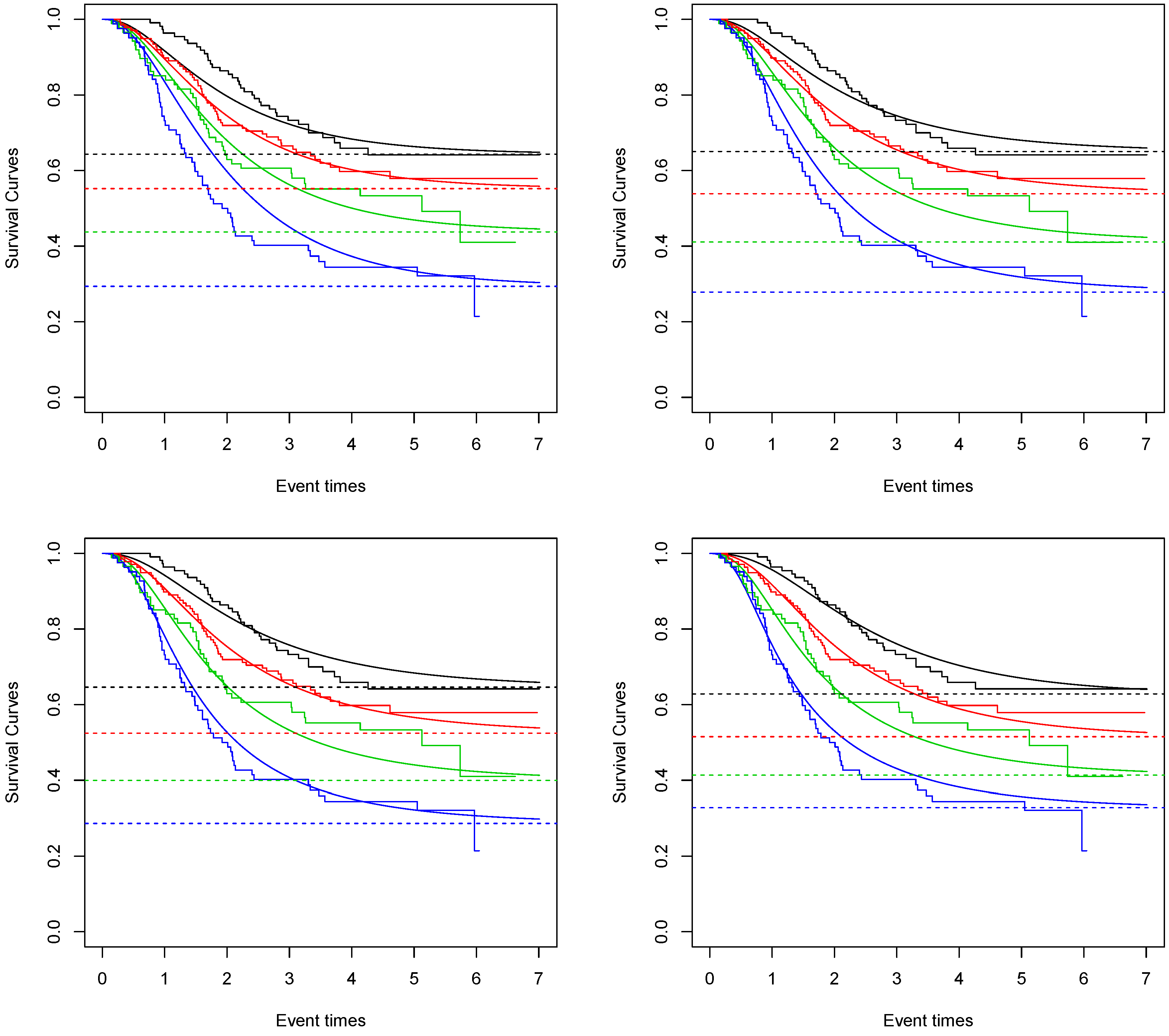
In Figure 1, the fitted survival curves for each nodule category and each proposed model are given. We can see that the one that best captures the Kaplan–Meier curve is the Negative Binomial Kumaraswamy Exponential distribution. This result is also sustained by the AIC values. The values obtained for the Bernoulli, Poisson, Geometric and Negative Binomial Kumaraswamy Exponential models are 1029.53, 1022.77, 1017.64 and 1016.27. The Negative Binomial Kumaraswamy Exponential achieves a better AIC value even with one extra parameter than the others.

Considering the Negative Binomial Kumaraswamy Exponential model and given the average age of 48 in this study, the estimated cure rate for nodule category 1 is around 0.65. For nodule category 2, it is around 0.54. For nodule category 3, it is around 0.41. For nodule category 4, it is around 0.28.

The standard deviations of $p_1$, $p_2$, $p_3$ and $p_4$ are 0.0464, 0.0412, 0.0424 and 0.0525, respectively. The bootstrap 95 percent confidence intervals are (0.55, 0.73), (0.45, 0.61), (0.33, 0.49) and (0.18, 0.38), respectively. These indicate a significant difference between nodule categories 1 and 3, 1 and 4 and 2 and 4. These results agree with the results found in (Rodrigues et al. 2009, Balakrishnan and Pala 2013a, 2013b).

4. Conclusions

We have presented the Kumaraswamy generalized family using the Negative Binomial as the distribution of the latent causes, in a survival analysis context. We exemplified the unified family using the exponential distribution as the baseline distribution. This model has several special cases, such as the standard and promotion time cure rate models. In addition, we consider covariates in a long-term model in order to identify factors that influence the survival function and the cured fraction. A simulation study was performed and showed us that, in addition to the interval estimation that takes relatively large sample sizes to converge, a reasonable point estimate of the cure rate is given even in small sample sizes. We thus have a model that is applicable in many practical cases. Through its application, it was found that the models proposed in this work can be useful in the analysis of health risk data.