Forest Tree Species Classification Based on Sentinel-2 Images and Auxiliary Data

Abstract

Most research on forest tree species classification based on optical image data uses information such as spectral reflectance, vegetation index, texture, and phenology data. However, owing to the limited spectral resolution of multispectral images and the high cost of hyperspectral data, there is room for improvement in the classification of tree species in large areas based on optical images. The combined application of multispectral images and other auxiliary data can provide a new method for improving tree species classification accuracy. Hence, Sentinel-2 images were used to extract spectral reflectance, spectral index, texture, and phenological information. Data for topography, precipitation, air temperature, ultraviolet aerosol index, NO₂ concentration, and other variables were included as auxiliary data. Models for forest tree species classification were constructed through feature combination and feature optimization using the random forest (RF), gradient tree boost (GTB), support vector machine (SVM), and classification and regression tree (CART) algorithms. The classification results of 16 feature combinations with the 4 classification methods were compared, and the contributions of different features to the classification models of forest tree species were evaluated. Finally, the optimal classification model was selected to identify the spatial distribution of forest tree species in the study area. The model based on feature optimization gave the best results among the 16 feature combination models. The overall accuracy and kappa coefficient were increased by 18% and 0.21, respectively, compared with the spectral classification model, and by 17% and 0.20, respectively, compared with the spectral and spectral index classification model. By analyzing the feature optimization model, it was found that terrain, ultraviolet aerosol index, and phenological information ranked as the top three features in terms of importance. Although the importance of spectral reflectance and spectral index features was lower, the number of feature variables accounted for a large proportion of the total. The importance of commonly used texture features was limited, and these features were not present in the feature optimization model. The RF algorithm had the highest classification accuracy, with an overall accuracy of 82.69% and a kappa coefficient of 0.80, among the four classification algorithms. The results of GTB were close to those of RF, and the difference in overall classification accuracy was only 0.14%. However, the results of the SVM and CART algorithms were relatively weaker, with overall classification accuracies of about 70%. It can be concluded that the combined application of Sentinel-2 images and auxiliary data can improve forest tree species classification accuracy. The model based on feature optimization achieved the highest classification accuracy among the 16 feature combination models. The spectral reflectance and spectral index data extracted from optical images are useful for tree species classification, but the effect of texture features was very limited. Auxiliary data, such as topographic features, ultraviolet aerosol index, phenological features, NO₂ concentration features, topographic diversity features, precipitation features, temperature features, and multi-scale topographic location index data, can effectively improve forest tree species classification accuracy. The RF algorithm had the highest accuracy, and it can be used for tree species classification space distribution identification. The combined application of Sentinel-2 images and auxiliary data can improve classification accuracy, but the highest accuracy of the model was only 82.69%, which leaves room for improvement. Thus, more effective auxiliary data and the vertical structural parameters extracted from satellite LiDAR can be combined with multispectral images to improve forest tree species classification accuracy in future research.

1. Introduction

As the main component of the terrestrial ecosystem, forests play a vital role in regulating global climate and maintaining biodiversity, ecological balance, and the global carbon and water cycles [1,2]. Tree species are key parameters in characterizing forest ecosystems, and they not only provide an important basis for forest planning, design, operation, and management but are also important parameters for a variety of ecological process simulations [3]. Hence, how to accurately and efficiently obtain quantity and distribution information for forest tree species is a crucial problem that needs to be solved in the domains of scientific management and effective utilization of forest resources.

The main traditional forest resources survey method is the ground survey, but it has a high cost, long cycle, and large workload, and it does not provide detailed spatial distribution information for forest tree species types, which is a need of modern forestry resource management. Remote sensing can overcome the shortcomings of traditional forest resource surveys, and it has been widely used in the classification research of forest tree species [4]. Based on GF-6 images, Huang et al. [5] used the random forest (RF) machine learning method to classify forest tree species, such as eucalyptus, pine trees, cedar, and other arbor forests, by calculating the vegetation index and optimizing the feature combination. The results showed that the model of optimized feature combination was the best, with an accuracy of 85.38%. The accuracy was higher by 3.98% and 8.97% compared to the model of red edge bands and the model of non-red edge bands, respectively. Based on airborne hyperspectral data, Zhao et al. [6] used a 3D convolutional neural network to classify forest tree species, such as cedar, pine trees, eucalyptus, and mytilaria, in the Nanning Gaofeng Forest Farm of Guangxi in China. The overall classification accuracy was 98.38%, and the kappa coefficient was 0.90. Based on multi-phase Sentinel-2 data, Immitzer et al. [7] used the RF algorithm to classify 12 tree species of a Central European forest with an overall accuracy of 89%. Based on hyperspectral data, Zhao et al. [8] classified seven tree species of a shelter forest using maximum likelihood, support vector machine (SVM), and RF algorithms. The result showed that the overall accuracy of the RF algorithm was 95.93%, and the kappa coefficient was 0.95. Through analysis of previous forest tree species classification studies, it was found that the main optical satellite images used were multispectral and hyperspectral images, and the classification accuracy of hyperspectral images was usually higher than that of multispectral images. However, hyperspectral images are more commonly used in small areas; it is difficult to use them for large areas owing to the complexity of data processing and the high cost. Multispectral imagery is usually available for free and is simple to process; therefore, it is commonly used in large-area studies. However, due to the relatively small number of bands and limited spectral resolution, the classification results for different tree species need to be further improved. How to effectively use auxiliary data to make up for the insufficiency of multispectral images and then improve the classification results is an active area of research related to forest tree species classification.

To improve the classification results of forest tree species, researchers have tried to apply multispectral image data together with other data and have achieved good results. For example, Hoscilo et al. [9] used multi-time Sentinel-2 data and topographic information to classify forest tree species in large areas. The results showed that topographic variables played a significant role in tree species classification, and the introduction of topographic variables increased the classification accuracy from 75.60% to 81.70%. Ma et al. [10] classified forest tree species in the eastern part of the Qilian Mountains based on Sentinel-2 spectral features, texture features, and topographic features. The results showed that the combination of elevation, slope, slope aspect, and texture features can increase the separation of tree species, with an overall accuracy of 86.49% and a kappa coefficient of 0.83. Cai et al. [11] used RF, SVM, and XGboost to classify the four main dominant tree species in Longquan City, namely, broad-leaved trees, pine trees, Chinese fir, and Moso bamboo, based on the spectral reflectance, texture, and spectral index information extracted from Gaofen-2 data along with topographic characteristics data. The highest accuracy was achieved with the XGboost algorithm (83.88%), and the kappa coefficient was 0.78. Tran et al. [12] used an object-oriented classification method to classify broad-leaved deciduous forest tree species, including mixed semi-evergreen forest, keruing, dark red meranti, and sal, based on phenological information and the backscattering coefficient extracted from the Landsat-8 and Sentinel-1 time-series images. The overall classification accuracy was about 79%, and the kappa coefficient was 0.70. Previous research results show that the combined application of multi-source data can overcome the shortcomings of multispectral images and improve classification accuracy. However, the auxiliary data used in former research are mostly topographic factors and phenological information. Besides the topographic factors and phenological information, other auxiliary data are also closely related to the distribution of forest tree species. For example, precipitation and temperature will affect the distribution area of different tree species. Through field surveys, it was found that eucalyptus often grows in warmer regions, while cedars are suited to growing in relatively cold temperatures. The distributions of different tree species also change with air quality. Population densities and administrative unit areas also restrict the distributions of forests. However, in the former research, the closely related auxiliary data have been little researched regarding their influence on the classification of forest tree species. Therefore, in this paper, more variables, such as topography, precipitation, air temperature, ultraviolet aerosol index, NO₂ concentration, topographic diversity, multi-scale topographic location index, and others, were chosen as auxiliary data to combine with Sentinel-2 data to improve the accuracy of forest tree species classification.

In addition to the auxiliary data, the algorithm is also an important factor affecting the accuracy of tree species classification. With their excellent performance, machine learning algorithms have been widely used in classification research in the past decades. For example, Hologa et al. [13] used the RF algorithm to classify tree species in temperate mixed mountains based on multiple datasets, and the highest overall accuracy was 89.50%. Hu et al. [14] used an SVM algorithm to classify tree species based on multi-source remote sensing data, and the overall classification accuracy was 89%. Chen et al. [15] used a CART algorithm to classify tree species based on QuickBird image, with an overall accuracy of 80.50%. Previous research results show that machine learning algorithms, such as RF, SVM and CART, can realize tree species classification. As a machine learning algorithm, GTB is an ensemble learning method, whose base model is also a tree model. It can reduce the variance of the overall model by random sampling of features and flexibly process various types of data, including continuous values and discrete values. Compared to other machine learning algorithms, the GTB algorithm is considered to have the best robustness and not too much time is needed for the tuning of parameters; the results of the model are still relatively good [16,17,18]. However, GTB is seldom used in forest tree classification research; therefore, the performance of GBT in forest tree species classification is still unknown.

The objectives of this study were as follows: (i) to investigate the influence of other auxiliary data besides topographic factors and phenological information, such as precipitation, air temperature, ultraviolet aerosol index, NO₂ concentration, topographic diversity, multi-scale topographic location index, and other variables, on forest tree species classification; (ii) to investigate the performance of four machine learning algorithms (RF, GTB, SVM, and CART) on forest tree species classification and choose the most suitable algorithm for forest tree species classification; and (iii) to improve the accuracy of forest tree species classification through feature optimization based on the combined application of Sentinel-2 and auxiliary data.

2. Study Area and Data

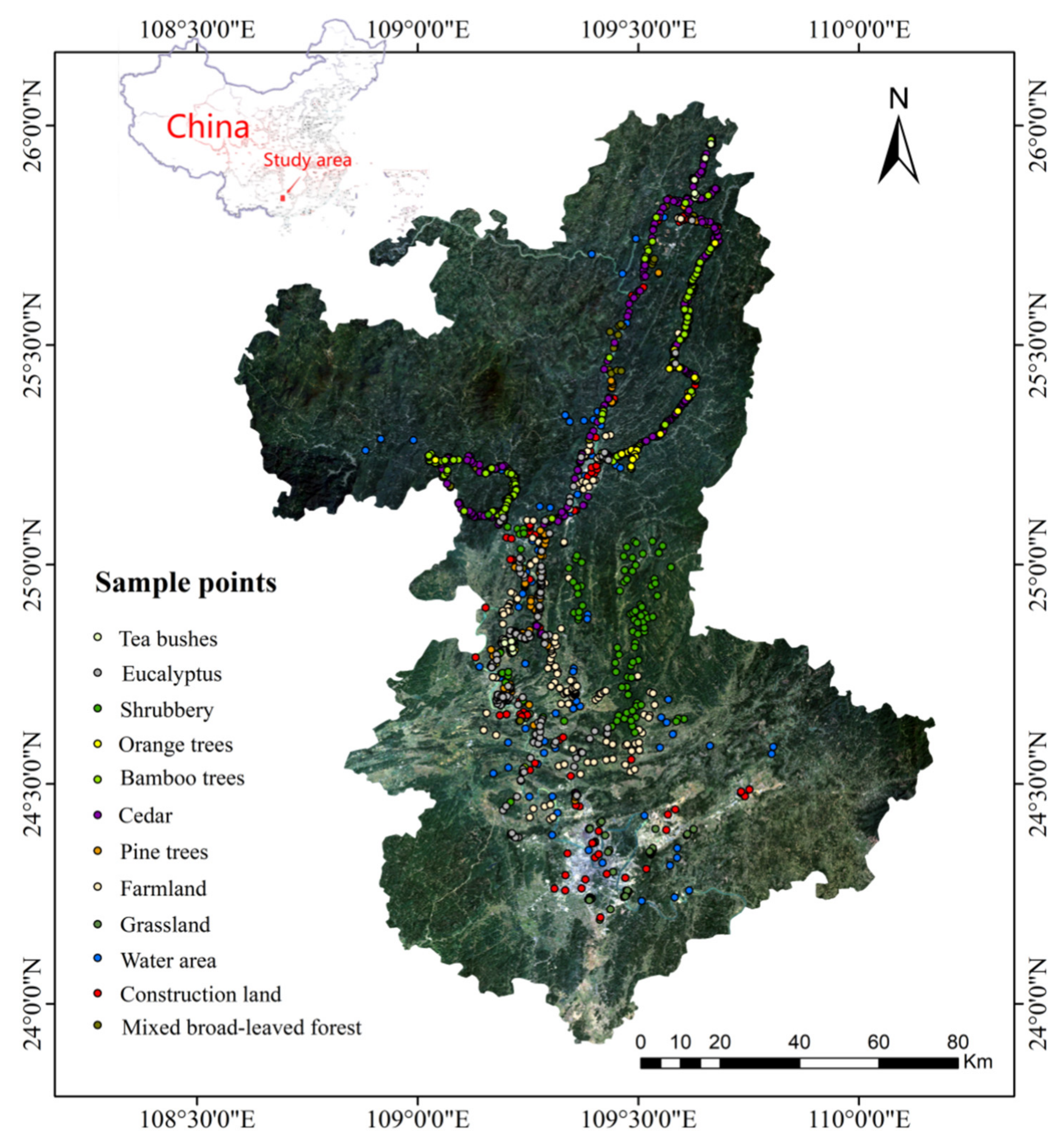
2.1. Study Area

The study area was located in Liuzhou city, Guangxi Zhuang Autonomous Region, China (108°32′–110°28′ E, 23°54′–26°03′ N) (Figure 1). This area is karst terrain, with an elevation ranging from 85 m to 150 m. The climate is a subtropical monsoon climate, with an average annual temperature of 20.5 °C, annual rainfall of 1400–1500 m, annual sunshine of more than 1600 h, and a frost-free period of more than 300 days. The forest coverage rate is 66.70%, and most of the forests are planted forests. The existing broad-leaved forests mainly include Eucalyptus (Eucalyptus robusta Smith), orange trees (Citrus reticulate L.), tea bushes (Camellia sinensis (L) Kuntze), bamboo trees (Phyllostachys edulis (Carriere) J. Houzeau), shrubbery, and natural mixed broad-leaved forest; the coniferous forests are mainly cedar (Cunninghamia lanceolata (Lamb.) Hook) and pine tree forests (Pinus L.).

2.2. Data

2.2.1. Sentinel-2 Data

Sentinel-2 is a wide, high-resolution, multispectral imaging satellite with a revisit frequency of 5 days and 12 spectral bands. There are four bands of visible light and near-infrared with a spatial resolution of 10 m, six bands of red edge and short-wave infrared with a spatial resolution of 20 m, and two atmospheric bands with a spatial resolution of 60 m. The Sentinel-2 images used in this study were Level-2A images from 2020, which had been subjected to atmospheric correction and radiometric calibration. To avoid the influence of cloud coverage on the classification results, images with cloud coverage less than 5% were selected for subsequent mosaic mask processing. The images were resampled to 10 m.

2.2.2. Auxiliary Data

The auxiliary data used in the study were digital elevation data, precipitation data, temperature data, water data, Sentinel-5P ultraviolet aerosol index data, multi-scale topographic position index data, topographic diversity data, population density data, Sentinel-5P carbon dioxide data, and mean administrative unit area data. All the above data were obtained through Google Earth Engine (GEE), and the spatial resolution of all auxiliary data was resampled to 10 m. Detailed descriptions of the auxiliary data are presented in

Table 1. The auxiliary data used in this study.

Dataset	GEE ID	Dataset Provider	Period	Spatial Resolution
Emissivity 8-Day Global 1 km SRTM Digital Elevation Data (digital elevation data)	USGS/SRTMGL1_003	NASA/USGS/JPL-Caltech	2000	30 m
CHIRPS Daily: Climate Hazards Group InfraRed Precipitation with Station Data (V 2) (precipitation data)	UCSB-CHG/CHIRPS/DAILY	UCSB/CHG	1 January 1981–30 June 2022	5566 m
GCOM-C/SGLI L3 Land Surface Temperature (V2) (temperature data)	JAXA/GCOM-C/L3/LAND/LST/V2	Global Change Observation Mission	1 January 2018–28 November 2021	4638.3 m
JRC Monthly Water History, v1.3 (water data)	JRC/GSW1_3/MonthlyHistory	EC JRC/Google	16 March 1984–1 January 2021	30 m
Sentinel-5P NRTI AER AI: Near Real-Time UV Aerosol Index (Sentinel-5P ultraviolet aerosol index data)	COPERNICUS/S5P/NRTI/L3_AER_AI	European Union/ESA/Copernicus	10 July 2018–15 August 2022	1113.2 m
Global ALOS mTPI (multi-scale topographic position index data)	CSP/ERGo/1_0/Global/ALOS_mTPI	Conservation Science Partners	24 January 2006–13 May 2011	270 m
Global ALOS Topographic Diversity (topographic diversity data)	CSP/ERGo/1_0/Global/ALOS_topoDiversity	Conservation Science Partners	24 January 2006–13 May 2011	270 m
GPWv411: Population Density (V 4) (population density data)	CIESIN/GPWv411/GPW_Population_Density	NASA SEDAC at the Center for International Earth Science Information Network	1 January 2000–1 January 2020	927.67 m
Sentinel-5P OFFL NO2: Offline Nitrogen Dioxide (Sentinel-5P carbon dioxide data)	COPERNICUS/S5P/OFFL/L3_NO2	European Union/ESA/Copernicus	28 June 2018–6 August 2022	1113.2 m
GPWv411: Mean Administrative Unit Area (V 4) (mean administrative unit area data)	CIESIN/GPWv411/GPW_Mean_Administrative_Unit_Area	NASA SEDAC at the Center for International Earth Science Information Network	1 January 2000–1 January 2020	927.67 m

.

2.2.3. Field Survey Data

The sample data used in the study were from a field survey undertaken in 2021 and included high-resolution images obtained through Google Earth Pro. According to the field survey, the forest tree species in the study area mainly included eucalyptus, cedar, pine trees, orange trees, tea bushes, bamboo trees, shrubbery, and mixed broad-leaved forest. The non-forest land cover mainly included farmland, water area, grassland, and construction land. A total of 1481 sample points were selected in the study area. The spatial distribution and specific quantities of the sample points are shown in Figure 1 and

Table 2. Category and quantity of sample points.

Type	Category of Sample Points	Quantity of Sample Points
Forest land	Eucalyptus	148
	Bamboo trees	164
	Pine trees	122
	Cedar	407
	Orange trees	51
	Tea bushes	47
	Brushwood	107
	Mixed broad-leaved forest	85
Non-forest land	Water area	80
	Farmland	139
	Construction land	74
	Grassland	57

, respectively.

3. Methods

In this paper, the Sentinel-2 images were processed to extract various features, including spectral reflectance features, phenological features, spectral indices, and texture features. More data, such as topography, precipitation, air temperature, ultraviolet aerosol index, NO₂ concentration, topographic diversity, multi-scale topographic lo-cation index, and other variables, were used as auxiliary data. Models of forest tree species classification were constructed with four commonly used algorithms (RF, GTB, CART, and SVM) based on the features extracted from Sentinel-2 images and auxiliary data. The accuracy of models was assessed with 10-fold cross-validation based on the field survey data. The classification results of different feature combinations with the four algorithms were compared, and the optimal classification model was selected to identify the spatial distribution of forest tree species in the study area. The flowchart used in this study is shown in Figure 2.

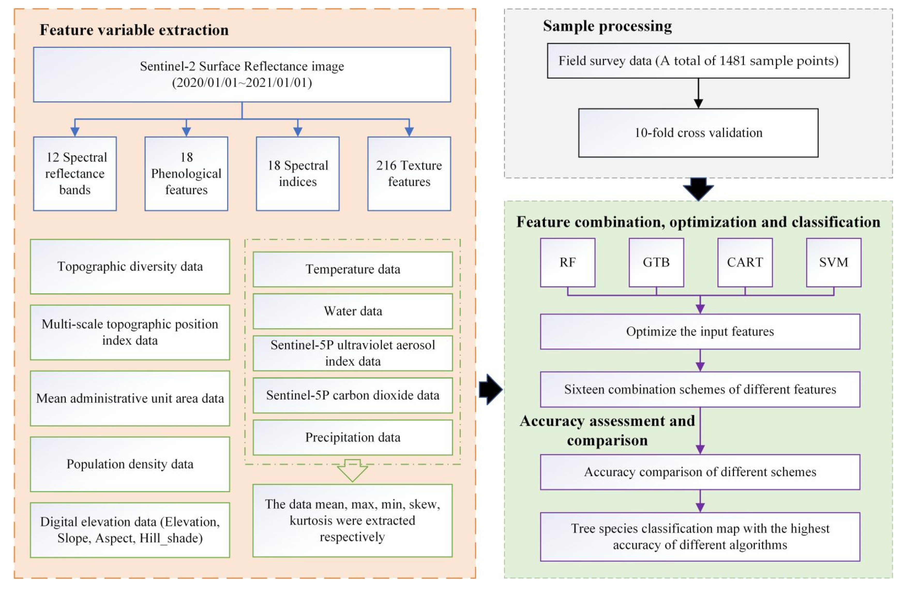
3.1. Feature Combination Scheme

To quantify the impact of different characteristic variables on the classification results of the forest tree species, the spectral reflectance data extracted from Sentinel-2 imagery were used as the basic data, and 16 combination schemes of different features were used to construct the classification model (

Table 3. Sixteen combination schemes of different features.

Scheme	Feature Combination
1	Spectral features
2	Spectral features + spectral indices
3	Spectral features + texture features
4	Spectral features + temperature features
5	Spectral features + precipitation features
6	Spectral features + terrain features
7	Spectral features + phenological features
8	Spectral features + water features
9	Spectral features + population density feature
10	Spectral features + topographic diversity feature
11	Spectral features + multi-scale topographic position index
12	Spectral features + ultraviolet aerosol indices
13	Spectral features + NO2 concentration features
14	Spectral features + administrative unit area feature
15	Spectral features + all of the above features
16	Preference features

).

3.2. Feature Variable Extraction

Sentinel-2 images and auxiliary data were resampled, and the corresponding feature variables were extracted from the resampled Sentinel-2 images and auxiliary data based on the 16 feature combination schemes. The specific feature variables of different features are shown in

Table 4. Specific feature variables of different features.

Features	Number	Feature Variable
Spectral features	12	B1, B2, B3, B4, B5, B6, B7, B8, B8A, B9, B11, B12
Spectral indices	18	EVI, NDVI, NDVIA, MTCI, IRECI, PSRI, TCARI, NDWI, MCARI, RDVI, TVI, SAVI, MSI, LSWI, NDVIred_edge, mNDVIred_edge, MSRred_edge, CIred_edge
Texture features	216	The texture metric was calculated from the gray level co-occurrence matrix around each pixel in each band. Each band yielded 18 texture feature variables. There were a total of 216 feature variables
Temperature features	5	Temp_mean, Temp_max, Temp_min, Temp_skew, Temp_kurtosis
Precipitation features	5	Precipitation_mean, Precipitation_max, Precipitation_min, Precipitation_skew, Precipitation_kurtosis
Terrain features	4	Elevation, Slope, Aspect, Hill_shade
Phenological features	18	NDVI_winter, NDVI_summer, NDVI_spring, NDVI_fall, EVI_winter, EVI_summer, EVI_spring, EVI_fall, LSWI_winter, LSWI_summer, LSWI_spring, LSWI_fall, NDVI_summer_winter, NDVI_fall_spring, EVI_summer_winter, EVI_fall_spring, LSWI_summer_winter, LSWI_fall_spring
Water features	5	Water_mean, Water_max, Water_min, Water_skew, Water_kurtosis
Population density feature	1	PD
Topographic diversity feature	1	TD
Multi-scale topographic position index	1	MSTPI
Ultraviolet aerosol indices	5	Aerosol_mean, Aerosol_max, Aerosol_min, Aerosol_skew, Aerosol_kurtosis
NO2 concentration features	5	NO2_mean, NO2_max, NO2_min, NO2_skew, NO2_kurtosis
Administrative unit area feature	1	MAUA

, and the calculation formulas for the spectral index feature variables are shown in

Table 5. Calculation formulas for the spectral index feature variables.

Spectral Indices	Formula	Reference
Enhanced vegetation index (EVI)	2.5 × (B8 − B4)/(B8 + 6 × B4 − 7.5 × B2 + 1)	Liu et al. [19]
Normalized difference vegetation index (NDVI)	(B8 − B4)/(B8 + B4)	Broge et al. [20]
Normalized difference vegetation index (NDVIA)	(B8A − B4)/(B8A + B4)	Broge et al. [20]
MERIS terrestrial chlorophyll index (MTCI)	(B6 − B5)/(B5 − B4)	Dash et al. [21]
Inverted red-edge chlorophyll index (IRECI)	(B7 − B4)/(B5/B6)	Frampton et al. [22]
Plant senescence reflectance index (PSRI)	(B4 − B3)/B6)	Merzlyak et al. [23]
Transformed chlorophyll absorption in reflectance index (TCARI)	3 × ((B8 − B4) − 0.2 × (B8 − B3)) × (B8/B4)	Haboudane et al. [24]
Normalized difference water index (NDWI)	(B3 − B8)/(B8 + B3)	Mcfeeters et al. [25]
Modified chlorophyll absorption in reflectance index (MCARI)	(B8 − B4) − 0.2 × (B8 − B3)) × (B8/B4)	Daughtry et al. [26]
Ratio difference vegetation index (RDVI)	(B8 − B4)/pow (B8 − B4,0.5)	Huete et al. [27]
Triangular vegetation index (TVI)	0.5 × (120 × (B8 − B3)/200 × (B4 − B3))	Broge et al. [28]
Soil adjusted vegetation index (SAVI)	(1 + 0.2) × float (B8 − B4)/(B8 + B4 + 0.2)	Bolyn et al. [29]
Moisture stress index (MSI)	B8/B3	Bolyn et al. [29]
Land surface water index (LSWI)	(B8 − B11)/(B8 + B11)	Bridhikitti et al. [30]
Normalized difference red-edge vegetation index (NDVIred_edge)	(B6 − B5)/(B6 + B5)	Gamon et al. [31]
Modified normalized difference red-edge vegetation index (mNDVIred_edge)	(B6 − B5)/(B6 + B5 – 2 × B1)	Le Maire et al. [32]
Modified specific ratio red-edge vegetation index (MSRred_edge)	(B6 − B1)/(B5 + B1)	Fourty et al. [33]
Chlorophyll red-edge index (CIred_edge)	(B6 − 800/B5 − 725) − 1	Gitelson et al. [34]

.

3.3. Classification Algorithm

Based on the feature combination schemes and feature variable extraction, four commonly used machine learning algorithms, namely, RF, GTB, CART, and SVM, were used for forest tree species classification. The classification algorithms are summarized below.

(1) The RF algorithm is an ensemble algorithm, which belongs to the bagging type. It integrates the results of a large number of regression trees. It outputs the predicted class for classification or mean predicted value for regression by constructing a large number of decision trees during training. The majority “vote” among all trees is used to assign a final class to each unknown tree, so that the results of the overall model have high accuracy and generalization potential. RF corrects the overfitting problem of the decision tree algorithm. The relative importance of each band can be evaluated by systematically comparing the performances of trees with and without specific bands [35].

(2) The GTB method is a tree ensemble model in which the subsamples of training data for each iteration are randomly selected from the complete training data. This subsample is then used to fit the base learner and update the model for the next iteration, gradually reducing the cumulative model loss [36]. In other words, gradient descent in parameter space uses gradient information to adjust parameters to reduce the loss, and gradient descent in the function space uses a gradient to fit a new function to reduce the loss. GTB is a boosting algorithm for decision trees, which is one of the best algorithms for fitting the real distribution in traditional machine learning algorithms. It is a strong classifier, which is generally more accurate than a decision tree, and can choose the loss function by itself. Compared to the SVM algorithm, the prediction accuracy of GTB can also be relatively high with relatively less time taken for parameter adjustment.

(3) CART is a decision tree algorithm. It is a learning method that outputs the conditional probability distribution of a random variable under the condition of given input random variables. CART determines the relationship between a single continuous response and multiple continuous and/or discrete explanatory variables through a bivariate recursive partitioning process, in which the data are repeatedly split into increasingly uniform groups, using the combination of variables that best distinguishes changes in the response variables [37]. The CART algorithm is very stable in the face of problems, such as missing values and too many variables.

(4) SVM is a set of related supervised learning methods that are widely used in data analysis and pattern recognition for classification and regression analysis. The basic principle of SVM is to map the input vectors onto a high-dimensional feature space through pre-selected nonlinear relations and find an optimal classification hyperplane in this space to maximize the classification interval between two classes. The most commonly used SVM is the linear classifier, which can predict the member classification of each input between two possible classifications. It classifies all inputs by building a hyperplane or a set of hyperplanes in a high-dimensional or even an infinite space. The value closest to the classification margin is called a support vector [38].

3.4. Accuracy Assessment

To prevent errors caused by sample selection, 10-fold cross-validation was used. The accuracy assessment indicators were the user’s accuracy (UA), the producer’s accuracy (PA), overall accuracy (OA), and the kappa coefficient. The calculation formulas are as follows:

$$U{A}_i=\frac{p_{ii}}{p_{i+}},$$

(1)

$$P{A}_i=\frac{p_{ii}}{p_{+i}},$$

(2)

$$OA=\frac{{\displaystyle {\sum }_{i=1}^k{p}_{ii}}}{p},$$

(3)

$$Kappa=\frac{p{\displaystyle \sum {}_{i=1}^k{p}_{ii}-{\displaystyle \sum {}_{i=1}^k{p}_{i+}{p}_{+i}}}}{p^2-{\displaystyle \sum {}_{i=1}^k{p}_{i+}{p}_{+i}}},$$

(4)

where p is the total number of samples; k is the total number of categories; p_ii is the number of samples correctly classified; p_+i is the number of samples of category i; and p_i+ is the number of samples predicted as category i.

4. Results

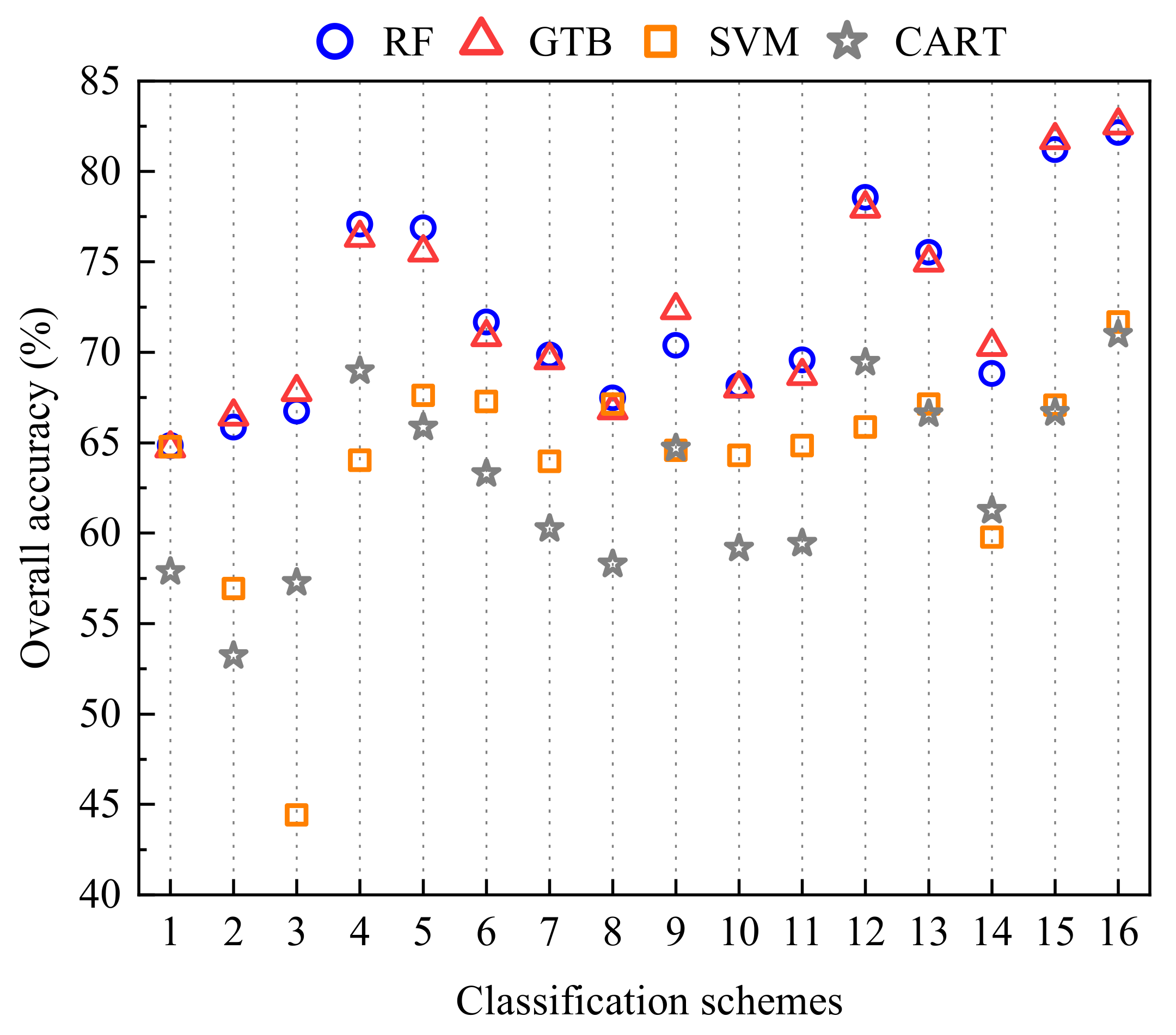
4.1. Classification Results with Different Feature Combination Schemes

The accuracy of the results for the 16 different feature combination schemes is shown in Figure 3. It can be seen from the figure that the RF, GTB, SVM, and CART classification algorithms all achieved the highest classification accuracies with scheme 16 (preference feature combination). The overall accuracy of the RF and GTB results was high at about 82.50%, and the accuracy of the classification results for SVM and CART was relatively low at about 72%, which is about 10% lower.

Compared with the classification results of scheme 1 (spectral features), the classification results of scheme 4 (spectral features + temperature features), scheme 5 (spectral features + precipitation features), and scheme 12 (spectral feature + ultraviolet aerosol indices) were significantly better. The results show that the temperature, precipitation, and ultraviolet aerosol index features can make up for the fewer bands of multispectral images and improve the accuracy of forest tree species classification. For the commonly used features of multispectral images, such as spectral index and texture information, the improvement in classification results is limited and may even be negative. For example, the maximum improvement of the RF and GTB algorithms was only 3.10%, and with the SVM and CART algorithms the accuracy of the classification results decreased, with the maximum decrease being 20.30%. The results show that the introduction of inappropriate features may reduce the accuracy of classification. The results of schemes 15 and 16 also confirm this conclusion. Therefore, it is necessary to properly optimize the features used for tree species classification.

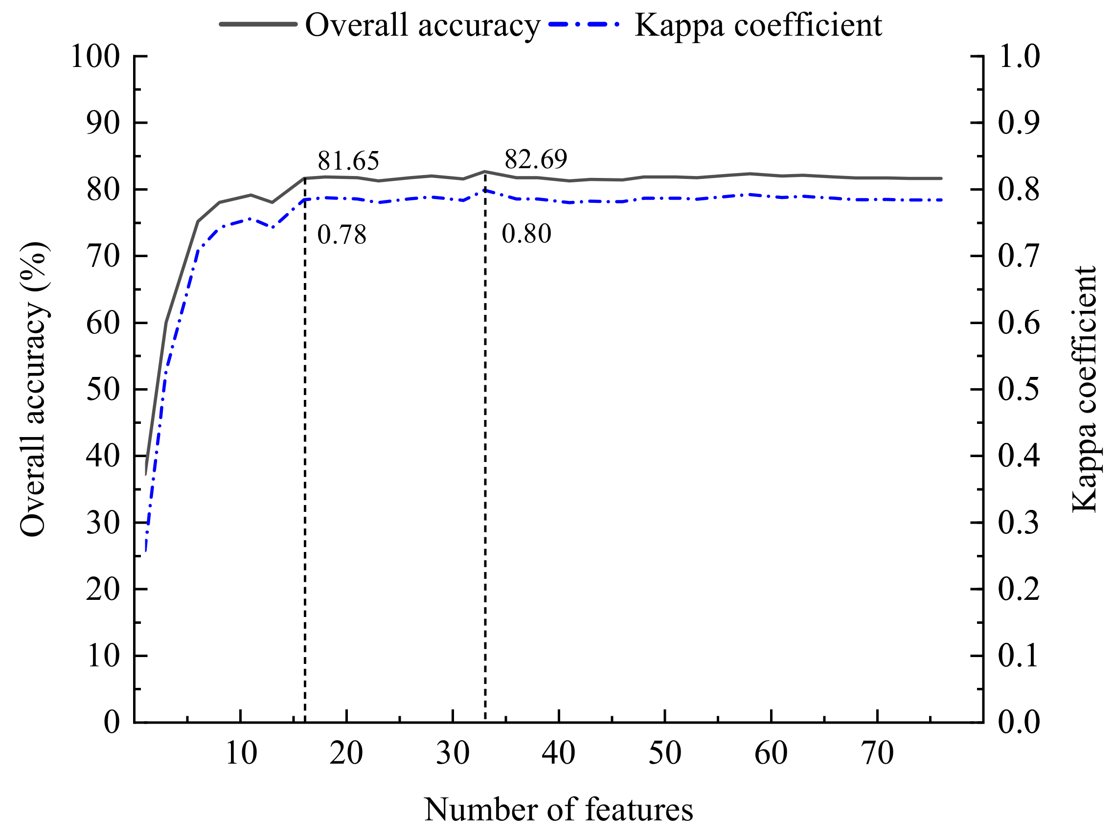
4.2. Analysis of Feature Variable Optimization Results

The results shown in Figure 3 demonstrate that different features can provide more information for tree species classification. However, the increase in the number of features will not only cause informational redundancy and higher data calculation costs but also reduce the accuracy of classification [39]. Therefore, it is very important to optimize the input features. Based on the classification results of the four algorithms, the RF algorithm provided the best results under different feature combinations. Therefore, the RF algorithm is used as an example to show the optimization of feature variables on the basis of scheme 15. The importance score ranking of each feature variable is shown in

Table 6. Table of the 79 feature variable importance scores.

Number	Feature Variable	Score	Number	Feature Variable	Score	Number	Feature Variable	Score
1	Elevation	70.96	28	B11	55.96	55	MCARI	49.62
2	Aerosol_skew	67.77	29	NO2_min	55.83	56	B3	49.37
3	LSWI_summer	65.69	30	NO2_max	55.38	57	Precipitation_kurtosis	49.13
4	Aerosol_mean	65.53	31	MSTPI	55.09	58	MSI	48.85
5	Aerosol_kurtosis	63.85	32	NDVI_summer	54.72	59	Aerosol_min	48.43
6	PSRI	63.06	33	NDVIred_edge	54.58	60	MAUA	48.26
7	NO2_mean	62.58	34	EVI_fall	54.53	61	NDVI	48.16
8	LSWI_fall	61.76	35	NDVIA	54.11	62	Hill_shade	48.06
9	B5	61.34	36	CIred_edge	53.94	63	B4	47.87
10	B9	61.22	37	PD	53.72	64	B7	47.27
11	Temp_mean	60.71	38	NDWI	53.67	65	Temp_kurtosis	46.34
12	Precipitation_mean	60.31	39	LSWI_winter	53.39	66	NO2_skew	45.75
13	EVI_spring	59.76	40	NO2_kurtosis	53.23	67	SAVI	45.62
14	B12	58.92	41	NDVI_winter	53.06	68	IRECI	45.24
15	MTCI	58.28	42	B8	52.94	69	TCARI	45.09
16	B6	57.69	43	LSWI	52.92	70	Temp_skew	45.09
17	B2	57.63	44	Slope	52.85	71	EVI	44.50
18	TD	57.23	45	NDVI_summer_winter	52.57	72	Precipitation_max	44.48
19	B1	57.21	46	Precipitation_skew	52.30	73	B8A	44.36
20	RDVI	57.09	47	MSRred_edge	52.25	74	EVI_fall_spring	44.04
21	LSWI_spring	57.01	48	NDVI_fall_spring	51.65	75	Temp_min	38.54
22	mNDVIred_edge	56.92	49	Aerosol_max	51.54	76	Water_skew	32.71
23	LSWI_summer_winter	56.90	50	EVI_summer_winter	51.41	77	Water_mean	29.75
24	LSWI_fall_spring	56.71	51	Aspect	51.26	78	Water_kurtosis	26.95
25	NDVI_spring	56.47	52	EVI_winter	51.18	79	Water_max	1.99
26	EVI_summer	56.27	53	TVI	49.93
27	Temp_max	56.05	54	NDVI_fall	49.86

. The importance score is 0 from the 80th feature variable onward; so, the feature variables after 80 are excluded and only the preceding 79 feature variables are displayed. As shown in Table 6, the texture features were not in the 79 feature variables; so, those features can be excluded.

With the addition of feature variables, the results of the model decrease slightly and then continue to increase. When the number of feature variables is 16, the changes in the overall accuracy and kappa coefficient of the model are relatively small and tend to be stable. At this time, the overall accuracy and kappa coefficient of the model are 81.65% and 0.78, respectively. When the number of feature variables reaches 33, the overall accuracy and kappa coefficient are highest, at 82.69% and 0.80, respectively. After that, the addition of feature variables does not improve the classification results. Therefore, the preceding 33 feature variables (feature combination scheme 16) were chosen as the final preferred feature variables for the RF algorithm.

Based on the results shown in Table 6 and Figure 4, the 33 preferred feature variables consisted of 1 topographic feature variable (Elevation), 3 ultraviolet aerosol index feature variables (Aerosol_skew, Aerosol_mean, and Aerosol_kurtosis), 9 phenological feature variables (LSWI_summer, LSWI_fall, EVI_spring, LSWI_spring, LSWI_summer_winter, LSWI_fall_spring, NDVI_spring, EVI_summer, EVI_summer, and NDVI_summer), 5 spectral index feature variables (PSRI, MTCI, RDVI, mNDVIred_edge, and NDVIred_edge), 3 NO₂ concentration feature variables (NO2_mean, NO2_max, and NO2_min), 7 spectral feature variables (B5, B9, B12, B6, B2, B1, and B11), 1 topographic diversity feature variable (TD), 1 precipitation feature variable (Precipitation_mean), 2 temperature feature variables (Temp_mean and Temp_max), and 1 multi-scale topographic position index feature variable (MSTPI). The results show that 10 features (including topographic features, ultraviolet aerosol index features, and phenology features) can improve the results of forest tree species classification.

The same operation of feature variable optimization was performed for the GTB, CART, and SVM algorithms. Fifteen feature variables along with their importance score ranks are shown in

Table 7. Fifteen feature variables along with the importance score ranks for the four algorithms.

Number	RF	SVM	CART	GTB
	Feature Variables
1	Elevation	TD	B1	B11
2	Aerosol_skew	LSWI_fall_spring	Elevation	B1
3	LSWI_summer	Temp_skew	B9	NO2_mean
4	Aerosol_mean	NDVI_fall	MTCI	MAUA
5	Aerosol_kurtosis	B8	MSRred_edge	Elevation
6	PSRI	NDVI_fall_spring	B2	B9
7	NO2_mean	B7	PSRI	Slope
8	LSWI_fall	B8A	LSWI	LSWI_summer
9	B5	B11	Slope	mNDVIred_edge
10	B9	NDVI_summer_winter	NDVI	B12
11	Temp_mean	LSWI_summer_winter	EVI_fall	NDVI_winter
12	Precipitation_mean	mNDVIred_edge	EVI	AVE
13	EVI_spring	LSWI	EVI_winter	Aerosol_kurtosis
14	B12	MSRred_edge	mNDVIred_edge	NO2_max
15	MTCI	B12	PD	Aerosol_mean

. By analyzing the results shown in Table 7, it can be seen that the categories of the 15 feature variables are approximately the same: spectral features, topographic features, spectral indices, phenological features, ultraviolet aerosol indices, and NO₂ concentration features. The GTB, CART, and SVM algorithms achieved the highest overall accuracy levels when the numbers of feature variables were 27, 19, and 31, respectively. These were used for the optimal feature combination scheme 16.

To explore why the feature variables affected the classification results, four different feature variables (Elevation, Aerosol_skew, LSWI_summer, and PSRI in Table 7) were selected to analyze the distribution characteristics of different tree species, using the classification results of the RF algorithm with scheme 16 as an example. The results are shown in Figure 5.

The distribution characteristics of the Elevation feature variables of the different tree species are shown in Figure 5a. Orange trees, eucalyptus, tea bushes, and pine trees are mainly distributed in the elevation range from 0 to 400 m; bamboo trees, mixed broad-leaved forest, and cedar are mainly distributed in the elevation range higher than 400 m; and shrubbery is relatively evenly distributed in each elevation range. The results show that different tree species can be approximately divided into three categories through the Elevation feature variable.

The distribution characteristics of the Aerosol_skew feature variables of the different tree species are shown in Figure 5b. The Aerosol_skew indices for cedar, tea bushes, orange trees, bamboo trees, and mixed broad-leaved forest are mostly in the range of −0.50 to 0.30, and those for eucalyptus, pine trees, and shrubbery are in the range of 0.30 to 0.90. The results show that different tree species can be approximately divided into two categories through the Aerosol_skew feature variable.

The distribution characteristics of the LSWI_summer feature variables of the different tree species are shown in Figure 5c. The LSWI_summer indices for cedar, eucalyptus, pine trees, tea bushes, and mixed broad-leaved forest are mostly in the range of 0.24 to 0.36; those for bamboo trees and shrubbery are mainly in the range of 0.12 to 0.30; and those for orange trees are mainly in the range of 0.12 to 0.24. The results show that different tree species can be approximately divided into three categories through the LSWI_summer feature variable.

The distribution characteristics of the PSRI feature variables of the different tree species are shown in Figure 5d. The PSRIs for cedar, tea bushes, pine trees, shrubbery, bamboo trees, and mixed broad-leaved forest are mainly in the range of −0.11 to −0.06, and the PSRI distribution ranges for orange trees and eucalyptus are wide, ranging from −0.09 to 1.11. There is a large distribution area between −0.04 and 1.11. The results show that different tree species can also be approximately divided into two categories through the PSRI feature variable.

To summarize, different tree species can be approximately separated by superposition analysis of the classification results of the different tree species corresponding to the above-mentioned different feature variables. Based on the above analysis results, eucalyptus was taken as an example, as shown in Figure 6. It can be seen from the figure that eucalyptus, pine trees, tea bushes, and orange trees can be divided into one category through the Elevation feature variable. Eucalyptus, shrubbery, and orange trees can be divided into one category through the Aerosol_skew feature variable. The intersection of the two types of data superposition can divide eucalyptus and orange trees into one category. Then, the superposition analysis was performed between the results of the LSWI_summer feature variable and the above results, and it was found that their intersection could distinguish eucalyptus separately.

4.3. Comparison of the Classification Results of Different Algorithms Based on the Optimal Feature Variables

The classification results of different algorithms based on the optimal feature variables are shown in

Table 8. Fifteen feature variables with the importance score ranks for the four algorithms.

	RF	GTB	SVM	CART
Overall accuracy	82.69%	82.55%	71.67%	70.99%
Kappa coefficient	0.80	0.80	0.67	0.66

and Figure 7.

By analyzing Table 8, it can be seen that the classification accuracy of the RF algorithm was the highest and that the classification accuracy of the GTB algorithm was similar to that of the RF algorithm. Their overall accuracy scores were 82.55% and 82.69%, respectively, and the kappa coefficients were 0.80 and 0.80, respectively. The classification results of the SVM and CART algorithms were relatively weaker. Their overall accuracy scores were 11.02% and 11.70% lower, respectively, than the RF algorithm, and the kappa coefficients were reduced by 0.13 and 0.14, respectively.

The producer and user accuracies of the forest tree species classification models constructed with four different classification algorithms based on the optimal feature variables were statistically plotted (Figure 7). The user and producer accuracies of the tea bushes classification results were the highest of all four classification algorithms. The accuracy of tea bushes classification with the RF algorithm was the highest. The user accuracy was 98%, 3.12%, 17.70%, and 4.22% higher than that of the GTB, SVM, and CART algorithms, respectively. The producer accuracy was 92%, 1.96%, 15.68%, and 21.57% higher than that of the GTB, SVM, and CART, respectively. The user and producer accuracies of the mixed broad-leaved forest results were relatively low and much lower than the results for the other tree species. The RF algorithm had the highest classification accuracy for mixed broad-leaved forest, but the user accuracy was only 59% and the producer accuracy was only 34%. The main reason for the low classification accuracy for the mixed broad-leaved forest is that it has characteristics of multiple tree species. It is still difficult to accurately distinguish it from other broad-leaved tree species through the combination of multispectral images and auxiliary data. Therefore, hyperspectral images can be used for the fine classification of broad-leaved mixed forests in the future.

Forest tree species were classified with the four classification algorithms based on the optimal feature combination in the study area. The spatial distribution of the classification results is shown in Figure 8.

It can be seen from Figure 8 that cedar and bamboo trees are mainly distributed in the north of Liuzhou, while eucalyptus and shrubbery are mainly distributed in the south of Liuzhou. These four kinds of trees species are the main tree species in Liuzhou. The classification results of the four algorithms are consistent in most regions, but there are notable differences in some regions, as shown in Figure 9. Through the comparative analysis of the local classification results of the different classification methods in Figure 9 and the original true-color images, it can be found that the areas with large differences in the classification results are mainly due to the misclassification of eucalyptus and farmland, cedar and pine trees, and orange trees and eucalyptus. Overall, the classification results of the four algorithms for pine trees and construction land are relatively consistent, and the classification results for water areas are basically the same. RF and GTB reduced the fragmentation of the classification results compared to the results of SVM and CART, and the “salt and pepper phenomenon” was significantly improved, as shown in the marked area in the figure.

5. Discussion

The data used for the classification of forest tree species in large areas are mostly free multispectral satellite images owing to their low cost, but the number of bands in multispectral images is usually small and the spectral resolution is limited. Therefore, there are some deficiencies in the classification of tree species, and the results leave room for improvement. The accuracy of tree species classification was only 64.84% when the spectral reflectance information of Sentinel-2 imagery was used in this research, which is consistent with the results of previous research. For example, Wang et al. [40] used Gaofen-2 multispectral images to classify dominant forest tree species, and the highest accuracy was only 68.52%. Katoh [41] used IKONOS images to classify tree species of northern mixed forest, and the accuracy was 62%. To make up for the shortage of bands in multispectral images and improve the accuracy of tree species classification, researchers use multi-source remote sensing data to complement other data to achieve higher accuracy in tree species classification. For example, Pippuri et al. [42] used airborne LiDAR and Landsat 5 images to classify tree species. The highest accuracy achieved was 97% and the kappa coefficient was 0.91. Chong et al. [43] used SPOT5, GF-1 images, and other data to classify tree species and obtained an accuracy of 92.28% and a kappa coefficient of 0.89.

Although multi-source remote sensing data in combination with other data can improve the accuracy of tree species classification, other auxiliary data, such as DEM and phenological information, can also make up for the shortcomings of multispectral images and improve the accuracy of tree species classification. For example, Chiang et al. [44] used Landsat images and DEM data to classify tree species and obtained an accuracy of 81% and a kappa coefficient of 0.70. Compared with the classification results based on Landsat images alone, the accuracy of combined Landsat images and DEM classification was higher by 10%, and the kappa coefficient also increased by 0.18. Kollert et al. [45] extracted phenological information from multi-temporal Sentinel-2 images and applied it to tree species classification. The results showed that the classification accuracy based on Sentinel-2 images and phenological information was 84.40%, which was about 10% higher than that of single temporal Sentinel-2 images. Hoscilo and Lewandowska [9] used multi-temporal Sentinel-2 images and DEM data to classify forest tree species. The classification accuracy from multi-temporal Sentinel-2 imagery was 75.60%, and the tree species classification accuracy based on multi-temporal Sentinel-2 images and DEM information was improved to 81.70%. These research results show that auxiliary data can improve the classification of tree species. DEM and phenological information were used in previous studies, but the effect of other auxiliary data, such as ultraviolet aerosol index, NO₂ concentration, topographic diversity, precipitation, temperature, and multi-scale topographic location index, on tree species classification has been rarely researched. Therefore, other auxiliary data than DEM and phenological information, such as ultraviolet aerosol index characteristics, NO₂ concentration characteristics, topographic diversity characteristics, precipitation characteristics, temperature characteristics, and multi-scale topographic location indices, were included in this study to explore the effects on tree species classification. Topographic features, ultraviolet aerosol index, phenological features, spectral index features, NO₂ concentration feature, spectral features, topographic diversity features, precipitation features, temperature features, and multi-scale topographic position indices were included in the optimal tree species classification model established through feature optimization. The accuracy of the optimal tree species classification model was 82.69%, which is 18% higher than that of the model established with spectral reflectance, and 17% higher than that of model established with spectral reflectance and spectral indices. The results show that, in addition to the spectral reflectance, spectral index, DEM, and phenological information commonly used in previous studies, auxiliary data, such as ultraviolet aerosol index, NO₂ concentration, terrain diversity, precipitation, and temperature characteristics, also play an important role in forest tree species classification. Therefore, in future studies of large-scale regional tree species classification, more effective auxiliary data can be combined with free multispectral images to improve the classification of forest tree species.

The results of this study show that the texture information extracted from multispectral images plays a relatively small role in tree species classification and does not need to be included in the optimal tree species classification model established through feature optimization, which contrasts with previous research results. For example, Deur et al. [46] used Worldview-3 images to classify forest tree species. The accuracy of the model established with spectral reflectance was 85% and that with the combination of spectral reflectance and texture information was higher, at 95%. Gini et al. [47] used UAV multispectral images to classify tree species. Their results showed that texture information can improve classification accuracy; in their work, the accuracy increased from 58% to 78% or 87%. Although previous studies have shown that texture information can improve the accuracy of forest tree species classification, the results of this study show that the accuracy improvement is limited and may even be negative. For the RF algorithm, the addition of texture information only improved the model accuracy by 1.89%. For the GTB algorithm, the addition of texture information improved the model accuracy by 3.10%. However, for the SVM and CART algorithms, the addition of texture information reduced model accuracy, by 20.30% and 0.61%, respectively. Moreover, taking the RF algorithm as an example, the texture features were not included in the optimized feature variables obtained by ranking the top 79 features by importance in feature optimization. Although this conclusion still needs to be verified, this proves the importance of auxiliary variables in tree species classification. Therefore, whether the effect of texture information on tree species classification is related to region and tree species composition should be tested in more study areas with diverse tree species compositions and more multispectral image data.

6. Conclusions

In this study, spectral reflectance, spectral index, texture, and phenology information were extracted from Sentinel-2 images. Other features, such as topography, precipitation, air temperature, ultraviolet aerosol index, and NO₂ concentration, were selected as auxiliary data. Models for classification of forest tree species were constructed through different feature combinations using RF, GTB, SVM, and CART algorithms. The optimal model for each algorithm was found and analyzed through feature optimization. The main conclusions of this study are as follows.

(1) The combined application of Sentinel-2 images and auxiliary data can improve forest tree species classification accuracy. The model based on feature optimization achieved the highest classification accuracy among the 16 feature combination models.

(2) Spectral reflectance and spectral index data extracted from Sentinel-2 images are useful for forest tree species classification, but the value of texture features is limited and may even be negative.

(3) Auxiliary data, especially topographic features, ultraviolet aerosol index, phenological features, NO₂ concentration features, topographic diversity features, precipitation features, temperature features, and multi-scale topographic location indices, play an important role in improving the accuracy of forest tree species classification.

(4) Among the RF, GTB, SVM, and CART algorithms, the RF algorithm had the highest classification accuracy, with an overall accuracy of 82.69% and a kappa coefficient of 0.80. The overall accuracy was 0.14%, 11.02%, and 11.7% higher than GTB, SVM, and CART, respectively.

The research results show that the combined application of multispectral images and auxiliary data can improve the accuracy of forest tree species classification. It can provide methods and technical guidance for high-precision classification of forest tree species in complex mountainous areas. Furthermore, the results of tree species classification can provide basic data for models in forest biodiversity research and volume and carbon estimation. At the same time, it can also promote the accurate operation and scientific management of forest wood production and provide data support for the dynamic monitoring of forest resources in large areas. However, the highest accuracy was only 82.69% and the kappa coefficient was 0.80, which leaves room for improvement. In the future, more effective auxiliary data or low-cost hyperspectral data with could be used to classify forest tree species in large areas. Horizontal information extracted from multispectral images and vertical structure information extracted from spaceborne LiDAR could also be used to classify forest tree species with higher accuracy.

References

1. Kurz, W.A.; Dymond, C.C.; Stinson, G.; Rampley, G.J.; Neilson, E.T.; Carroll, A.L.; Ebata, T.; Safranyik, L. Mountain pine beetle and forest carbon feedback to climate change. Nature 2008, 452, 987–990. [Google Scholar] [CrossRef]
2. Dale, V.H.; Joyce, L.A.; Mcnulty, S.; Neilson, R.P.; Ayres, M.P.; Flaningan, M.D.; Hanson, P.J.; Irland, L.C.; Lugo, A.E.; Peterson, C.J.; et al. Climate Change and Forest Disturbances. Bioscience 2001, 51, 723–734. [Google Scholar] [CrossRef]
3. Fassnacht, F.E.; Latifi, H.; Stereńczak, K.; Modzelewska, A.; Lefsky, M.; Waser, L.T.; Straub, C.; Ghosh, A. Review of studies on tree species classification from remotely sensed data. Remote Sens. Environ. 2016, 186, 64–87. [Google Scholar] [CrossRef]
4. Jia, K.; Li, Q.; Tian, Y.; Wu, B.; Zhang, F.; Meng, J. Crop classification using multi-configuration SAR data in the North China Plain. Int. J. Remote Sens. 2011, 33, 170–183. [Google Scholar] [CrossRef]
5. Huang, J.W.; Li, Z.Y.; Chen, E.X.; Zhao, L.; Mo, P. Classification of plantation types based on WFV multispectral imagery of the GF-6 satellite. J. Remote Sens. 2021, 25, 539–548. [Google Scholar]
6. Zhao, L.; Zhang, X.L.; Wu, Y.S.; Zhang, B. Subtropical Forest Tree Species Classification Based on 3D-CNN for Airborne Hyperspectral Data. Sci. Silvae Sin. 2020, 56, 97–107. [Google Scholar]
7. Immitzer, M.; Neuwirth, M.; Böck, S.; Brenner, H.; Vuolo, F.; Atzberger, C. Optimal Input Features for Tree Species Classification in Central Europe Based on Multi-Temporal Sentinel-2 Data. Remote Sens. 2019, 11, 2599. [Google Scholar] [CrossRef]
8. Zhao, Q.Z.; Jiang, P.; Wang, X.W.; Zhang, L.H.; Zhang, J.X. Classification of Protection Forest Tree Species Based on UAV Hyperspectral Data. Trans. Chin. Soc. Agric. Mach. 2021, 52, 190–199. [Google Scholar]
9. Hościło, A.; Lewandowska, A. Mapping Forest Type and Tree Species on a Regional Scale Using Multi-Temporal Sentinel-2 Data. Remote Sens. 2019, 11, 929. [Google Scholar] [CrossRef]
10. Ma, M.F.; Liu, J.H.; Liu, M.X.; Zeng, J.C.; Li, Y.H. Tree Species Classification Based on Sentinel-2 Imagery and Random Forest Classifier in the Eastern Regions of the Qilian Mountains. Forests 2021, 12, 1736. [Google Scholar] [CrossRef]
11. Cai, L.F.; Wu, D.S.; Fang, L.M.; Deng, X.Y. Tree Species Identification Using XGBoost Based on GF-2 Images. For. Resour. Manag. 2019, 44–51. [Google Scholar] [CrossRef]
12. Tran, A.T.; Nguyen, K.A.; Liou, Y.A.; Le, M.H.; Vu, V.T.; Nguyen, D.D. Classification and Observed Seasonal Phenology of Broadleaf Deciduous Forests in a Tropical Region by Using Multitemporal Sentinel-1A and Landsat 8 Data. Forests 2021, 12, 235. [Google Scholar] [CrossRef]
13. Hologa, R.; Scheffczyk, K.; Dreiser, C.; Gärtner, S. Tree Species Classification in a Temperate Mixed Mountain Forest Landscape Using Random Forest and Multiple Datasets. Remote Sens. 2021, 13, 4657. [Google Scholar] [CrossRef]
14. Hu, B.; Li, Q.; Hall, G.B. A decision-level fusion approach to tree species classification from multi-source remotely sensed data. ISPRS Open J. Photogramm. Remote Sens. 2021, 1, 100002. [Google Scholar] [CrossRef]
15. Chen, L.P.; Sun, Y.J. Comparison of object-oriented remote sensing image classification based on different decision trees in forest area. Chin. J. Appl. Ecol. 2018, 29, 3995–4003. [Google Scholar]
16. Koyasu, S.; Nishio, M.; Isoda, H.; Nakamoto, Y.; Togashi, K. Usefulness of gradient tree boosting for predicting histological subtype and EGFR mutation status of non-small cell lung cancer on 18F FDG-PET/CT. Ann. Nucl. Med. 2019, 34, 49–57. [Google Scholar] [CrossRef]
17. Ehrentraut, C.; Ekholm, M.; Tanushi, H.; Tiedemann, J.; Dalianis, H. Detecting hospital-acquired infections: A document classification approach using support vector machines and gradient tree boosting. Health Inform. J. 2016, 24, 24–42. [Google Scholar] [CrossRef]
18. Luo, Y.; Ye, W.; Zhao, X.; Pan, X.; Cao, Y. Classification of Data from Electronic Nose Using Gradient Tree Boosting Algorithm. Sensors 2017, 17, 2376. [Google Scholar] [CrossRef]
19. Liu, H.Q.; Huete, A. A Feedback Based Modification of the Ndvi to Minimize Canopy Background and Atmospheric Noise. IEEE Trans. Geosci. Remote Sens. 1995, 33, 814. [Google Scholar] [CrossRef]
20. Broge, N.H.; Mortensen, J.V. Deriving green crop area index and canopy chlorophyll density of winter wheat from spectral reflectance data. Remote Sens. Environ. 2002, 81, 45–57. [Google Scholar] [CrossRef]
21. Dash, J.; Curran, P.J. The MERIS terrestrial chlorophyll index. Int. J. Remote Sens. 2004, 25, 5403–5413. [Google Scholar] [CrossRef]
22. Frampton, W.J.; Dash, J.; Watmough, G.; Milton, E.J. Evaluating the capabilities of Sentinel-2 for quantitative estimation of biophysical variables in vegetation. ISPRS J. Photogramm. Remote Sens. 2013, 82, 83–92. [Google Scholar] [CrossRef]
23. Merzlyak, M.N.; Gitelson, A.A.; Chivkunova, O.B.; Rakitin, V.Y. Non-destructive optical detection of pigment changes during leaf senescence and fruit ripening. Physiol. Plant. 1999, 106, 135–141. [Google Scholar] [CrossRef]
24. Haboudane, D.; Miller, J.R.; Tremblay, N.; Zarco-Tejada, P.J.; Dextraze, L. Integrated narrow-band vegetation indices for prediction of crop chlorophyll content for application to precision agriculture. Remote Sens. Environ. 2002, 81, 416–426. [Google Scholar] [CrossRef]
25. McFeeters, S.K. The use of the Normalized Difference Water Index (NDWI) in the delineation of open water features. Int. J. Remote Sens. 1996, 17, 1425–1432. [Google Scholar] [CrossRef]
26. Daughtry, C.S.T.; Walthall, C.L.; Kim, M.S.; De Colstoun, E.B.; McMurtrey, J.E., III. Estimating Corn Leaf Chlorophyll Concentration from Leaf and Canopy Reflectance. Remote Sens. Environ. 2000, 74, 229–239. [Google Scholar] [CrossRef]
27. Huete, A.; Justice, C.; Liu, H. Development of vegetation and soil indices for MODIS-EOS. Remote Sens. Environ. 1994, 49, 224–234. [Google Scholar] [CrossRef]
28. Broge, N.H.; Leblanc, E. Comparing prediction power and stability of broadband and hyperspectral vegetation indices for estimation of green leaf area index and canopy chlorophyll density. Remote Sens. Environ. 2001, 76, 156–172. [Google Scholar] [CrossRef]
29. Bolyn, C.; Michez, A.; Gaucher, P.; Lejeune, P.; Bonnet, S. Forest mapping and species composition using supervised per pixel classification of Sentinel-2 imagery. Biotechnol. Agron. Soc. Environ. 2018, 22, 172–187. [Google Scholar] [CrossRef]
30. Bridhikitti, A.; Overcamp, T.J. Estimation of Southeast Asian rice paddy areas with different ecosystems from moderate-resolution satellite imagery. Agric. Ecosyst. Environ. 2012, 146, 113–120. [Google Scholar] [CrossRef]
31. Gamon, J.A.; Surfus, J.S. Assessing leaf pigment content and activity with a reflectometer. New Phytol. 1999, 143, 105–117. [Google Scholar] [CrossRef]
32. Le Maire, G.; François, C.; Dufrêne, E. Towards universal broad leaf chlorophyll indices using PROSPECT simulated database and hyperspectral reflectance measurements. Remote Sens. Environ. 2004, 89, 1–28. [Google Scholar] [CrossRef]
33. Fourty, T.; Baret, F.; Jacquemoud, S.; Schmuck, G.; Verdebout, J. Leaf optical properties with explicit description of its bio-chemical composition: Direct and inverse problems. Remote Sens. Environ. 1996, 57, 185. [Google Scholar]
34. Gitelson, A.A.; Gritz, Y.; Merzlyak, M.N. Relationships between leaf chlorophyll content and spectral reflectance and algorithms for non-destructive chlorophyll assessment in higher plant leaves. J. Plant. Physiol. 2003, 160, 271–282. [Google Scholar] [CrossRef]
35. Pal, M. Random forest classifier for remote sensing classification. Int. J. Remote Sens. 2005, 26, 217–222. [Google Scholar] [CrossRef]
36. Vu, Q.-V.; Truong, V.-H.; Thai, H.-T. Machine learning-based prediction of CFST columns using gradient tree boosting algorithm. Compos. Struct. 2020, 259, 113505. [Google Scholar] [CrossRef]
37. Tu, Y.; Lang, W.; Yu, L.; Li, Y.; Xu, B. Improved Mapping Results of 10 m Resolution Land Cover Classification in Guang-dong, China Using Multisource Remote Sensing Data With Google Earth Engine. IEEE J. Sel. Top. Appl. Earth Obs. Remote Sens. 2020, 13, 5384–5397. [Google Scholar] [CrossRef]
38. Pal, M.; Mather, P.M. Support vector machines for classification in remote sensing. Int. J. Remote Sens. 2005, 26, 1007–1011. [Google Scholar] [CrossRef]
39. Bellman, R. Dynamic Programming. Science 1966, 153, 34–37. [Google Scholar] [CrossRef]
40. Wang, X.; Hu, B.; Han, Z.M.; Jian, Y.F.; Liang, J.; Zhou, H.; Zhou, J.J.; Dian, Y.Y. Dominant Tree Species Specific Classified by GF-2 Imagery. Hubei For. Sci. Technol. 2020, 49, 1–7, 76. [Google Scholar]
41. Katoh, M. Classifying tree species in a northern mixed forest using high-resolution IKONOS data. J. For. Res. 2004, 9, 7–14. [Google Scholar] [CrossRef]
42. Pippuri, I.; Suvanto, A.; Maltamo, M.; Korhonen, K.T.; Pitkänen, J.; Packalen, P. Classification of forest land attributes using multi-source remotely sensed data. Int. J. Appl. Earth Obs. Geoinf. ITC J. 2016, 44, 11–22. [Google Scholar] [CrossRef]
43. Chong, R.; Ju, H.; Zhang, H.; Huang, J. Forest land type precise classification based on SPOT5 and GF-1 images. In Proceedings of the IGARSS 2016—2016 IEEE International Geoscience and Remote Sensing Symposium, Beijing, China, 10–15 July 2016. [Google Scholar]
44. Chiang, S.-H.; Valdez, M. Tree Species Classification by Integrating Satellite Imagery and Topographic Variables Using Maximum Entropy Method in a Mongolian Forest. Forests 2019, 10, 961. [Google Scholar] [CrossRef]
45. Kollert, A.; Bremer, M.; Löw, M.; Rutzinger, M. Exploring the potential of land surface phenology and seasonal cloud free composites of one year of Sentinel-2 imagery for tree species mapping in a mountainous region. Int. J. Appl. Earth Obs. Geoinf. ITC J. 2020, 94, 102208. [Google Scholar] [CrossRef]
46. Deur, M.; Gašparović, M.; Balenović, I. Tree Species Classification in Mixed Deciduous Forests Using Very High Spatial Resolution Satellite Imagery and Machine Learning Methods. Remote Sens. 2020, 12, 3926. [Google Scholar] [CrossRef]
47. Gini, R.; Sona, G.; Ronchetti, G.; Passoni, D.; Pinto, L. Improving Tree Species Classification Using UAS Multispectral Images and Texture Measures. ISPRS Int. J. Geo-Inf. 2018, 7, 315. [Google Scholar] [CrossRef] [Green Version]
Figure 1. Spatial distribution map of the study area and sampling points.
Forests 13 01416 g001
Figure 2. The flowchart used in this study.
Forests 13 01416 g002
Figure 3. Overall accuracy of the different classification schemes and algorithms.
Forests 13 01416 g003
Figure 4. Classification results for the different feature numbers.
Forests 13 01416 g004
Figure 5. Distribution characteristics of four feature variables with different tree species: (a) Elevation feature distribution; (b) ultraviolet aerosol feature distribution; (c) LSWI_summer feature distribution; (d) PSRI feature distribution.
Forests 13 01416 g005aForests 13 01416 g005b
Figure 6. Results of the classification of tree species by different algorithms based on the optimal feature variables.
Forests 13 01416 g006
Figure 7. PAs and UAs of the different classification methods: (a) RF; (b) GTB; (c) SVM; (d) CART.
Forests 13 01416 g007
Figure 8. Spatial distribution of the classification results of the different classification methods: (a) RF; (b) GTB; (c) SVM; (d) CART.
Forests 13 01416 g008
Figure 9. Local classification results of the different classification methods: (a) original image; (b) RF; (c) GTB; (d) SVM; (e) CART.
Forests 13 01416 g009