
Use of Laughter for the Detection of Parkinson’s Disease: Feasibility Study for Clinical Decision Support Systems, Based on Speech Recognition and Automatic Classification Techniques

 ,
, 
 , , ,
, , , 
Abstract
:1. Introduction
2. Materials and Methods
2.1. Laughter Recordings and Preprocessing
2.2. Laughter Characterization Using Speech Recognition Techniques
2.3. Cepstral Coefficients
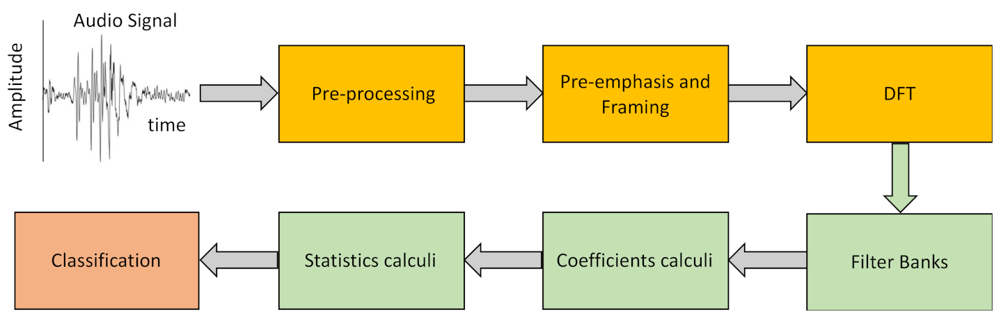
2.4. Laughter Processing
- Pre-Emphasis.The objective of this step is to compensate for the filtering effects exerted by the glottis and the vocal tract on the signal by enhancing the value of the higher frequencies. For this, a high-pass FIR filter (1) is applied to the original signal
- Framing–Windowing.To process an acoustic signal that is continuously changing with time, the original signal is divided into very short segments in which we can assume that its characteristics are static. Further, we employ window overlapping to avoid large variations between the segments to be analyzed, this overlap being less than the size of the selected windows. In a preliminary analysis we have shown that laugh signals can be considered invariant in intervals of duration less than 30 ms. For our study we have used 25 ms-long windows with 10 ms inter-window overlap.
- Discrete Fourier Transform (DFT).After framing, the power spectrum of each window is calculated using Equation (2).
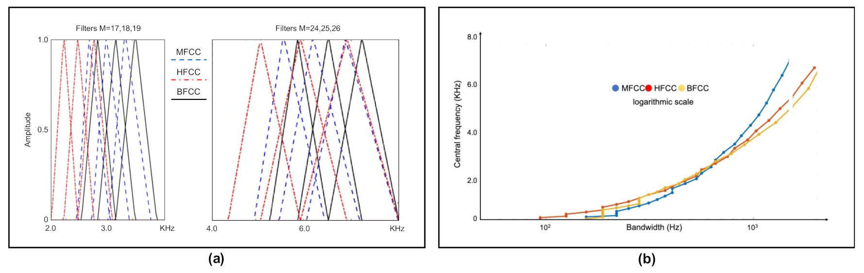
- Filter banks.We have used different filter banks, one for each type of cepstral coefficients. In the case of Mel scale filters, the scale of the power spectrum is transformed into a non-linear scale (Mel scale). For this, the power spectrum is multiplied with the Mel scale filter bank. This transformation is given by Equation (3).
- Laugh characterization.With the above procedure we obtain 13 cepstral coefficients for each of the T frames we divide each laugh into, with T being a high number that depends on the duration of the record. To characterize the laugh, we calculate the mean (μi) and the standard deviation of the mean (SDi) of each of the 13 coefficients for the whole record (i = 1 to 13). However, cepstral coefficients only represent static characteristics of the signal since the T frames of the signal are assumed to be static. To include dynamic information, we additionally calculate Δc and ΔΔc, the first- and second-order variations of the extracted coefficients for each of the T frames using Equations (7) and (8) [36].

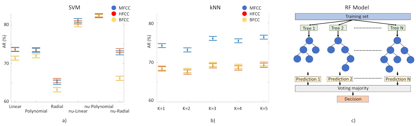
- Laughter classification using automatic classification techniques.For the identification of PD laughs for our decision support system, we have tested the performance of three supervised learning-based classification techniques: (1) Random Forest (RF) model based on the generation of T decision random trees [37]. We execute it 100 times, without pruning. (2) Classification method, kNN [38]. Input elements are represented as vectors and for each one of them the Euclidean distance with each of its k closest neighbors is calculated. Here we tested k = 1 to 10. (3) Support Vector Machine (SVM) [39]. This separates the two classes to be predicted by means of a hyperplane. In this case, we have used a linear kernel, based on previous studies in which this method has been used with MFCC coefficients with successful results. We have used ν-SVC [40] as the SVM type, in such a way that there is a margin of error, upper bound and lower bound, between the examples that may fall into the opposite plane in training: this value has been set at 0.5. Several kernels have been tested: linear, polynomial 3rd degree, radial basis, ν-linear, ν-polynomial 3rd degree, ν-radial basis (Figure 4, left). The 156 component-long characteristic vectors of the laughs were employed as input vectors for these classification methods using the function implemented in WEKA [41]. Models need to be trained to tune up their parameters and then to be validated for the evaluation of their performance. For training and validation, we used subject-wise k-fold cross-validation. This method is based on splitting the dataset in k segments; at every iteration, k-1 segments are used for training and one for validation (Figure 4, right).
- Overall performance of cepstral coefficients.The performance of the three different types of cepstral coefficients in the machine learning models was evaluated according to the accuracy rate (AR), validated through the Mathews correlation coefficient (MCC). Overall performance of the laugh identification-and-classification procedure, expressed by the AR, which represents the percentage of correct predictions given by Equation (9):
- We validated AR results through the Mathews correlation coefficient (MCC), a very good measure method employed in machine learning techniques [1]. MCC is the Pearson’s (or Yule’s) φ coefficient which measures the accuracy of a binary classification [42]. It is calculated from the confusion matrix, and it takes values between 0 and 1, with 0 a random prediction and 1 a perfect prediction [43]. MCC results are in agreement with AR results: the highest score was obtained by RF fed with MFCC, MCC = 0.66 and in the second place we find the SVM fed with HFCC, MCC = 0.64.
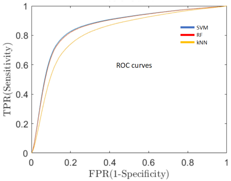
- Sensitivity of the classification algorithms.A good overall performance, a high AR, is a necessary but not sufficient condition for the development of a clinically useful decision support system. One of the fundamental requirements is to minimize the percentage of false negative predictions (ill persons classified as healthy), thus, reducing the number of PD patients that could not be detected and, consequently, would not receive early medical care. For this reason, in addition to AR, we evaluated the sensitivity of the system, which means the capacity of the system to classify true PD patients as having PD, by means of the receiver operating characteristics curve (ROC, Figure 5). ROC is a probability curvethat relates the true positive rate (TPR), i.e., PD subjects correctly classified as PD patients, with the false positive rate (FPR), i.e., healthy subjects erroneously classified as PD ones, at various threshold settings. One of the most important metrics of the ROC curve is the area under the curve (AUC) that measures the degree of separability between the two classes (healthy and PD) [44].
3. Results
4. Discussion
5. Conclusions
Author Contributions
Funding
Institutional Review Board Statement
Informed Consent Statement
Data Availability Statement
Conflicts of Interest
References
- Schneider, F.; Habel, U.; Volkmann, J.; Regel, S.; Kornischka, J.; Sturm, V.; Freund, H.-J. Deep Brain Stimulation of the Subthalamic Nucleus Enhances Emotional Processing in Parkinson Disease. Arch. Gen. Psychiatry 2003, 60, 296–302. [Google Scholar] [CrossRef] [PubMed]
- Svensson, P.; Henningson, C.; Karlsson, S. Speech Motor Control in Parkinson’s Disease: A Comparison between a Clinical Assessment Protocol and a Quantitative Analysis of Mandibular Movements. Folia Phoniatr. Et Logop. 1993, 45, 157–164. [Google Scholar] [CrossRef] [PubMed]
- Draoui, A.; El Hiba, O.; Aimrane, A.; El Khiat, A.; Gamrani, H. Parkinson’s disease: From bench to bedside. Rev. Neurol. 2020, 176, 543–559. [Google Scholar] [CrossRef]
- Joshi, R.; Bronstein, J.M.; Keener, A.; Alcazar, J.; Yang, D.D.; Joshi, M.; Hermanowicz, N. PKG Movement Recording System Use Shows Promise in Routine Clinical Care of Patients with Parkinson’s Disease. Front. Neurol. 2019, 10, 1027. [Google Scholar] [CrossRef] [PubMed]
- Erb, K.; Daneault, J.; Amato, S.; Bergethon, P.; Demanuele, C.; Kangarloo, T.; Patel, S.; Ramos, V.; Volfson, D.; Wacnik, P.; et al. The BlueSky Project: Monitoring motor and non-motor characteristics of people with Parkinson’s disease in the laboratory, a simulated apartment, and home and community settings. Mov. Disord. 2018, 33, 2018. [Google Scholar]
- Rodriguez-Oroz, M.C.; Jahanshahi, M.; Krack, P.; Litvan, I.; Macias, R.; Bezard, E.; Obeso, J.A. Initial clinical manifestations of Parkinson’s disease: Features and pathophysiological mechanisms. Lancet Neurol. 2009, 8, 1128–1139. [Google Scholar] [CrossRef]
- Tjaden, K. Speech and Swallowing in PD. Top Geriatr. Rehabil. 2008, 24, 115–126. [Google Scholar] [CrossRef]
- Skodda, S.; Visser, W.; Schlegel, U. Vowel Articulation in Parkinson’s Disease. J. Voice 2011, 25, 467–472. [Google Scholar] [CrossRef]
- Bang, Y.-I.; Min, K.; Sohn, Y.H.; Cho, S.-R. Acoustic characteristics of vowel sounds in patients with Parkinson disease. NeuroRehabilitation 2013, 32, 649–654. [Google Scholar] [CrossRef]
- Jiménez-Jiménez, F.J.; Gamboa, J.; Nieto, A.; Guerrero, J.; Orti-Pareja, M.; Molina, J.A.; García-Albea, E.; Cobeta, I. Acoustic voice analysis in untreated patients with Parkinson’s disease. Park. Relat. Disord. 1997, 3, 111–116. [Google Scholar] [CrossRef]
- Harel, B.; Cannizzaro, M.; Snyder, P.J. Variability in fundamental frequency during speech in prodromal and incipient Parkinson’s disease: A longitudinal case study. Brain Cogn. 2004, 56, 24–29. [Google Scholar] [CrossRef] [PubMed]
- Rusz, J.; Cmejla, R.; Tykalova, T.; Ruzickova, H.; Klempir, J.; Majerova, V.; Picmausova, J.; Roth, J.; Ruzicka, E. Imprecise vowel articulation as a potential early marker of Parkinson’s disease: Effect of speaking task. J. Acoust. Soc. Am. 2013, 134, 2171–2181. [Google Scholar] [CrossRef] [PubMed]
- Jannetts, S.; Lowit, A. Cepstral Analysis of Hypokinetic and Ataxic Voices: Correlations with Perceptual and Other Acoustic Measures. J. Voice 2014, 28, 673–680. [Google Scholar] [CrossRef] [PubMed]
- Hinton, G.; Deng, L.; Yu, D.; Dahl, G.E.; Mohamed, A.-R.; Jaitly, N.; Senior, A.; Vanhoucke, V.; Nguyen, P.; Sainath, T.N.; et al. Deep Neural Networks for Acoustic Modeling in Speech Recognition: The Shared Views of Four Research Groups. IEEE Signal Process. Mag. 2012, 29, 82–97. [Google Scholar] [CrossRef]
- Tirumala, S.S.; Shahamiri, S.R. A review on Deep Learning approaches in Speaker Identification. In ACM International Conference Proceeding Series; Association for Computing Machinery: New York, NY, USA, 2016; pp. 142–147. [Google Scholar] [CrossRef]
- Marijuán, P.C.; Navarro, J. The bonds of laughter: A multidisciplinary inquiry into the information processes of human laughter. arXiv 2011. arXiv:1010.5602.
- Navarro, J.; Rosell, M.F.; Castellanos, A.; del Moral, R.; Lahoz-Beltra, R.; Marijuán, P.C. Plausibility of a Neural Network Classifier-Based Neuroprosthesis for Depression Detection via Laughter Records. Front. Neurosci. 2019, 13, 267. [Google Scholar] [CrossRef]
- Falkenberg, I.; Klügel, K.; Bartels, M.; Wild, B. Sense of humor in patients with schizophrenia. Schizophr. Res. 2007, 95, 259–261. [Google Scholar] [CrossRef]
- Uekermann, J.; Channon, S.; Lehmkämper, C.; Abdel-Hamid, M.; Vollmoeller, W.; Daum, I. Executive function, mentalizing and humor in major depression. J. Int. Neuropsychol. Soc. 2007, 14, 55–62. [Google Scholar] [CrossRef]
- Giampietri, L.; Belli, E.; Beatino, M.F.; Giannoni, S.; Palermo, G.; Campese, N.; Tognoni, G.; Siciliano, G.; Ceravolo, R.; De Luca, C.; et al. Fluid Biomarkers in Alzheimer’s Disease and Other Neurodegenerative Disorders: Toward Integrative Diagnostic Frameworks and Tailored Treatments. Diagnostics 2022, 12, 796. [Google Scholar] [CrossRef]
- Provine, R.R.; Emmorey, K. Laughter Among Deaf Signers. J. Deaf Stud. Deaf Educ. 2006, 11, 403–409. [Google Scholar] [CrossRef]
- Provine, R.R. Laughing, Tickling, and the Evolution of Speech and Self. Curr. Dir. Psychol. Sci. 2004, 13, 215–218. [Google Scholar] [CrossRef]
- Upadhya, S.S.; Cheeran, A.N.; Nirmal, J.H. Discriminating Parkinson diseased and healthy people using modified MFCC filter bank approach. Int. J. Speech Technol. 2019, 22, 1021–1029. [Google Scholar] [CrossRef]
- Benba, A.; Jilbab, A.; Hammouch, A. Detecting Patients with Parkin son’s disease using Mel Frequency Cepstral Coefficients a nd Support Vector Machines. Int. J. Electr. Eng. Informatics 2015, 7, 297–307. [Google Scholar] [CrossRef]
- Soumaya, Z.; Taoufiq, B.D.; Nsiri, B.; Abdelkrim, A. Diagnosis of Parkinson disease using the wavelet transform and MFCC and SVM classifier. In Proceedings of the 2019 4th World Conference on Complex Systems (WCCS), Ouarzazate, Morocco, 22–25 April 2019; pp. 1–6. [Google Scholar] [CrossRef]
- Navarro, J.; del Moral, R.; Alonso-Sánchez, M.F.; Loste, P.; Garcia-Campayo, J.; Lahoz-Beltra, R.; Marijuán, P. Validation of laughter for diagnosis and evaluation of depression. J. Affect. Disord. 2014, 160, 43–49. [Google Scholar] [CrossRef]
- Audacity® Software; Audacity® software is copyright © 1999–2021 Audacity Team; Morgan Kaufmann Publ. Inc.: Burlington, MA, USA, 2020.
- Gelb, D.J.; Oliver, E.; Gilman, S. Diagnostic Criteria for Parkinson Disease. Arch. Neurol. 1999, 56, 33–39. [Google Scholar] [CrossRef] [PubMed]
- Hoehn, M.M.; Yahr, M.D. Parkinsonism: Onset, progression and mortality. Neurology 1967, 17, 427–442. [Google Scholar] [CrossRef]
- D’haes, W.; Rodet, X. Discrete Cepstrum Coefficients as Perceptual Features. Proc. ICMC. 2003. to be Publ. Available online: http://articles.ircam.fr/textes/Dhaes03b/index.pdf (accessed on 15 August 2022).
- Alim, S.A.; Rashid, N.K.A. Some Commonly Used Speech Feature Extraction Algorithms. In From Natural to Artificial Intelligence—Algorithms and Applications; Intechopen: London, UK, 2018. [Google Scholar]
- Milner, B.; Shao, X. Speech reconstruction from mel-frequency cepstral coefficients using a source-filter model. In Proceedings of the 7th International Conference on Spoken Language Processing (ICSLP 2002), Denver, Colorado, 16–20 September 2002; pp. 2421–2424. [Google Scholar] [CrossRef]
- Davis, S.B.; Mermelstein, P. Comparison of Parametric Representations for Monosyllabic Word Recognition in Continuously Spoken Sentences. Read. Speech Recognit. 1990, 65–74. [Google Scholar] [CrossRef]
- Huang, X.; Acero, A.; Hon, H.-W. Spoken Language Processing: A Guide to Theory, Algorithm & System Development; Prentice-Hall Inc.: Upper Saddle River, NJ, USA, 2001. [Google Scholar]
- MATLAB, version 9.8.0 (R2020a); The MathWorks Inc.: Natick, MA, USA, 2020.
- Muda, L.; Begam, M.; Elamvazuthi, I. Voice Recognition Algorithms using Mel Frequency Cepstral Coefficient (MFCC) and Dynamic Time Warping (DTW) Techniques. J. Comp. 2010, 2, 138–143. [Google Scholar]
- Breiman, L. Random forests. Mach. Learn. 2001, 45, 5–32. [Google Scholar] [CrossRef]
- Silverman, B.W.; Jones, M.C.; Fix, E.; Hodges, J.L. An Important Contribution to Nonparametric Discriminant Analysis and Density Estimation: Commentary on Fix and Hodges (1951). Int. Stat. Rev. 1989, 57, 233. [Google Scholar] [CrossRef]
- Cortes, C.; Vapnik, V. Support-vector networks. Mach. Learn. 1995, 20, 273–297. [Google Scholar] [CrossRef]
- Schölkopf, B.; Smola, A.J.; Williamson, R.C.; Bartlett, P.L. New Support Vector Algorithms. Neural Comput. 2000, 12, 1207–1245. [Google Scholar] [CrossRef] [PubMed]
- Frank, E.; Hall, M.A.; Ian; Witten, H. The WEKA Workbench. Online Appendix for “Data Mining: Practical Machine Learning Tools and Techniques” Morgan Kaufmann, 4th ed.; Morgan Kaufmann Publishers: Burlington, MA, USA, 2016. [Google Scholar]
- Yule, G.U. On the Methods of Measuring Association Between Two Attributes. J. R. Stat. Soc. 1912, 75, 579. [Google Scholar] [CrossRef]
- Stehman, S.V. Selecting and interpreting measures of thematic classification accuracy. Remote Sens. Environ. 1997, 62, 77–89. [Google Scholar] [CrossRef]
- Hanley, J.A.; McNeil, B.J. The meaning and use of the area under a receiver operating characteristic (ROC) curve. Radiology 1982, 143, 29–36. [Google Scholar] [CrossRef] [PubMed]
- Jürgens, U. Neural pathways underlying vocal control. Neurosci. Biobehav. Rev. 2001, 26, 235–258. [Google Scholar] [CrossRef]
- Zarate, J.M. The neural control of singing. Front. Hum. Neurosci. 2013, 7, 237. [Google Scholar] [CrossRef] [Green Version]


| Filter Nr | Mel (MFCC) | Human Factor (HFCC) | Bark (BFCC) |
|---|---|---|---|
| 1 | 62.50 | 31.25 | 62.50 |
| 2 | 156.25 | 125.00 | 156.25 |
| 3 | 218.75 | 187.50 | 218.75 |
| 4 | 312.50 | 281.25 | 312.50 |
| 5 | 406.25 | 375.00 | 375.00 |
| 6 | 531.25 | 468.75 | 468.75 |
| 7 | 656.25 | 593.75 | 562.50 |
| 8 | 781.25 | 718.75 | 656.25 |
| 9 | 937.50 | 843.75 | 750.00 |
| 10 | 1093.75 | 1000.00 | 875.00 |
| 11 | 1250.00 | 1156.25 | 1000.00 |
| 12 | 1437.50 | 1343.75 | 1156.25 |
| 13 | 1656.25 | 1531.25 | 1281.25 |
| 14 | 1875.00 | 1781.25 | 1468.75 |
| 15 | 2125.00 | 2000.00 | 1656.25 |
| 16 | 2406.25 | 2281.25 | 1843.75 |
| 17 | 2718.75 | 2562.50 | 2093.75 |
| 18 | 3062.50 | 2875.00 | 2343.75 |
| 19 | 3437.50 | 3250.00 | 2656.25 |
| 20 | 3812.50 | 3625.00 | 3000.00 |
| 21 | 4281.25 | 4031.25 | 3406.25 |
| 22 | 4750.00 | 4500.00 | 3875.00 |
| 23 | 5281.25 | 5031.25 | 4406.25 |
| 24 | 5875.00 | 5537.50 | 5093.75 |
| 25 | 6531.25 | 6187.50 | 5937.50 |
| 26 | 7218.75 | 6875.00 | 6906.25 |
| Results by employing μ, STD, skewness and kurtosis of the coefficients | ||||||||
|---|---|---|---|---|---|---|---|---|
| Inputs | AR (%) | TP | FP | TN | FN | Sens | Spec | AUC |
| μ(MFCC) | 72 | 0.72 | 0.28 | 0.68 | 0.32 | 0.69 | 0.71 | 0.722 |
| STD(MFCC) | 68 | 0.67 | 0.33 | 0.69 | 0.31 | 0.68 | 0.67 | 0.695 |
| skew(MFCC) | 59 | 0.58 | 0.42 | 0.61 | 0.39 | 0.6 | 0.59 | 0.615 |
| kurt(MFCC) | 60 | 0.62 | 0.38 | 0.59 | 0.41 | 0.6 | 0.61 | 0.625 |
| μ(HFCC) | 72 | 0.72 | 0.28 | 0.69 | 0.32 | 0.7 | 0.71 | 0.725 |
| STD(HFCC) | 70 | 0.7 | 0.3 | 0.69 | 0.31 | 0.7 | 0.7 | 0.721 |
| skew(HFCC) | 65 | 0.65 | 0.35 | 0.65 | 0.35 | 0.65 | 0.65 | 0.67 |
| kurt(HFCC) | 70 | 0.71 | 0.29 | 0.68 | 0.32 | 0.69 | 0.7 | 0.715 |
| μ(BFCC) | 73 | 0.72 | 0.28 | 0.7 | 0.3 | 0.71 | 0.71 | 0.733 |
| STD(BFCC) | 70 | 0.7 | 0.3 | 0.69 | 0.31 | 0.69 | 0.69 | 0.712 |
| skew(BFCC) | 57 | 0.57 | 0.43 | 0.58 | 0.42 | 0.57 | 0.57 | 0.599 |
| kurt(BFCC) | 63 | 0.65 | 0.35 | 0.62 | 0.39 | 0.63 | 0.63 | 0.654 |
| Results by employing μ, STD, skewness and kurtosis of the delta (Δ) of the coefficients | ||||||||
| Inputs | AR (%) | TP | FP | TN | FN | Sens | Spec | AUC |
| μ(Δ(MFCC)) | 67 | 0.69 | 0.31 | 0.65 | 0.35 | 0.66 | 0.68 | 0.692 |
| STD(Δ(MFCC)) | 74 | 0.7 | 0.3 | 0.65 | 0.35 | 0.66 | 0.68 | 0.694 |
| skew(Δ(MFCC)) | 64 | 0.65 | 0.35 | 0.64 | 0.36 | 0.64 | 0.65 | 0.665 |
| kurt(Δ(MFCC)) | 62 | 0.64 | 0.36 | 0.6 | 0.4 | 0.62 | 0.63 | 0.645 |
| μ(Δ(HFCC)) | 69 | 0.7 | 0.3 | 0.68 | 0.32 | 0.69 | 0.69 | 0.712 |
| STD(Δ(HFCC)) | 70 | 0.68 | 0.32 | 0.67 | 0.33 | 0.67 | 0.68 | 0.695 |
| skew(Δ(HFCC)) | 70 | 0.7 | 0.3 | 0.71 | 0.29 | 0.7 | 0.7 | 0.72 |
| kurt(Δ(HFCC)) | 64 | 0.67 | 0.33 | 0.61 | 0.39 | 0.63 | 0.65 | 0.664 |
| μ(Δ(BFCC)) | 63 | 0.65 | 0.35 | 0.62 | 0.38 | 0.63 | 0.64 | 0.657 |
| STD(Δ(BFCC)) | 71 | 0.68 | 0.32 | 0.69 | 0.31 | 0.69 | 0.69 | 0.71 |
| skew(Δ(BFCC)) | 68 | 0.69 | 0.31 | 0.67 | 0.33 | 0.68 | 0.68 | 0.701 |
| kurt(Δ(BFCC)) | 63 | 0.66 | 0.35 | 0.6 | 0.4 | 0.62 | 0.64 | 0.656 |
| Results by employing μ, STD, skewness and kurtosis of the delta-delta (ΔΔ) of the coefficients | ||||||||
| Inputs | AR (%) | TP | FP | TN | FN | Sens | Spec | AUC |
| μ(ΔΔ(MFCC)) | 69 | 0.72 | 0.28 | 0.65 | 0.35 | 0.68 | 0.7 | 0.712 |
| STD(ΔΔ(MFCC)) | 71 | 0.78 | 0.22 | 0.75 | 0.25 | 0.71 | 0.72 | 0.735 |
| skew(ΔΔ(MFCC)) | 61 | 0.8 | 0.2 | 0.77 | 0.23 | 0.61 | 0.61 | 0.634 |
| kurt(ΔΔ(MFCC)) | 66 | 0.79 | 0.21 | 0.77 | 0.23 | 0.66 | 0.66 | 0.685 |
| μ(ΔΔ(HFCC)) | 69 | 0.71 | 0.29 | 0.66 | 0.34 | 0.68 | 0.7 | 0.713 |
| STD(ΔΔ(HFCC)) | 71 | 0.73 | 0.27 | 0.69 | 0.31 | 0.7 | 0.72 | 0.734 |
| skew(ΔΔ(HFCC)) | 66 | 0.65 | 0.35 | 0.66 | 0.34 | 0.66 | 0.65 | 0.675 |
| kurt(ΔΔ(HFCC)) | 61 | 0.63 | 0.37 | 0.6 | 0.4 | 0.61 | 0.62 | 0.635 |
| μ(ΔΔ(BFCC)) | 63 | 0.65 | 0.35 | 0.62 | 0.38 | 0.63 | 0.64 | 0.655 |
| STD(ΔΔ(BFCC)) | 73 | 0.74 | 0.26 | 0.73 | 0.27 | 0.73 | 0.73 | 0.754 |
| skew(ΔΔ(BFCC)) | 70 | 0.7 | 0.3 | 0.69 | 0.31 | 0.69 | 0.7 | 0.715 |
| kurt(ΔΔ(BFCC)) | 60 | 0.58 | 0.42 | 0.62 | 0.38 | 0.6 | 0.6 | 0.626 |
| Results by employing μ, STD, skewness and kurtosis of the coefficients | ||||||||
|---|---|---|---|---|---|---|---|---|
| Inputs | AR (%) | TP | FP | TN | FN | Sens | Spec | AUC |
| μ(MFCC) | 72 | 0.72 | 0.28 | 0.68 | 0.32 | 0.69 | 0.71 | 0.71 |
| μ+STD(MFCC) | 74 | 0.75 | 0.25 | 0.73 | 0.27 | 0.73 | 0.74 | 0.75 |
| μ+STD+skew(MFCC) | 75 | 0.76 | 0.24 | 0.74 | 0.26 | 0.74 | 0.75 | 0.76 |
| μ+STD+skew+kurt(MFCC) | 76 | 0.77 | 0.23 | 0.76 | 0.24 | 0.76 | 0.77 | 0.78 |
| μ(HFCC) | 72 | 0.72 | 0.28 | 0.69 | 0.31 | 0.70 | 0.71 | 0.72 |
| μ+STD(HFCC) | 74 | 0.74 | 0.26 | 0.73 | 0.27 | 0.74 | 0.74 | 0.76 |
| μ+STD+skew(HFCC) | 76 | 0.77 | 0.23 | 0.75 | 0.25 | 0.76 | 0.76 | 0.78 |
| μ+STD+skew+kurt(HFCC) | 77 | 0.79 | 0.21 | 0.76 | 0.24 | 0.77 | 0.78 | 0.80 |
| μ(BFCC) | 73 | 0.72 | 0.28 | 0.70 | 0.30 | 0.71 | 0.71 | 0.73 |
| μ+STD(BFCC) | 74 | 0.75 | 0.25 | 0.73 | 0.27 | 0.73 | 0.74 | 0.76 |
| μ+STD+skew(BFCC) | 75 | 0.76 | 0.24 | 0.74 | 0.26 | 0.75 | 0.75 | 0.77 |
| μ+STD+skew+kurt(BFCC) | 76 | 0.77 | 0.23 | 0.75 | 0.25 | 0.76 | 0.76 | 0.79 |
| Results by employing μ, STD, skewness and kurtosis of the delta (Δ) of the coefficients | ||||||||
| Inputs | AR (%) | TP | FP | TN | FN | Sens | Spec | AUC |
| μ(Δ(MFCC)) | 67 | 0.69 | 0.31 | 0.65 | 0.35 | 0.66 | 0.68 | 0.69 |
| μ+STD(Δ(MFCC)) | 72 | 0.73 | 0.27 | 0.72 | 0.28 | 0.72 | 0.73 | 0.75 |
| μ+STD+skew(Δ(MFCC)) | 73 | 0.75 | 0.25 | 0.72 | 0.28 | 0.73 | 0.74 | 0.76 |
| μ+STD+skew+kurt(Δ(MFCC)) | 75 | 0.76 | 0.24 | 0.75 | 0.25 | 0.75 | 0.76 | 0.78 |
| μ(Δ(HFCC)) | 69 | 0.7 | 0.3 | 0.68 | 0.32 | 0.69 | 0.69 | 0.71 |
| μ+STD(Δ(HFCC)) | 72 | 0.71 | 0.29 | 0.72 | 0.28 | 0.72 | 0.71 | 0.74 |
| μ+STD+skew(Δ(HFCC)) | 73 | 0.73 | 0.27 | 0.73 | 0.27 | 0.73 | 0.73 | 0.75 |
| μ+STD+skew+kurt(Δ(HFCC)) | 76 | 0.76 | 0.24 | 0.76 | 0.24 | 0.76 | 0.76 | 0.78 |
| μ(Δ(BFCC)) | 63 | 0.65 | 0.35 | 0.62 | 0.38 | 0.63 | 0.64 | 0.66 |
| μ+STD(Δ(BFCC)) | 67 | 0.67 | 0.33 | 0.68 | 0.32 | 0.67 | 0.67 | 0.69 |
| μ+STD+skew(Δ(BFCC)) | 69 | 0.69 | 0.31 | 0.70 | 0.30 | 0.69 | 0.69 | 0.71 |
| μ+STD+skew+kurt(Δ(BFCC)) | 71 | 0.72 | 0.28 | 0.72 | 0.28 | 0.72 | 0.72 | 0.74 |
| Results by employing μ, STD, skewness and kurtosis of the delta-delta (ΔΔ) of the coefficients | ||||||||
| Inputs | AR (%) | TP | FP | TN | FN | Sens | Spec | AUC |
| μ(ΔΔ(MFCC)) | 69 | 0.72 | 0.28 | 0.65 | 0.35 | 0.68 | 0.70 | 0.71 |
| μ+STD(ΔΔ(MFCC)) | 76 | 0.78 | 0.22 | 0.75 | 0.25 | 0.76 | 0.77 | 0.79 |
| μ+STD+skew(ΔΔ(MFCC)) | 78 | 0.79 | 0.21 | 0.77 | 0.23 | 0.78 | 0.79 | 0.81 |
| μ+STD+skew+kurt(ΔΔ(MFCC)) | 78 | 0.80 | 0.20 | 0.77 | 0.23 | 0.78 | 0.79 | 0.81 |
| μ(ΔΔ(HFCC)) | 69 | 0.71 | 0.29 | 0.66 | 0.34 | 0.68 | 0.70 | 0.71 |
| μ+STD(ΔΔ(HFCC)) | 75 | 0.76 | 0.24 | 0.73 | 0.27 | 0.74 | 0.75 | 0.77 |
| μ+STD+skew(ΔΔ(HFCC)) | 75 | 0.77 | 0.24 | 0.74 | 0.26 | 0.75 | 0.76 | 0.78 |
| μ+STD+skew+kurt(ΔΔ(HFCC)) | 76 | 0.77 | 0.23 | 0.75 | 0.25 | 0.75 | 0.77 | 0.78 |
| μ(ΔΔ(BFCC)) | 63 | 0.65 | 0.35 | 0.62 | 0.38 | 0.63 | 0.64 | 0.66 |
| μ+STD(ΔΔ(BFCC)) | 72 | 0.73 | 0.27 | 0.72 | 0.28 | 0.72 | 0.72 | 0.74 |
| μ+STD+skew(ΔΔ(BFCC)) | 73 | 0.73 | 0.27 | 0.73 | 0.27 | 0.73 | 0.73 | 0.75 |
| μ+STD+skew+kurt(ΔΔ(BFCC)) | 74 | 0.75 | 0.26 | 0.74 | 0.26 | 0.74 | 0.74 | 0.76 |
| Inputs | AR (%) | TP | FP | TN | FN | Sens | Spec | AUC |
|---|---|---|---|---|---|---|---|---|
| μ(MFCC+Δ(MFCC)+ΔΔ(MFCC)) | 74 | 0.77 | 0.23 | 0.71 | 0.29 | 0.73 | 0.76 | 0.75 |
| μ+STD(MFCC+Δ(MFCC)+ΔΔ(MFCC)) | 82 | 0.83 | 0.17 | 0.82 | 0.18 | 0.82 | 0.83 | 0.84 |
| μ+STD+skew(MFCC+Δ(MFCC)+ΔΔ(MFCC)) | 83 | 0.84 | 0.16 | 0.82 | 0.18 | 0.82 | 0.84 | 0.85 |
| μ+STD+skew+kurt(MFCC+Δ(MFCC)+ΔΔ(MFCC)) | 83 | 0.84 | 0.16 | 0.82 | 0.18 | 0.83 | 0.84 | 0.86 |
| μ(HFCC+Δ(HFCC)+ΔΔ(HFCC)) | 75 | 0.77 | 0.23 | 0.73 | 0.27 | 0.74 | 0.76 | 0.76 |
| μ+STD(HFCC+Δ(HFCC)+ΔΔ(HFCC)) | 81 | 0.82 | 0.18 | 0.81 | 0.19 | 0.81 | 0.82 | 0.83 |
| μ+STD+skew(HFCC+Δ(HFCC)+ΔΔ(HFCC)) | 82 | 0.83 | 0.17 | 0.82 | 0.18 | 0.82 | 0.82 | 0.84 |
| μ+STD+skew+kurt(HFCC+Δ(HFCC)+ΔΔ(HFCC)) | 82 | 0.83 | 0.17 | 0.82 | 0.18 | 0.82 | 0.83 | 0.85 |
| μ(BFCC+Δ(BFCC)+ΔΔ(BFCC)) | 72 | 0.74 | 0.26 | 0.70 | 0.30 | 0.74 | 0.71 | 0.76 |
| μ+STD(BFCC+Δ(BFCC)+ΔΔ(BFCC)) | 80 | 0.80 | 0.20 | 0.80 | 0.20 | 0.80 | 0.80 | 0.82 |
| μ+STD+skew(BFCC+Δ(BFCC)+ΔΔ(BFCC)) | 81 | 0.81 | 0.19 | 0.81 | 0.19 | 0.81 | 0.81 | 0.84 |
| μ+STD+skew+kurt(BFCC+Δ(BFCC)+ΔΔ(BFCC)) | 82 | 0.82 | 0.18 | 0.81 | 0.19 | 0.82 | 0.81 | 0.85 |
| Results of Mel filters: μ + STD + skew + kurt (MFCC + Δ(MFCC) + ΔΔ(MFCC)) | ||||||||
|---|---|---|---|---|---|---|---|---|
| Kernel variation | AR (%) | TP | FP | TN | FN | Sens | Spec | AUC |
| Linear | 74 | 0.74 | 0.26 | 0.73 | 0.27 | 0.73 | 0.74 | 0.76 |
| Polynomial | 73 | 0.75 | 0.25 | 0.72 | 0.28 | 0.73 | 0.74 | 0.76 |
| Radial Basis | 65 | 0.86 | 0.14 | 0.45 | 0.55 | 0.61 | 0.76 | 0.72 |
| ν-Linear | 81 | 0.81 | 0.19 | 0.81 | 0.19 | 0.81 | 0.81 | 0.85 |
| ν-Polynomial | 82 | 0.82 | 0.18 | 0.83 | 0.17 | 0.82 | 0.82 | 0.86 |
| ν-Radial Basis | 73 | 0.85 | 0.15 | 0.60 | 0.40 | 0.68 | 0.80 | 0.79 |
| Results of Human Factor filters: μ + STD + skew + kurt (HFCC + Δ(HFCC) + ΔΔ(HFCC)) | ||||||||
| Kernel variation | AR (%) | TP | FP | TN | FN | Sens | Spec | AUC |
| Linear | 74 | 0.74 | 0.26 | 0.73 | 0.27 | 0.74 | 0.74 | 0.78 |
| Polynomial | 74 | 0.75 | 0.25 | 0.73 | 0.27 | 0.73 | 0.74 | 0.78 |
| Radial Basis | 66 | 0.86 | 0.14 | 0.45 | 0.55 | 0.61 | 0.76 | 0.73 |
| ν-Linear | 81 | 0.81 | 0.19 | 0.81 | 0.19 | 0.81 | 0.81 | 0.85 |
| ν-Polynomial | 83 | 0.83 | 0.17 | 0.83 | 0.17 | 0.83 | 0.83 | 0.86 |
| ν-Radial Basis | 73 | 0.85 | 0.15 | 0.61 | 0.39 | 0.69 | 0.81 | 0.79 |
| Results of Bark filters: μ + STD + skew + kurt (BFCC + Δ(BFCC) + ΔΔ(BFCC)) | ||||||||
| Kernel variation | AR (%) | TP | FP | TN | FN | Sens | Spec | AUC |
| Linear | 71 | 0.71 | 0.29 | 0.72 | 0.28 | 0.72 | 0.71 | 0.76 |
| Polynomial | 72 | 0.72 | 0.28 | 0.72 | 0.28 | 0.72 | 0.72 | 0.76 |
| Radial Basis | 63 | 0.85 | 0.15 | 0.41 | 0.59 | 0.59 | 0.73 | 0.69 |
| ν-Linear | 80 | 0.80 | 0.20 | 0.80 | 0.20 | 0.80 | 0.80 | 0.85 |
| ν-Polynomial | 82 | 0.82 | 0.18 | 0.82 | 0.18 | 0.82 | 0.82 | 0.86 |
| ν-Radial Basis | 66 | 0.85 | 0.15 | 0.47 | 0.53 | 0.62 | 0.76 | 0.72 |
| AR (%) | TP | FP | TN | FN | Sens | Spec | AUC | |
|---|---|---|---|---|---|---|---|---|
| MFCC | 83 | 0.84 | 0.16 | 0.82 | 0.18 | 0.83 | 0.84 | 0.86 |
| HFCC | 82 | 0.83 | 0.17 | 0.82 | 0.18 | 0.82 | 0.83 | 0.85 |
| BFCC | 81 | 0.82 | 0.18 | 0.81 | 0.19 | 0.82 | 0.81 | 0.85 |
Publisher’s Note: MDPI stays neutral with regard to jurisdictional claims in published maps and institutional affiliations. |
© 2022 by the authors. Licensee MDPI, Basel, Switzerland. This article is an open access article distributed under the terms and conditions of the Creative Commons Attribution (CC BY) license (https://creativecommons.org/licenses/by/4.0/).
Share and Cite
Terriza, M.; Navarro, J.; Retuerta, I.; Alfageme, N.; San-Segundo, R.; Kontaxakis, G.; Garcia-Martin, E.; Marijuan, P.C.; Panetsos, F. Use of Laughter for the Detection of Parkinson’s Disease: Feasibility Study for Clinical Decision Support Systems, Based on Speech Recognition and Automatic Classification Techniques. Int. J. Environ. Res. Public Health 2022, 19, 10884. https://doi.org/10.3390/ijerph191710884
Terriza M, Navarro J, Retuerta I, Alfageme N, San-Segundo R, Kontaxakis G, Garcia-Martin E, Marijuan PC, Panetsos F. Use of Laughter for the Detection of Parkinson’s Disease: Feasibility Study for Clinical Decision Support Systems, Based on Speech Recognition and Automatic Classification Techniques. International Journal of Environmental Research and Public Health. 2022; 19(17):10884. https://doi.org/10.3390/ijerph191710884
Chicago/Turabian StyleTerriza, Miguel, Jorge Navarro, Irene Retuerta, Nuria Alfageme, Ruben San-Segundo, George Kontaxakis, Elena Garcia-Martin, Pedro C. Marijuan, and Fivos Panetsos. 2022. "Use of Laughter for the Detection of Parkinson’s Disease: Feasibility Study for Clinical Decision Support Systems, Based on Speech Recognition and Automatic Classification Techniques" International Journal of Environmental Research and Public Health 19, no. 17: 10884. https://doi.org/10.3390/ijerph191710884
APA StyleTerriza, M., Navarro, J., Retuerta, I., Alfageme, N., San-Segundo, R., Kontaxakis, G., Garcia-Martin, E., Marijuan, P. C., & Panetsos, F. (2022). Use of Laughter for the Detection of Parkinson’s Disease: Feasibility Study for Clinical Decision Support Systems, Based on Speech Recognition and Automatic Classification Techniques. International Journal of Environmental Research and Public Health, 19(17), 10884. https://doi.org/10.3390/ijerph191710884