1. Introduction
In recent years, the human impact on the global ecology has increased dramatically. Therefore, the importance to control the rate of anthropogenic changes has intensified, inter alia, the need of gathering accurate and timely landcover information. Many remote sensing techniques have been introduced to continuously monitor Earth’s surface in order to obtain useful data for environmental management improvement.
Land cover classification is one of the major topics being investigated in the field of remote sensing [
1]. Advanced technology sensors attached to satellites provide perpetually high-quality information such as hyperspectral images [
2] and InSAR and PolSAR data [
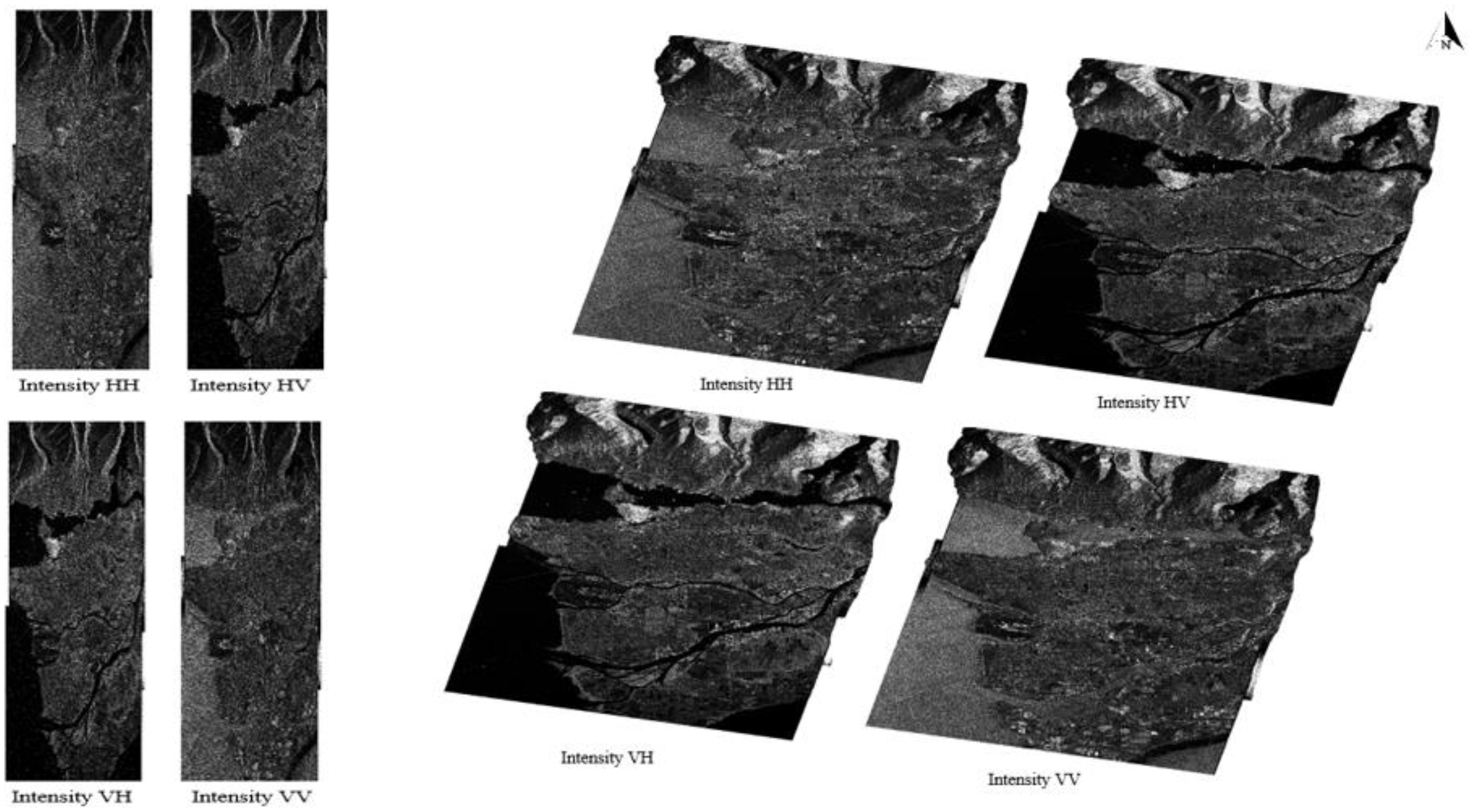
3] which optimize and greatly increase the accuracy of land cover classification procedures. PolSAR is an active radar system that transmits and receives microwaves, providing a desirable capacity for all weather, day and night imaging. In this research, data from fully polarimetric SAR, also known as quad-polarization SAR, are utilized. Quad-pol is a mode of SAR imagery which transmits and receives signals of multiple polarization states (HH, HV, VH, VV), capturing all the polarization information available in the backscattered wave. The acquired data are usually represented in a matrix form. Algorithms known as polarimetric target decomposition techniques have been introduced to obtain features which can describe PolSAR images in multiple aspects in order to be utilized in classification and target detection procedures. In the last decade, several land cover classification techniques have been developed utilizing quad-pol data. Most of them combine features extracted using decomposition techniques with machine learning algorithms, achieving remarkable results. In this work, a new land cover classification scheme is introduced. Specifically, the present research focuses on two novel procedures:
Firstly, the implementation of the new established method for PolSAR data processing known as the Double Scatterer Model is carried out, in order to utilize the primary and secondary scatterers with the contribution rates. Based on these parameters a new PolSAR data form is presented.
Secondly, a fully interconnected neural network is designed for the specific supervised classification task. A pixel window is used to determine the input pixels and assimilate, in this way, data of spatially adjacent pixels in both training and test sets.
It is noteworthy that in this research, the first technique of exploiting the Double Scatterer Model is presented and it is combined with an algorithm specially designed to exploit the greatest possible amount of information to be used in the classification process.
2. Related Works
The first target decomposition method was developed by S. Chandrasekhar [
4] in his work on light scattering by small anisotropic particles. In particular, an analysis of phase matrix into a sum of three independent components was presented. In J.R. Huynens’ PhD dissertation [
5] a decomposition of an average Mueller matrix into the sum of a matrix corresponds to a pure target and an N-target matrix was introduced.
S.R. Cloude [
6] was the first to consider an incoherent target decomposition method based on eigenvector analysis of a coherency matrix, which extracts the dominant scattering mechanism from a PolSAR cell through the calculation of the greater eigenvalue. In the sequel, S.R. Cloude and E. Pottier [
7] proposed the representation of scattering characteristics by the space of entropy
and the averaged scattering angle
. Equivalent information as in the S.R. Cloude and E. Pottier decomposition is extracted in [
8] by utilizing a unique target scattering type parameter which jointly uses the Barakat degree of polarization and the element of the polarimetric coherency matrix.
A model-based decomposition approach has been introduced by A. Freeman and S.L. Durden [
9] which fits a physically based three-component scattering model to the polarimetric SAR data. This technique decomposes the covariance matrix into three categories, surface, volume and even-bounce scattering. One basic assumption of this model is the reflection symmetry, which limits its applicability to only reflection symmetric targets. To overcome this problem, Y. Yamaguchi et al. [
10] proposed a four-component scattering model by introducing an additional term corresponding to non-reflection symmetric targets. Recently, a model-free four-component scattering power decomposition that alleviates the compensations of the parameter of the orientation angle about the radar line of sight and the occurrence of negative power components was introduced in [
11].
Coherent target decompositions analyze the scattering matrix as a weighted combination of scattering response of simple or canonical objects. One of the widely used methods is Pauli spin matrices. Based on both Pauli decomposition and Huynen’s work [
5], W.L. Cameron and L.K. Leung [
12] proposed a stepwise coherent decomposition for the scattering matrix utilizing the properties of reciprocity and symmetry, including a classification scheme.
Lately, K. Karachristos et al. [
13] exploited Cameron’s coherent decomposition to introduce the Double Scatterer Model, a novel method representing PolSAR cells’ information by a pair of elementary scattering mechanisms, each one contributing to the scattering behavior with its own weight. Thus, a new feature-tool was established, well suited for both detection and classification tasks.
In [
14], more than 20 polarimetric decomposition methods were used to extract a set of features which were optimized to improve land cover classification using the object-oriented RF-SFS algorithm. X. Liu et al. [
15] utilized a polarimetric convolutional network for PolSAR image classification, introducing a new encoding method for a scattering matrix with remarkable results. L. Zhang et al. [
16] employed a multiple-component scattering model, Cloude–Pottier decomposition and gray-level co-occurrence matrix to obtain features for PolSAR image description, in order to classify five land cover types based on sparse representation. G. Koukiou and V. Anastassopoulos classified land cover types implementing Markov chains on features extracted by Cameron’s decomposition [
17]. The application of hidden Markov models for a supervised classification combined with Cameron’s scattering technique was carried out by K. Karachristos et al. [
18]. The results of all the above methods confirm the dynamic application of the combination of polarimetric decomposition algorithms and machine learning.
This paper is structured as follows:
Section 3 describes the employed fully polarimetric data and the preprocessing that was used.
Section 4 provides the background on Cameron’s coherent decomposition and introduces the Double Scatterer Model. In
Section 5, a brief review of artificial neural networks is made. Our proposed classification procedure is analyzed in
Section 6 and the results are presented in
Section 7, while the conclusions are drawn in the final
Section 8.
4. Double Scatterer Model
The Double Scatterer Model could be introduced as an extension of Cameron’s coherent decomposition, so that each PolSAR cell is interpreted by a pair of fundamental scattering mechanisms.
In particular, W.L. Cameron and L.K. Leung [
12] presented a technique of decomposing the polarization scattering matrix into three parts, based on the properties of reciprocity and symmetry. The three parts are non-reciprocal, asymmetric and symmetric. According to this separation, 11 classes can arise to characterize the scattering matrix under examination, namely the non-reciprocal, the asymmetric, left and right helix and 7 classes of symmetric elementary scattering mechanisms, 6 of which are known geometrical structures (trihedral, dihedral, dipole, ¼ wave device, cylinder, narrow diplane) and the last one corresponds to a symmetric class with unknown structure.
Cameron’s stepwise algorithm proceeds as follows:
Firstly, the scattering matrix
is expressed on the Pauli basis:
where
Following Cameron’s algorithm, sometimes it is convenient to view the matrix
as a vector
:
The vector
is related to the matrix
by the operators
which are defined as
Thus, leading the expression of
to be:
The hat of vector symbolizes a unit vector ( where stands for vector magnitude).
Secondly, based on the reciprocity theorem, according to which
, Cameron divides the respective target into reciprocal or non-reciprocal. This is carried out by calculating the projection angle of the scattering matrix in the reciprocal subspace:
If the projection angle is less than
, the elementary scattering is considered as reciprocal, otherwise it is taken as non-reciprocal. The scattering matrix of a reciprocal scatterrer is now decomposed as:
Since in (9) the only non-reciprocal component is with the non-diagonal elements to be opposite.
Ultimately, the reciprocal scatterer in a vector form is expressed as follows:
Lastly, Cameron further decomposes the matrix which corresponds to a reciprocal elementary scattering mechanism into a symmetric and an asymmetric component. A scatterer can be identified as symmetric when the target has an axis of symmetry in the plane perpendicular to the radar LOS, or alternatively if there exists a rotation
that cancels out the projection of
on the antisymmetric component
. If such an angle exists, then the symmetric component of the reciprocal scatterer becomes maximum. The rotation angel
corresponds to the scatterer orientation angle. The maximum symmetric component of the reciprocal scatterer is defined as:
with
and
As for the degree of symmetry, it is expressed as the degree to which
deviates from
and it can be calculated as follows:
where
stands for the norm of a complex vector form to which the matrix corresponds. If
, then the scattering matrix corresponds to a perfectly symmetric target. If
, the target that backscatters the radiation is considered asymmetric. Cameron considers as symmetric any elementary scattering with angle
.
Thus, an arbitrary scatterer
that obeys the reciprocity and symmetry theorem as formulated in Cameron’s method can be decomposed according to
where
indicates the amplitude of the scattering matrix,
is the nuisance phase and
is the scatterer orientation angle. The matrix
denotes the rotation operator and
is given by:
with
being referred to as a complex parameter that eventually determines the scattering mechanism.
In
Table 1 are given the complex vectors
and the corresponding values of
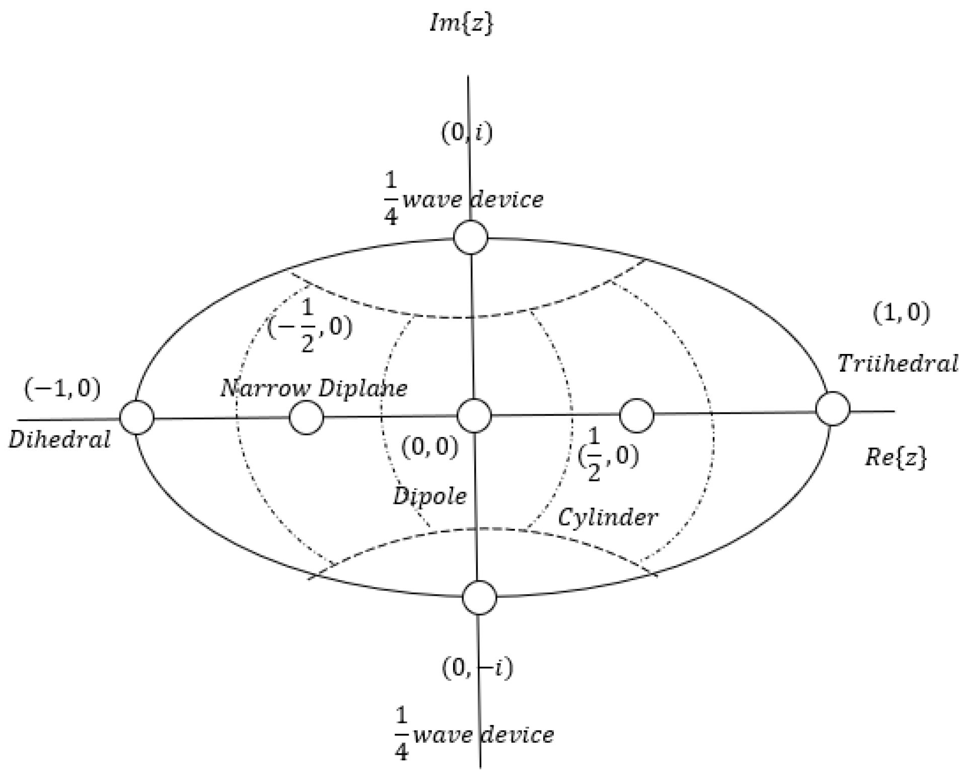
for symmetric elementary scattering mechanisms. The range of the
parameter implies that the scattering matrix can be represented by a point on the unit disk of the complex plane. The positions of the various types of elementary scattering mechanisms are shown on the unit circle represented in
Figure 3 along with the regions on the unit disk which are considered as belonging to these scattering mechanisms. Evidently, and according to the values of
given in
Table 1, all elementary scatterers lie on the diameter of the unit disk except for the ¼ wave devices which lie on the imaginary axis.
In order to determine the scattering behavior of an unknown scattering target
, Cameron considered the following distance metric [
12]:
Cameron et al. [
24] noticed the need for a closed surface rather than the disk, as a result of the double presence of the ¼ wave device. Ideally, the symmetric space could be the unit sphere. This was thoroughly demonstrated by a mapping procedure proposed in [
24]. This mapping procedure is depicted in
Figure 4. Specifically, in the new topology, they associated each point
of the unit disk with a circular arc
on the unit sphere containing the points
,
and
.
Obviously, for the point
not on the rim of the disk, the arc length is less than
. In such a case, the arc would be “stretched” to have length equal to
and be part of a great circle. By associating each point
with a semi-circle, the way this mapping works is easily depicted, by placing these circles tangent on the sphere’s surface with the initial position
of the point on the unit disk determining the latitude
and longitude
of the point on the unit sphere. This mapping is represented in
Figure 4, according to [
24] with spherical coordinates
and
given by:
where
The space distance measure
of a test scatterer
and each of the reference scattering mechanisms of
Table 1 are now given by an equivalent to (20), but more intuitive, form:
with
and
With a view to collect the highest amount of polarimetric information, K. Karachristos et al. [
13] present the Double Scatterer Model, an algorithm-extension of Cameron’s stepwise procedure. Basically, they proposed a method to interpret each PolSAR cell as a contribution of the two most dominant elementary scattering mechanisms in order to extract rich information content. Specifically, the main steps of the method are the following:
For each scattering matrix, the complex parameter will be computed. If the criteria of reciprocity and symmetry are met, the imaginary and the real part of will determine a point on the complex unit disk, according to Cameron’s algorithm.
The mapping of the point on the surface of the unit sphere follows. The PolSAR cell under examination and its scattering matrix are now represented by the longitude
and the latitude
on the unit sphere (
Figure 5).
According to Poelman [
25], the elemental scattering mechanisms of cylinder and narrow diplane can be obtained as a linear combination of the rest of the elementary scatterers:
Since the scattering mechanisms of cylinder and narrow diplane can be composed of trihedral, dipole and dihedral, the three mentioned above as well as the ¼ wave device can be characterized as the fundamental scattering mechanisms. This claim led us to disregard the scattering mechanisms of cylinder and narrow diplane as being of minimum importance and update the spherical topology as depicted in
Figure 5.
- 4.
The location of the right-angled spherical triangle depends on the angle values
of the point under examination. Whether it is above or below the equator, one vertex of the triangle will always be the one pole of the sphere and the other two, the nearest scattering mechanisms calculated by using the orthodromic/great circle distance
:
- 5.
The vector with an initial point on the sphere’s center and the terminal one given by the coordinates on the spherical shell are projected on the level of the equator to which the reference scattering mechanisms belong, based on the angle
(
Figure 5). Specifically, the projection is contained in the quadrant enclosed by the center of the sphere and the two closest to the examination point scatterers.
- 6.
The immediate consequence is the analysis of the projection of the vector in two vertical components which are the two nearest scatterers.
Based on the above, the mixture interpretation for each scatterer is accomplished by:
where
It is important to note the computes the contribution degree of each of the two dominating fundamental scattering mechanisms. When is approaching 1 or 100%, it means that the target scatterer is fully described by one of the four fundamental scattering mechanisms.
In the marginal case where , the scatterer can be assumed as undetermined and be classified as “non-categorizable”. The same class is used for asymmetric scatterers.
5. Artificial Neural Networks (ANNs)
In its most general form, a neural network is a machine that is designed to model the way in which the brain performs a particular task or function of interest. To achieve good performance, neural networks employ a massive interconnection of simple computing cells referred to as “neurons” or processing units. S. Haykin [
26] offers the following definition of a neural network viewed as an adaptive machine:
A neural network is a massively parallel distributed processor made up of simple processing units, which has a natural propensity for storing experiential knowledge and making it available for use. It resembles the brain in two respects:
Knowledge is acquired by the network from its environment through a learning process.
Interneuron connection strengths, known as synaptic weights, are used to store the acquired knowledge.
The procedure used to perform the learning process is called a learning algorithm, the function of which is to modify the synapsis weights of the network in an orderly fashion to action a desired design objective.
The multilayer perceptron (MLP) neural network, a model that uses a single- or multilayer perceptron to approximate the inherent input–output relationships, is the most commonly used network model for image classification in remote sensing [
27,
28]. Typically, the network consists of a set of sensory units (source nodes) that constitute the input layer, one or more hidden layers of computational units and one output layer (
Figure 6). The essential components of MLP are the architecture, involving the numbers of neurons and layers of the network, and the learning algorithm. MLP networks are usually trained with the supervised backpropagation (BP) algorithm [
29]. This algorithm is based on the error-correction learning rule. Basically, error backpropagation learning consists of two passes through the different layers of the network: a forward pass and a backward one. In the forward pass, an activity pattern (input vector) is applied to the sensory nodes of the network and its effect propagates through the network layer by layer. Finally, a set of outputs is produced as the actual response of the network. During the forward pass, the synaptic weights of the network are all fixed. During the backward pass, the synaptic weights are all adjusted in accordance with an error-correction rule. Specifically, the actual response of the network is subtracted from a desired response to produce an error signal. This error signal is then propagated backward through the network, hence the name “error backpropagation”. The synaptic weights are adjusted to make the actual response of the network move closer to the desired response, in a statistical sense. Apart from the architecture of the MLP and the learning algorithm, operational factors such as data characteristics and training parameters can affect the model performance. However, these factors are application-dependent and best addressed on a case-by-case basis. Therefore, the operational issues will be discussed in concert with the case study in the next section.
6. Proposed Classification Procedure
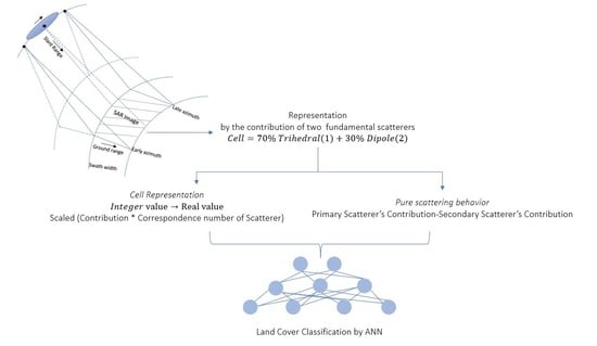
Applying the proposed classification scheme, the Double Scatterer Model is firstly applied to the processed data. Each PolSAR cell/pixel is now presented by a weighted composition of two fundamental scattering mechanisms, in a form analogous to the following:
Each fundamental scattering mechanism can be assigned to an integer number from 1 to 5, as it is shown in
Table 2.
The second and the third stages involve the key innovation points of our research that lie in the assignment of specific intervals of real numbers to each scattering mechanism, thus determining the purity of scattering behavior to each cell.
Fundamental scatterers are now represented by their identical continuous values rather than by a unique integer number, as is shown in
Table 3. This is accomplished by focusing on the contribution of the dominant scattering mechanism in each cell. Specifically, based on the fact that the contribution rate of the primary scatterer is always greater than 0.5, we can assume that each cell is represented by a number resulting from the formula below:
Applying the above to each scattering mechanism located in an interval of continuous values and by performing the appropriate scaling, we can transform these intervals so that each elementary scattering mechanism will be identified in a unique continuous range without overlaps between the intervals.
A much more detailed representation of PolSAR data has now been achieved.
Subsequently, in order to utilize the informational content of the secondary scattering mechanism, the difference between the weights/contribution rates of the primary and secondary scatterers has been calculated for each cell. In this sense, the pure scattering behavior is determined.
According to the above, each cell/pixel corresponds to 2 values, a real number from the interval that determines the fundamental scatterer and a value that represents the purity of the scattering behavior. These features, extracted based on the Double Scatterer Model, will be used in the classification procedure.
The last stage of our process is the classification procedure performed by an ANN. In order to exploit the spatial associations, a pixel window is used to calculate the mean values and the standard deviations of the 2 features in local neighborhoods. Notably, in each land cover a pixel sliding window determines the mean value and the standard deviation of 49 values that correspond to the fundamental scatterer intervals (34) and 49 values that represent the feature of purity (35). In total, 4 features for each neighborhood of pixels/cells will be used in the classifier.
The neural network designed for this research is a fully interconnected linkage of three layers. The input layer is composed of 4 neurons since we use 4 features. Using the
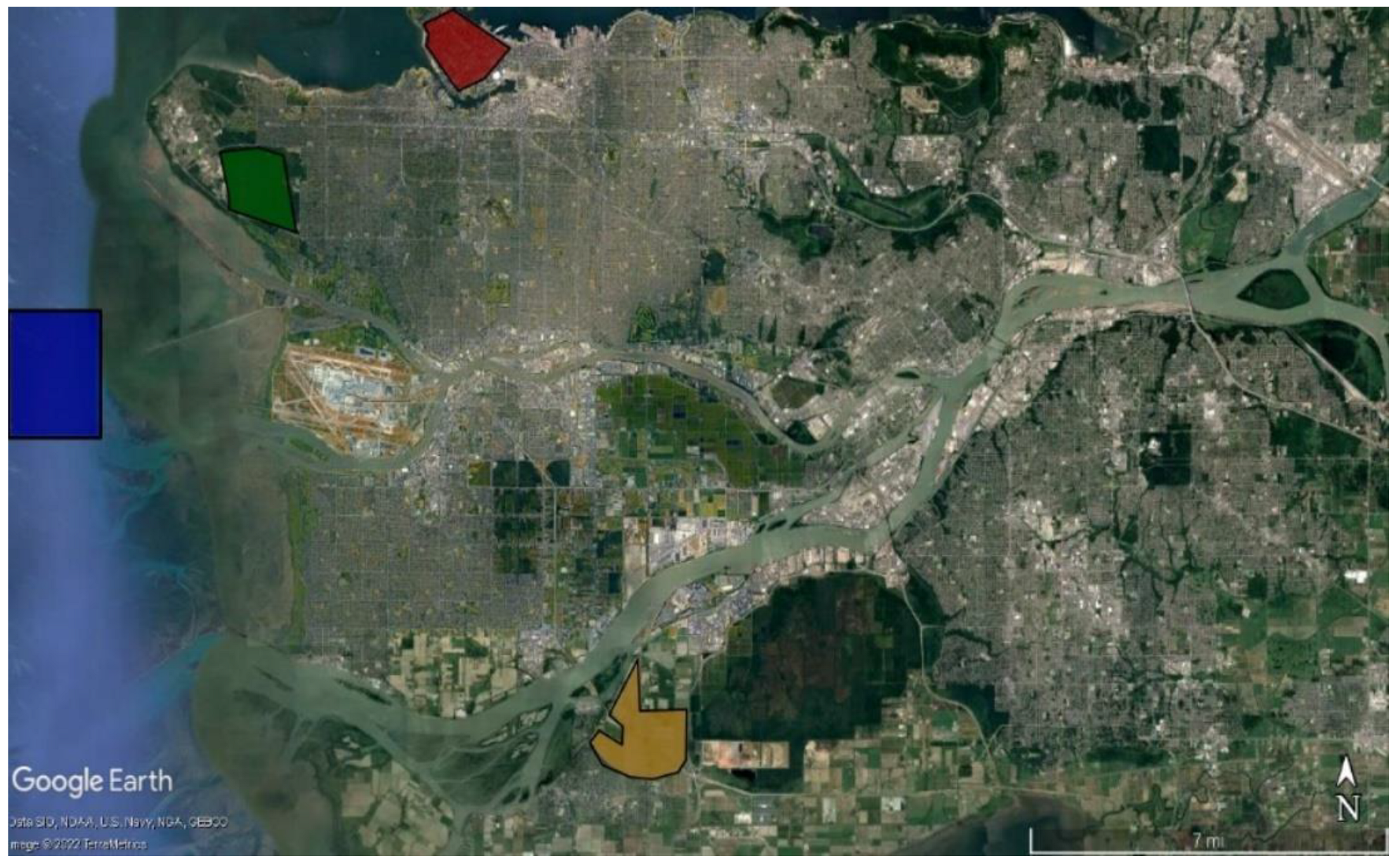
window, the network is able to assimilate data of spatially adjacent pixels, a fact that significantly affects the accuracy of our task since it is utilizing the local neighborhood information of each cell/pixel. The visual classification of imagery by a human involves the use of both spectral and spatial associations, a combination which we attempt to exploit in this study. A single layer including 3 neurons is termed the hidden layer. The selection of both the number of hidden layers and the number of neurons was based on tests on the specific task and on our goal to construct a simple network with the fewest possible parameters. By increasing the number of either neurons or of hidden layers, the model’s complexity increased as well as the computational time of the process, without leading to better results. The output layer is composed of 4 neurons representing the target classes of land covers (sea, urban/built up, dense vegetation, agriculture/pasture) that were to be produced by the network. Every neuron within one layer is fully interconnected with the neurons in the adjacent layers. These interconnections, known as synapses, as mentioned in the previous section, are determined by the activation function, which in our task is the sigmoid function:
The fact that the sigmoid function is monotonic, continuous and differentiable everywhere, coupled with the property that its derivative can be expressed in terms of itself, makes it easy to derive the update equations for learning the weights in a neural network when using the backpropagation algorithm, as in the network we developed. Typically, the backpropagation algorithm uses a gradient-based algorithm to learn the weights of a neural network. In our case, we chose the “adam” optimizer, and a thorough description of this optimization method can be found in the research published by Diederik P. Kingma and Jimmy Lei Ba [
30]. In the designed MLP network, epoch training is used as it is more efficient and stable than pixel-by-pixel training [
31]. One epoch is when an entire dataset is passed forward and backward through the neural network only once. Since one epoch is too big to feed to the computer at once, we divide it into several smaller batches. Batch size is the last hyperparameter determined in the proposed ANN, it corresponds to the total number of training samples that will be passed through the network at one time. In this study, the number of epochs was chosen to be 10.000, which is large enough to gain sufficient knowledge of class membership from the training dataset, but not too large to make the training data overtrained, while the batch size is 128 and causes the model to generalize well on the data. To evaluate the performance of our model on the available dataset, k-fold cross-validation was implemented. The selected data depicted in colors in
Figure 2 are split into K folds with a ratio of 70/30 train/test set, respectively, and are used to evaluate the model’s ability when given new data. K refers to the number of groups the data sample is split into. In our study, the k-value is 5, so we can call this a 5-fold cross-validation.
7. Experimental Results
The results of the proposed classification scheme exceeded our expectations. The process of training and presenting results with the specific parameters mentioned in
Section 6 takes only 11 min. In particular, the average accuracy of the 5-fold cross-validation, using the
pixel window, is estimated to be
. A more in-depth analysis of the results is depicted in the confusion matrix below, in
Figure 7. In order to present the confusion matrix, a random train/test split was used with the ratio of 70/30 for each land cover.
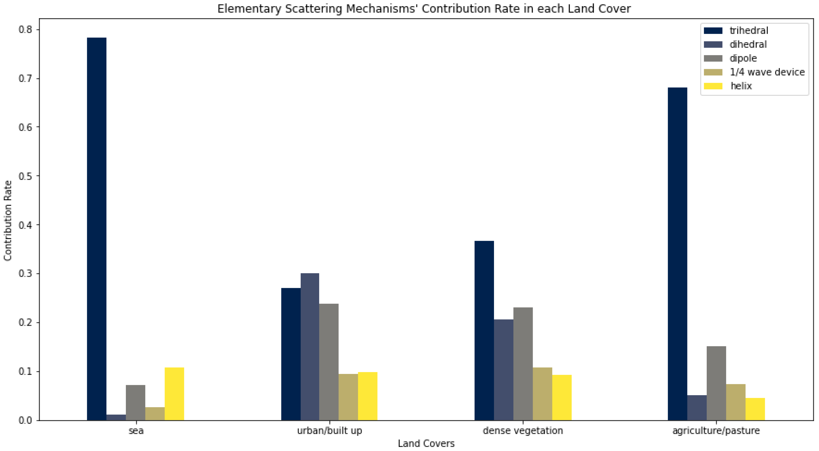
The accuracy rates are very high. The only class that presents lower classification accuracy is the agriculture/pasture land cover. The latter was confused with the sea land cover. It is worth noting that this has been already observed in [
18] and can be explained. In particular, the scattering behavior of agriculture areas and sea land cover is similar, since both cases are flat surfaces. Moreover, the explanation can be supported by
Figure 8, in which the dominance of the trihedral scatterer is clear. The significant difference is the higher rates of the contribution of the trihedral scattering mechanism in sea land cover compared to agriculture/pasture areas, which leads to an accurate discrimination. In
Table 4, the results from recent and well-established land cover classification procedures are reported so that a brief comparison with the present technique can be made for better evaluation.
It can be stated that the overall accuracies (OAs) are very high, but the accuracy per class gives the greatest detail that characterizes each classifier. The proposed classification scheme accomplished an OA of 0.9287 with high rates in each land cover class as well, with the least possible complexity.


