Article

Single or Combine? Tourism Demand Volatility Forecasting with Exponential Weighting and Smooth Transition Combining Methods

1
School of Business and Economics, University Putra Malaysia, Serdang 43400, Malaysia
2
Laboratory of Computational Statistics and Operations Research, Institute for Mathematical Research, University Putra Malaysia, Serdang 43400, Malaysia
3
Faculty of Business, Economics and Accounting, HELP University, Kuala Lumpur 50490, Malaysia
*
Authors to whom correspondence should be addressed.
Computation 2022, 10(8), 137; https://doi.org/10.3390/computation10080137
Submission received: 24 May 2022 / Revised: 20 July 2022 / Accepted: 22 July 2022 / Published: 9 August 2022

Abstract

:
Tourism forecasting has garnered considerable interest. However, integrating tourism forecasting with volatility is significantly less typical. This study investigates the performance of both the single models and their combinations for forecasting the volatility of tourism demand. The seasonal autoregressive integrated moving average (SARIMA) model is used to construct the mean equation, and three single models, namely the generalized autoregressive conditional heteroscedasticity (GARCH) family models, the error-trend-seasonal exponential smoothing (ETS-ES) model, and the innovative smooth transition exponential smoothing (STES) model, are employed to estimate the volatility of monthly tourist arrivals into Malaysia. This study also assesses the accuracy of forecasts using simple average (SA), minimum variance (MV), and novel smooth transition (ST). STES performs the best of the single models for forecasting the out-of-sample of tourism demand volatility, followed closely by ETS-ES. In contrast, the ST combining method surpasses SA and MV. Interestingly, forecast combining methods do not always outperform the best single model, but they consistently outperform the worst single model. The MCS and DM tests confirm the aforementioned findings. This article merits consideration for future forecasting research on tourism demand volatility.

1. Introduction

Tourism has undergone long-term development and expansion, becoming one of the most globally competitive and dynamic markets [1]. Significantly, the United Nations World Tourism Organization (UNWTO) (2019) in [2] observed a significant reality that international tourism continues to expand with greater diversity than global economies, making the tourism industry a global engine of economic growth and sustainability. Therefore, tourism forecasting has gained traction in recent decades, especially considering the fragile nature of tourism services, such as the imbalanced supply and demand, vacant hotel rooms, and airplane seats that cannot be boarded [3,4,5,6,7]. Thus, the time series of tourist arrivals includes multiple non-stability, non-linearity, and complex patterns that reflect the nature of volatility or variation in tourist arrivals [8].
The concept of volatility originated in finance due to the observation that high market returns tend to be followed by large returns, whereas low market returns also appear to be followed by small returns [9]. Tourism forecasting is related to tourism volatility to forecast the tendency of tourism variation. It is defined as the influence of shocks that occur in periods of very high and low activity. These shifts are commonly associated with what is known as “news shocks” [4], such as unpredictable financial recession [10], seasonality changes [11,12], natural catastrophes [13], terrorist attacks [14], and other effects. Utilizing and constructing effective methods for tourism demand volatility forecasting becomes a matter of urgent consideration for the entire tourism industry [15,16].
The desire to reduce risk and ambiguity is the driving force behind the demand for more accurate tourism forecasting [17,18]. Therefore, it is critical to create tourism forecasting models with high accuracy and reliability. Abundant data processing systems have emerged to facilitate the development of a wide range of new approaches to tourism forecasting. The novel methods include time series models, econometric models, artificial intelligence, judgmental forecasting, and combined or hybrid models [19]. Researchers are inclined to use generalized autoregressive conditional heteroscedasticity (GARCH) models to simulate stylized facts when discussing volatility forecasting. Since GARCH models can recreate stylized phenomena, such as volatility clustering, they are widely used to analyze time series data pertaining to financial markets and have achieved satisfactory results [20]. Meanwhile, the autoregressive integrated moving average (ARIMA) model and its offshoots have aroused great interest recently, primarily because of their excellent adaptability and convenience in representing a diverse range of time series. The other reason is that the ARIMA model is built using the Box–Jenkins method, which has high effectiveness in establishing models [21]. An extension model known as SARIMA eliminates non-stationarity in the series through seasonal differencing of the proper order. The SARIMA model is developed for time series data showing seasonal variations. It has been validated that the SARIMA model can fit to the time series data well. Therefore, (S)ARIMA and GARCH approaches are extensively applied to modeling and forecasting. Academics have also focused on several traditional statistical approaches, such as the exponential smoothing (ETS-ES), which has been demonstrated superior to several complicated algorithms [22]. The ETS-ES technique overcomes the shortcomings of conventional ES models. Specifically, ETS-ES predictions are simply weighted averages of past observations. Higher weights indicate more recent observations, and total weights drop exponentially with time. In this study, the smooth transition exponential smoothing (STES) method was employed for forecasting tourism demand volatility for the first time. The STES method allows the change of the smoothing parameter, which is basically a logistic function of a variable specified by the user [23,24,25,26].
It makes sense to use numerous forecast combining methods, providing a new orientation for tourism forecasting research that incorporates the forecasts associated with the single models [27], given that forecast combining is a method that developed by a set of single models lying on a weighting distribution [28]. Another viewpoint is that combining gives the potential for a diversified portfolio of different forecasts [29]. According to empirical research, forecast combining is an effective method for improving the accuracy of tourism forecasting [27,30,31]. In addition to the above-mentioned models, tourist forecasting studies have also investigated simple combination, variance-covariance, and discounted mean square forecast error (MSFE) [32,33,34,35]; weighted combination [9,36,37,38,39,40]; ARIMA-back propagation neural network (ARIMA-BPNN), Naïve-support vector regression (Naïve-SVR), ES-SVR, and ARIMA-SVR methods [41]. Based on the findings of empirical research, to improve the forecasting accuracy of the model, it is necessary to use effective approaches to breakdown the original information and mix linear and nonlinear models throughout the hybridization process. In fact, linear models, such as ARIMA and GARCH, are more capable of forecasting linear and smooth trends [20]. Therefore, GARCH and ES specifications were added to the SARIMA model, and SARIMA-GARCH and SARIMA-ES models were thereby constructed for forecasts of the tourism demand volatility in this paper. Moreover, smooth transition (ST), a new combined approach, was introduced in this research. By modeling the combining weight as a logistic function of one or more transition variables, the ST method enabled the combination to adapt over time to the relative supremacy of various methods [42].
There is a growing body of literature on forecast combining, but it is surprising that research on volatility forecast combining in the tourism section is significantly less developed. The purpose of this study is to close the aforementioned gap by determining if forecast combining methods may improve the tourism demand volatility forecasting accuracy in a practical setting pertaining to the primary source markets of Malaysia’s inbound tourism. Furthermore, this study offers a reliable and realistic volatility forecasting for policy agencies, policymaking, and academic literature. The fact that volatility patterns have a major impact on the forecasting accuracy is a crucial explanation. Forecast limitations (upper and lower bounds) are required to evaluate the impact of extreme shocks and hazards on international tourism demand [43].
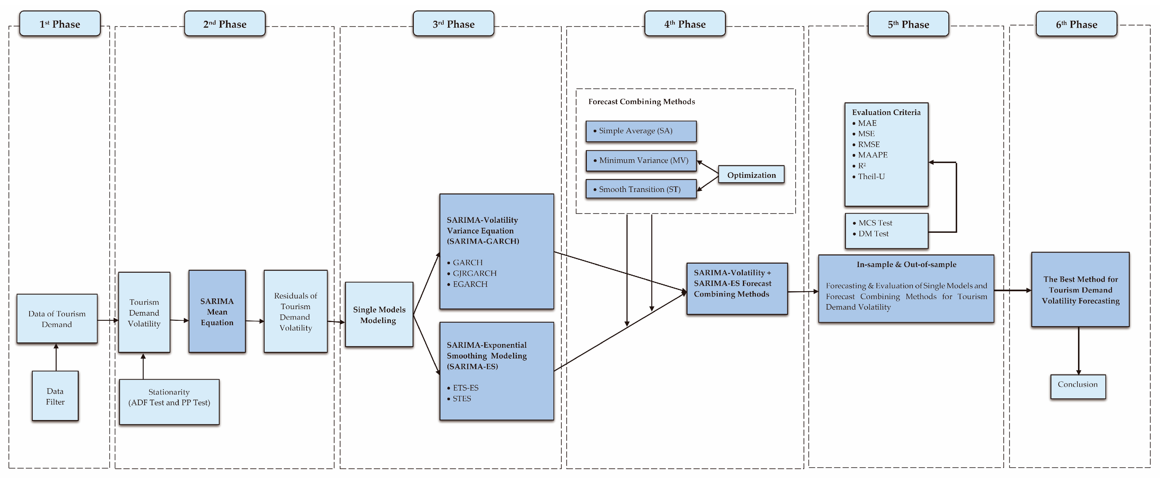
Thus, this research also incorporates innovative methods for combining volatility forecasts. Among them, four modeling methods, namely seasonal autoregressive integrated moving average (SARIMA), generalized autoregressive conditional heteroskedasticity (GARCH), error-trend-seasonal exponential smoothing (ETS-ES), and smooth transition exponential smoothing (STES), are utilized to construct models that forecast tourist arrivals into Malaysia. The prime focus is on the three forecast combining methods, including simple average (SA), minimum variance (MV), and an innovative proposed smooth transition (ST), which has never been considered before in forecasting tourism demand volatility. They are utilized to examine how effective forecast combining is at forecasting the tourism demand volatility. This study analyzes the performance of the GARCH and ES family methods, and their combinations, primarily with respect to three forecast combining methods. The most important contribution of this work is deciphering the forecasting accuracy of forecast combining and single forecasts in tourism demand volatility and discovering the optimal method for forecasting tourism demand volatility in Malaysia.
The remaining sections of this study are organized as follows. Section 2 discusses current research in tourism forecasting and modeling, and the yield of forecast combining methods. Three forecast combining methods, four volatility models, two exponential smoothing methods, and evaluation measures of forecasting accuracy are introduced in Section 3. In Section 4, the data sources and research methodology are explained. Section 5 and Section 6 examine, respectively, the in-sample outcomes associated with the methods and the out-of-sample outcomes. Section 7 summarizes this study.

2. Literature Review

2.1. Tourism Forecasting Methods

Diverse methods have been utilized to forecast tourism demand, with the majority of these studies employing time series models, econometric models, artificial intelligence models, judgmental forecasting, and combining methods [7,44]. Before the 1990s, tourism forecasting was conducted using conventional regression methods [27]. Since the mid-1990s, numerous methods for enhancing the accuracy of tourism forecasting have been described [4]. The application of time series and econometric models is widespread [45,46,47,48]. Several tourism research have incorporated financial literature’s volatility models to forecast tourist data [27,43,49,50,51,52,53,54,55,56,57,58].
The ARIMA model, which is generally adapted to more prolonged journey movement, is at the core of this category of methods [9]. The implementation of seasonal ARIMA models has grown in recent years. Indeed, Kim and Moosa (2005) in [59], Kulendran and Wong (2005) in [57], Papatheodorou and Song (2005) in [60], Song and Li (2008) in [61], Wu et al. (2021) in [62], and Zhang et al. (2022) in [63] all used it to analyze the importance of seasonal fluctuations to tourism streams. All three ARIMA with exogenous variable (ARMAX) models greatly outperformed their ARMA counterparts in Google search data hotel room demand forecasts, according to Pan et al. (2012) in [64]. Tsui et al. (2014) in [65] utilized the SARIMA model and the ARIMAX model to forecast Hong Kong (China) airport passenger traffic. SARIMA, artificial intelligence (AI) model selection and other methods were employed by Akın (2015) in [66] to forecast monthly tourist arrivals to Turkey from various countries. SARIMA was used to identify Andalusian oleotourism solutions that match the criteria of the target market and deliver an environmentally beneficial and economically viable product, according to Millán et al. (2018) in [67]. Msofe and Mbago (2019) in [68] discovered that the SARIMA model was the best fit for foreign tourist arrivals in Zanzibar. Abu et al. (2021) in [69] employed SARIMA and ES to forecast the demand for ecotourism. The results suggest that the SARIMA model outperforms the exponential smoothing.
Since the early 1990s, volatility models have been actively utilized in finance and econometrics research. Engle (1982) in [70] and Bollerslev (1986) in [71] were key publications on which the models were built. Note that the generalized autoregressive conditional heteroskedasticity (GARCH) family models were also developed to investigate and model time-varying volatility forecasting in financial time series [71,72,73,74,75,76]. However, according to Chang et al. (2009) in [77], tourism demand volatility analysis still is a noticeably newer method in tourism research. The studies (Balli and Tsui (2016) in [78]; Balli et al. (2019) in [43]; Coshall (2009) in [9]; Coshall and Charlesworth (2011) in [37]; Divino and McAleer (2010) in [55]; Kim and Wong (2006) in [4]; Song and Li (2008) in [61]) show that tourism demand volatility modeling and forecasting have been carried out, especially adopting the GARCH family models. For instance, Chan et al. (2005) in [49] utilized ARMA-GARCH for static or constant conditional correlation volatility models. Chang et al. (2011) in [52] used multivariate conditional volatility models to examine the association between international tourism demand as defined by tourist arrivals and their related volatility in the four most significant Association of Southeast Asian Nations (ASEAN) locations. ARIMA, GARCH, and an ARIMA-GARCH hybrid were all employed by Chhorn and Chaiboonsri (2017) in [79] to forecast tourist arrivals. Using a GARCH model, Hwang et al. (2018) in [80] assessed the link between the climate volatility index (CVI) and Japanese tourist arrivals in Korea. Using SARIMA with exogenous variables (SARIMAX) and GARCH volatility models, a study estimated air tourist arrivals from New Zealand’s eight most important source markets [43]. Santamaria and Filis (2019) in [81] used a dynamic conditional correlation-GARCH (DCC-GARCH) model to assess the relationship between tourism growth and destination macroeconomic conditions. The ARMA-GARCH model was utilized by Makoni and Chikobvu (2021) in [82] to improve forecasting capacity and can capture and quantify volatility. Ampountolas (2021) in [83] assessed typical time series forecasting models for daily demand at many horizons utilizing Holt–Winters (HW) triple exponential smoothing, SARIMAX, GARCH, and GJRGARCH. GARCH and GJRGARCH provide more accurate predictions over horizons.
Furthermore, exponential smoothing (ES) models are less commonly cited in the research on tourism demand volatility, notwithstanding the overwhelming evidence that ES frequently produce reasonable forecasting of orientation and trend shifts in tourism demand [3,14,54,84,85]. Just like Cho (2003) in [54], Coshall (2009) in [9], Coshall and Charlesworth (2011) in [37], and Lim and McAleer (2001) in [86] analyzed the performance of the ES method in forecasting tourist arrivals. Especially, Hassani et al. (2015) in [84] contrasted singular spectrum analysis with ARIMA, exponential smoothing (ETS), and neural networks (NN) for tourism demand forecasting. Xu et al. (2016) in [87] employed Naïve 1, simple exponential smoothing (SES), double exponential smoothing (DES), ARIMA, and other approaches to estimate tourist arrivals in Hong Kong (China). Annual international tourist arrivals in Zambia were examined by Jere et al. (2019) in [88] using ARIMA and Holt–Winters exponential smoothing (HWES). According to the results, HWES is a suitable forecasting model with a decent degree of forecasting accuracy. For the fluctuating number of international tourists visiting North Sumatra, Febrian et al. (2019) in [89] compared double moving average (DMA) and double exponential smoothing (DES).
However, the previous ES models appeared to generate volatile forecasts and performed inadequately in empirical research. Thus, Taylor (2004) in [23,24] mentioned smooth transition exponential smoothing (STES), a novel method towards forecasting volatility, which allows for the construction of a smoothing parameter using a logistic function within a user-defined variable. It is a simple method for volatility forecasting to evaluate the variance being a simple moving average among the squared shocks in the past. Both the size that takes the absolute or squared value of raw data and the sign that is the raw data itself are permitted. Despite this, the news impact curve of STES exhibits complicated asymmetries when both the magnitude and sign of past errors are used as transition variables. By conducting volatility forecasting in the worldwide eight major stock markets, Taylor (2004) in [23,24] concluded that STES with time-varying parameter outperforms most of the GARCH-type models. Moreover, simulation and empirical investigations demonstrate that STES outperforms other switch transition GARCH models, such as logistic smooth transition-GARCH (LSTGARCH) and exponential smooth transition-GARCH (ESTGARCH) [25]. Despite the existing research on the application of STES, to the best of our knowledge, no study examining the performance of STES has been published in the literature on tourism forecasting.

2.2. Tourism Forecast Combining

Using the Web of Science search engine, we discovered just 29 papers on the topic of forecast combining methods for tourism forecasting from January 1980 to January 2022. It is evident that this research subject requires further investigation, particularly in terms of combining tourism demand volatility forecasting. Among them, a few other types of research hire forecast combining methods throughout the tourism field. In tourism forecasting, empirical results indicate that neither single model can produce the most accurate forecasting of widespread occurrences [49,61]. Comparatively, the accuracy of forecast combining is significantly greater than the accuracy of the worst unified forecasts model or the average accuracy of single forecasts, like the ARIMA model, vector autoregression (VAR), error correction model (ECM), and autoregressive distributed lag model (ARDL) by Wong et al. (2007) in [27]. Adopting the SARIMA, ARDL, ECM, VAR, combining method (simple average), and discounted mean square forecast error (Discounted-MSFE), Song et al. (2009) in [31] analyzed the ten main tourist arrivals to Hong Kong (China). The case study of Shen et al. (2008) in [17] produced single models (seasonal Naïve, SARIMA, etc.) and forecast combining methods (e.g., simple average, variance-covariance, and time-varying-parameter combining methods) for forecasting tourism demand from the UK to seven main destinations. In another example, to forecast monthly Vienna tourist arrivals, Önder and Gunter (2016) in [90] employed MA, ETS, Naïve, and combining methods (forecast encompassing uniform and Bates–Granger weights). Years later, Li et al. (2019) in [28] used single models, such as Naïve, ES, SARIMA, and interval combining methods, to investigate Hong Kong (China) tourism demand. Hu and Song (2020) in [91] applied an artificial neural network (ANN) model to incorporate causative factors, search engine data, and historical tourism demand. This aims to see if integrating causative factors with search engine data might enhance forecasting. Single and combining methods for projecting EU tourism demand were examined by Gunter et al. (2020) in [35], using ARIMA, RE-GARIMA, ETS-ES, and forecast combining (Bates–Granger weights and uniform weights). Ma (2021) in [39] employed the Grey prediction model, BP neural network, and weighted combination (parallel combination model and series combination model) to explore whether combined forecasts outperform single forecasts for the development law of China’s domestic tourism. Wu et al. (2021) in [62] found the SARIMA + LSTM forecast method outperforms other methods. He et al. (2021) in [92] SARIMA-convolutional neural network-long short-term memory network (SARIMA–CNN–LSTM) model to forecast tourism demand data at daily frequency. The results confirmed that the new model yields greater forecast accuracy than the single models.
Combining methods have been implemented in tourism forecasting, according to the above analysis, but their applications are limited to forecasting tourism demand. Thus, there has been far less research on the application of tourism demand volatility forecasting. Specifically, just regarding the tourism forecasting case of Coshall (2009) in [9], using Naïve 2, ES, ARIMA-GARCH, and combining methods (ARIMA-GARCH, ES) to forecast the UK tourism demand to overseas destinations, represents a unique demonstration of volatility forecast combining with the ES model such that neither of the single models is more precise than the combining methods. Meanwhile, Coshall and Charlesworth (2011) in [37] further employed almost the same methods for the goal programming approach to forecast combining. This study intends to address the knowledge gap in the field of tourism demand volatility by employing innovative single and combining methods to increase the accuracy of forecast combining.

2.3. Volatility Forecast Combining

In out-of-sample evaluations, no other method consistently surpassed the simple average (SA) forecast combining method. In addition to using expert estimates, SA is competitive when employing model-based forecasting [93]. Bates and Granger (1969) in [94] were the pioneers to mention using minimum variance (MV) forecast combining as a means of increasing precision. This method is also termed optimal weights (OW). The weights are determined using a method of estimation known as least squares and any available historical data on forecasting error. Due to its design to limit in-sample error variance, OW is superior to all other linear weighting methods when applied in-sample. Because estimated weights are highly fitted to training data and susceptible to sampling-based volatility, out-of-sample performance is not necessarily superior. Due to structural changes in time series, the performance of MV and SA varies over time. In terms of forecast combining, the SA method is the simplest since, unlike more complex models such as MV, no parameters are ever specified while utilizing the SA method. Notably, after that, Becker and Clements (2008) in [95], Degiannakis (2018) in [96], Doidge and Wei (1998) in [97], Dunis and Huang (2002) in [98], Granger and Ramanathan (1984) in [99], Kroner et al. (1995) in [100], Pesaran and Timmermann (2007) in [101], Yang et al. (2015) in [102], and Yang et al. (2017) in [103] suggested that combining has a great deal of opportunity for improvement in terms of reducing the variation that results from selecting a unified model. Consequently, most published studies pointed to the efficacy of combining methods in volatility forecasting. Yet, the aforementioned two methods have been employed less frequently in the field of tourism forecasting.
However, almost all volatility forecast combining methods involve fixed combining weights, the one exception being the study by Preminger et al. (2006) in [104]. Deutsch et al. (1994) in [105] introduced a novel method for adding time-varying combining weights into the intuitive and simple least-squares regression framework. Their method of combining is a smooth transition (ST) regression model. In smooth transition investigations, nonlinearity in the mean equation is far more pronounced [106]. Significantly, the statistics define the timing of the change in volatility without the researcher’s intervention. By parameterizing the transition function, it is possible to compute the timing of the transition to a new state. This function is used to evaluate time-varying coefficients in research on smooth transition [107]. Meanwhile, the model is highly adaptable based on transition variables because the models grab unconditional and conditional heteroskedasticity [42]. The change in regimes of volatility can be endogenized or correlated with significant economic indicators. They could be formidable competitors to exogenously driven heteroskedasticity restrictions given their advantages [108]. Therefore, we utilized this concept to account for the heteroskedasticity of the data in the tourism sector. Notably, the ST combining method establishes the combining weight as the logistic function of a transition variable. This method permits the combination to adjust over time to the relative superiority of the different methods by modeling the combining weight as a logistic function of one or more transition factors. In this manner, the method permits the combining weight to progressively vary based on a given condition. A highly developed statistical analysis of the smooth transition combining method is accessible for further work. However, to our knowledge, the only study that has considered this form of combining is that of Taylor and Majithia (2000) in [109], not in the tourism area.

3. Methods Description

3.1. Individual Volatility Forecasting Methods

The generalized autoregressive conditional heteroscedasticity (GARCH) modeling procedure typically consists of a mean equation and a volatility equation, both of which can be estimated simultaneously using the maximum likelihood method. This method stresses the regularity of conditional variance because short-term volatility forecasting based on existing information is frequently timelier and more accurate. Moreover, the volatility equation in the GARCH model has autoregressive and moving average structures, allowing it to forecast the conditional variance. All volatility models begin with a “mean equation”, which, depending on the situation, is typically a normal ARIMA (as in this case) or regression model. This study employs the SARIMA mean equation and the GARCH family variance models for the single and forecast combining modeling.

3.1.1. Seasonal ARIMA (SARIMA)

The seasonal autoregressive integrated moving average (SARIMA) is a derivative of Box–Jenkins method (1976) in [110], in which the seasonality of series is supported through seasonal difference. The full formulation of a multiplicative seasonal ARIMA model as the general form SARIMA (p, d, q) (P, D, Q)S: the nonseasonal and seasonal factor parameters are enclosed in parentheses, respectively. SARIMA was enhanced in this study via integrating the notion of volatility [5], which was termed as “SARIMA-volatility” models throughout the whole research.
  ϕ p B Φ P B s 1 B d 1 B s D Y t = Θ 0 + θ q B Θ Q B s ε t  
where each terminology in turn explicitly stipulates B is the backshift operator; Θ 0 is a constant and ε t is the white noise. ϕ p B is the nonseasonal AR operator; θ q B is the nonseasonal MA operator; Φ P B s is the seasonal AR operator and Θ Q B s is the seasonal MA operator. 1 B d is the nonseasonal differencing of order d and 1 B s D   is the seasonal differencing of order D. Y t is the forecasting value for the period t and s equivalents 12 months. Seasonal changes are vital to the stability of any series. Trend stationarity is an additional factor to consider while applying SARIMA. Thus, this model may be used to get the optimal mean equation for each of the 17 tourist arrivals.

3.1.2. SARIMA-GARCH Family Models

By far one of the most influential models for volatility conditional variance modeling and forecasting is generalized autoregressive conditional heteroscedasticity (GARCH) [71], which is generally recommended for a significantly more flexible lag structure. The conditional mean equation and variance equation are jointly estimated in GARCH family models for forecasting the monthly returns of tourism demand volatility in Malaysia. In the GARCH family of models, order = 1 has shown that a short lag is sufficient to construct variance models over a rather lengthy sampling period [111,112,113]. Consequently, GARCH (1,1), EGARCH (1,1), and GJRGARCH (1,1) are applied in this study by analyzing the logarithmic regression in-sample data set of each tourism demand volatility series. The conditional variance GARCH (1,1) model is described as follows:
  σ t 2 = ω + α 1 ε t 1 2 + β 1 σ t 1 2    
where ω denotes constant parameters; α 1 and β 1 are the coefficients; ε t 1 2 is the ARCH term, which means volatility news from the previous period; σ t 1 2 is the GARCH term, which is the forecasting variance from the previous period. Especially, σ t 2 is the one-period-ahead forecast variance based on past information and is called the conditional variance. Where ω > 0, α 1 ≥ 0 and β 1 ≥ 0 for the positive variance. 0 ≦ α 1 + β 1 < 1 for the stationarity of variances.
Despite its success, GARCH fails to capture asymmetric volatility in tourism forecasting. In the formula, the conditional variance is typically determined by the amplitude of the lagged residuals rather than their sign. However, this limitation has been removed by introducing more adaptive volatility treatments that account for the asymmetric volatility resulting from positive and negative shocks [112,113,114,115]. Two simple categories of models that capture the asymmetric behavior of returns are the exponential GARCH (EGARCH) model [116] and GJRGARCH [117]. Thus, it is worthwhile to analyze if a negative shock to the tourism sector causes fluctuations to rise more dramatically than a corresponding positive shock of the same magnitude.
The EGARCH model can capture news shocks effects that the GARCH model is unable to do so, that is, the negative shock at t − 1 has a stronger effect on the variance at time t than the positive shock. EGARCH does not enforce any constraints into the parameters to maintain steadiness only inside the conditional variance rationale [116]. The specification for the conditional variance EGARCH (1,1) model is:
  ln σ t 2 = ω + α 1 ε t 1 σ t 1 + ϕ 1 ε t 1 σ t 1 + β 1 ln σ t 1 2  
where ω denotes constant parameters; α 1 , β 1 , and ϕ 1 are the coefficients; the log of the conditional variance is denoted by ln σ t 2 . One element that may have helped to the broad adoption of EGARCH is the conditional variance. It is no longer necessary to impose constraints on the parameters in order to guarantee a positive conditional variance because the function is exponential. Additionally, the model allows for asymmetries via the ϕ 1 term in Equation (3). If ϕ 1 = 0, the model is symmetric; if ϕ 1 < 0, volatility increases because of the negative shocks; and if ϕ 1 > 0, this indicates the absence of a leverage effect but implies that a positive shock affects volatility more than negative shocks. In addition, the leverage impact is exponential rather than quaternion, thus conditional variance forecasts will always be positive [9]. This indicates that the leverage effect is exponential rather than quadratic, ensuring that forecasts of conditional variance are positive. This is one of the factors that led to EGARCH’s selection for this inquiry.
A widespread simple asymmetric GJRGARCH from Glosten et al. (1993) in [117] makes it possible for the conditional variance to react distinctly towards the negative and positive advancements or news when the leverage effect is assessed. The conditional variance GJRGARCH (1,1) model is given by:
  σ t 2 = ω + α 1 ε t 1 2 + γ 1 ε t 1 2 d t 1 + β 1 σ t 1   2  
where ω denotes constant parameters; α 1 , β 1 , and γ 1 are the coefficients;   d t 1   is dummy variable. d t 1 = 1 if a negative shock exists, represented by ε t 1 < 0; and d t 1 = 0 if a positive shock exists, represented by ε t 1 > 0. Good news and bad news have different effects on the conditional variance, which is measured by the coefficient γ. In most cases,   γ 1 > 0 is observed, pointing out the existence of the leverage effect (a negative shock increases tourism demand volatility). Thus, in addition to using these three volatility models for the fluctuation of inbound tourists to Malaysia modeling, we also use them to analyze whether some news shocks have a symmetric and asymmetric impact on inbound tourists. This is to help Malaysian tourism-related developers make corresponding travel plans and strategies, based on the forecasting results.

3.1.3. SARIMA-Exponential Smoothing (ES) Family Methods

Error-Trend-Seasonal Exponential Smoothing (ETS-ES)

Squared residuals from the SARIMA model were extracted by exponential smoothing (ES) via integrating the notion of volatility, termed as “SARIMA-ES” models throughout the entire research. Among them, ETS-ES is defined by Hyndman et al. (2002) in [118] as an expanded class of exponential smoothing (ES) methods (e.g., Holt–Winters’ additive, multiplicative and damped methods shown in Table 1). Model selection and forecasting standard error can be calculated theoretically, allowing state-space likelihood estimates to be used to examine these models by Hyndman and Khandakar (2008) in [119]. This ETS-ES algorithm overcomes limitations from the previous models of exponential smoothing. In a nutshell, ETS-ES forecasts are weighted averages of previous observations, with the higher weight being assigned to the more recent record and overall weights decaying exponentially. In other words, these weights are exponentially decreasing. The whole family of ETS-ES models can be distinguished by the three major parameters: the error, trend, and seasonal components, each of which can be either additive (A), multiplicative (M), or none (N), with a total of 30 models for the various possible combinations of error, trend, and seasonality in Table 2 [120]. Meanwhile, Athanasopoulos et al. (2011) in [44] found that the ETS-ES performed particularly well for monthly data in their tourism forecasting competition. Thus, we employed the “EViews 11-automatic selection” of the ETS-ES models to fit exponential smoothing models and evaluated possible alterative models prior to selecting the best-performing model to simulate the data for Malaysian tourism demand volatility modeling.

Smooth Transition Exponential Smoothing (STES)

Exponential smoothing is a common and practical method for volatility forecasting. Several additional authors have stated that a time-varying smoothing value could potentially capture the time series’ most significant present changing characteristics. Taylor (2004) in [23,24] proposed smooth transition exponential smoothing (STES), which is the subject of this investigation, here borrowing it for the first time to conduct model combining testing to determine whether it outperforms other models with regards to Malaysia’s tourism demand volatility. The method was formulated as:
  σ ^ t 2 = α t 1 ε t 1 2 + 1 α t 1 σ ^ t 1 2
where
α t 1 = 1 1 + exp β + γ V t 1    
α t 1 is the adaptive or smooth transition parameter (modeled as a logistic function), which limits to a range of 0 and 1. The logistic function can adjust itself in accordance with the changes that occur in the transition variable V t 1   . σ ^ t 2 is a function of the calibration of the adaptive smoothing parameter α t 1 , which in turn is dependent on the selection of the transition variable and the optimization (with the help of a solver) of the parameters β and γ (coefficients of the transition variables concerned). We proposed ε t 1 , ε t 1 , ε t 1 2   and their combinations as transition variables for the different STES methods in Table 3. Thus, in contrast to most other current adaptive methods, STES focuses on the process to modulate the adaptive smoothing parameter whilst also estimating β and γ from earlier in this thread affirmation for α t 1 . This method permits the simultaneous capturing of smooth exogenous and endogenous nonlinearity.
The total amount of “squared” in-sample one-step-ahead forecasting error among both actual variance and forecasts has been kept to a minimum for in-sample parameterization forecasts of STES.
M i n t = 1 n   ε t 2   σ ^ t 2 2  
Taylor (2004) in [23,24] discovered that the STES method, when applied jointly with the sign ( ε t 1 ) and size ( ε t 1 or ε t 1 2 ) being transition variables, met or exceeded fixed-parameter exponential smoothing, and that a various assortment of linear and non-linear GARCH family models in out-of-sample volatility forecasting. All these transition variables might have been utilized singly or in combination to generate various STES. The effectiveness of STES is attributed to the evolutionary essence of the time-varying parameter, which contributes to a decrease in the outlier’s prominence by assigning a lower weight primarily to the outlier [23,24,25,26]. For this reason, STES was employed to determine whether forecast combining methods consistently outperform single forecasts.

3.2. Forecast Combining Methods

3.2.1. Simple Average (SA)

There has been considerable literature on the forecast combining since Crane and Crotty (1967) in [121], who proposed the combining of forecasts through regression, and Zarnowitz (1967) in [122], who proposed the simple average (SA) of several forecasts. Researchers tested the forecasting accuracy of other strategies in combining with this to simulate tourism demand volatility. Moreover, when forecast combining given by two or more models, it is vital to determine the weights that will be distributed to each model. The simplest method for combining forecasts is the simple average. In this research, simple average is described as follows:
f t , c = f t , 1 + f t , 2 2
where f t , c is combined forecasts for period t; f t , 1 is the first single forecast for period t; f t , 2 is the second single forecast for period t. In the SA forecast combining method, the weight of the combination is allocated equally among the forecasts. In addition to model-based forecasting, SA forecast combining is competitive. Previous research has demonstrated that this method performs as well or better than more complex forecast combining methods [123]. However, the groundbreaking study by Bates and Granger (1969) in [94] has substantially influenced the development of many interesting combining methods. The studies by Reid (1968) in [124] and Bates and Granger (1969) in [94] generated the impetus for the advancement of theory in forecast combining.

3.2.2. Minimum Variance (MV)

Bates and Granger (1969) in [94] suggested the combining “optimal” method, in which the linear weights are cyphered to lessen the error variance. This method will be to test the “varying weights” method against the “fix weights” method for tourism demand volatility forecasting. The minimum variance (MV) method was formulated as:
f t , c = w t f t , 1 + 1 w t f t , 2
where f t , c is combined forecasts for period t; f t , 1 and f t , 2 are individual forecasts for period t; the weights w t are restricted to be within [0,1], negative weights might well occur in certain instances, given the presence of relationships even amongst the forecast error [124,125]. In this method, the weights have always been quantified using a covariance matrix in which the variances represent the accuracy of individual forecasts, and the covariance reflects their dependence [27]. Consequently, this study will investigate whether the models with varying weights provide the most accurate model for forecasting changes in the number of visitors to Malaysia.

3.2.3. Smooth Transition (ST)

Under the tourism demand volatility forecast combining area, we provided for the first time a new smooth transition, changing weights to combine forecasts of volatility from two distinct methods. This was taken from the smooth transition (ST) forecast combining method [105]. The time-varying combining weight can develop as a logistic function of various transition variable selections. The resulting combining volatility forecasts model is:
f t , c = w t f t , 1 + 1 w t f t , 2
where
w t = 1 1 + exp β + γ V t 1
where f t , c is combined forecasts for period t; f t , 1 and f t , 2 are individual forecasts for period t; β and γ are parameters; V t 1 is the transition variable, which controls the change in the weights. The logistic function enables the value of the time-varying parameter to evolve and adapt according to the changes in the transition variable,   V t 1 . If the coefficients of V t 1 in the exponential expression, β and γ are positive, the logistic function is a monotonically decreasing function of V t 1 . Hence, as V t 1 increases from a large negative value to a large positive value, the impact of the combining forecast,   f t , c , will gradually shifts from the first individual forecast, f t , 1 to the second individual variance forecast, f t , 2 . Put it in another words, the weight on f t , 1 varies from near 1 to near 0, and correspondingly the weight on f t , 2 varies from near 0 to near 1. Thus, we put more weight on f t , 1 rather than f t , 2 . Significantly, there is a variety of candidates for V t 1 . Two obvious suggestions are the sign of past shocks, ε t 1 and the size of past shocks, ε t 1 2 . The sign of past shocks or lagged error term, ε t 1 , was used by Hagerud (1997) in [126] and González-Rivera (1998) in [127], just being a transition variable inside a model of the asymmetry in volatility further identified as its “leverage effect”. The size of the past shocks or the square of the lagged error term, ε t 1 2 , was applied by Hagerud (1997) in [126] as a transition variable to enable an even more adjustable modeling of conditional variance dynamics. Aside from these, ε t 1 was considered as the transition variable in the methods that we referred to as ST1, ST2, and ST3, respectively, for tourism demand volatility forecasting. These combinations of transition variables in smooth transition forecast combining methods, namely ST4, ST5, and ST6, were also introduced in this research. The trade volume, which impacts volatility and predictability, is an additional desirable candidate for the transition variable in the logistic function. This is the first study to use tourism forecasting to investigate whether the ST forecast combining method is superior to other methods.

3.3. Measures of Forecasting Accuracy

Accurate error forecasting and estimation of the future are crucial to the performance of a forecast. While evaluating the quality of the forecasting, no single assessment method can accurately forecast the out-of-sample forecasting error [61]. This is because different forecasting models have varying standards, characteristics, and purposes. Thus, this research will incorporate different measures to improve the forecasting accuracy.

3.3.1. Evaluation Criteria

Notably, if the actual values are less than one, certain evaluation criteria will produce extremely large outliers, and actual values of zero will result in infinite values. In the meantime, the topic of this study is “volatility”, which refers to the fact that the actual changes in tourist arrivals data are close to zero, which can lead to the observation of outliers. Thus, to assess the accuracy of various forecasting methods, we utilized appropriate core evaluation criteria to assess the accuracy of the forecasts: mean absolute error (MAE), mean squared error (MSE), root mean squared error (RMSE), mean arctangent absolute percentage error (MAAPE), R-squared (R2), and Theil-U.
M A E = 1 n t = 1 n y t y ^ t
M S E = 1 n   t = 1 n y t y ^ t 2  
R M S E = 1 n t = 1 n y t y ^ t 2
M A A P E = 1 n   t = 1 n arctan y t y ^ t y t  
  R 2 = t = 1 n y ^ t y ¯ 2 t = 1 n y t y ¯ 2  
  T h e i l U = t = 1 n y ^ t y t 2 t = 1 n ( ( y ^ t ) B M y t ) 2
where n is the total forecasting number of tourists; y t represents the actual number of inbound tourists into Malaysia; y t ^ indicates the forecasting number of inbound tourists into Malaysia;   y ¯ represents the mean of tourist arrivals sample; ( y t ^ ) B M is the benchmark forecasting [76]. MAE is a metric that measures the deviation between forecasting and actual values. MSE is commonly employed as a regression loss function, despite its sensitivity to outliers. RMSE is more sensitive to extreme values than MAE, and it measures the difference between forecasting and actual values. MSE and RMSE give a quadratic loss function and serve as gauges of forecasting uncertainty. In addition, a novel measure of accuracy, mean arctangent absolute percentage error (MAAPE) [128], was introduced for the first time in the tourism forecast combining research domain. MAAPE is independent of scale, intuitive, and simple to compute. Using the arctangent function prevents MAAPE from reaching infinity due to the function’s limited range. MAAPE has the potential to be an incredibly valuable instrument when major errors are caused by inaccurate or erroneous observations. Therefore, it is better suitable for evaluating the performance of volatility forecasting systems in the tourism sector. The coefficient of determination, R2, provides a straightforward method for analysing the accuracy of an estimation or forecasting. It is derived by running a regression between the actual volatility experienced and the forecasting volatility out-of-sample. Additionally, the R2 can be interpreted as a measure of the amount of information contained in the volatility estimator. The model will be more accurate if R2 is closer to unity. Since U-statistic is insensitive to linear transitions and has a standard error of forecasts, it is a good approach to evaluate a forecasting method [12,76,98].

3.3.2. MCS Test

In addition to the summary accuracy metrics, further tests based on several evaluation criteria will be conducted to provide a more precise result. The model confidence set (MCS), addresses the difficulty of selecting the optimal forecasting model from a set of case volatility models. According to Hansen et al. (2003, 2011) in [129,130], the MSC test is a tool for selecting the “best” forecasting model and that of other volatility models for the application of an out-of-sample assessment underneath a loss function. By calculating the MCS for the set of models, the MCS for the set of models that includes the forecast combining as an additional model may be produced and compared to determine whether the combined forecasts outperform the single forecasts. In a large collection of forecasts, there should be just one MCS if the forecast combining exceeds the other forecasts. Thus, unlike other commonly used comparison methods, it is not necessary to define the benchmark model in advance. The MCS test allows users to define their own loss functions based on their research. MCS test has no restrictions on the selection of loss functions. This offers the MCS test substantial versatility.
The MCS test is applied to generate “better” models, which are known as “superior set models” (SSM). Supposing that we originally have a large model set, M 0 , the number of models included in M 0 is x . Thus, we specifically have model m 1 , m 2 ,   m 3 ,…,   m x to be compared and evaluated. The objective of the MCS test is to identify the SSM in which all models have equal predictive ability (EPA). Consequently, the null hypothesis of the MCS test is that all models possess the same forecasting power. The SSM is obtained in accordance with a specific confidence level 1 α . Formally, let M 1 α denote the SSM at the end of evaluation. Assuming that the number of models in the SSM is y , where y x since SSM is obtained through a bootstrap sequentially process of eliminating poorest performed models. After eliminating all poorly performing models, the number of models in SSM is less than or equal to the original model set. According to Bernardi and Catania (2019) in [131], the best-case scenario for SSM is that it consists of a single model or y = 1, as most researchers want to accomplish. Similar as Hansen’s SSM, the MCS data set searches for a model M in which the model i is given preference over other viable alternatives j for a given loss function Li. The null hypothesis has been represented as follows: Ho:   E d ij = 0, where E d ij = L i   L j , for all j in M 0 , j ≠ i , with M 0 the whole models to be evaluated. Even a specific model i would go into the set M when E d ij ≤ 0 for all j in M 0 , j ≠ i   [132].

3.3.3. DM Test

This study utilized the Diebold and Mariano (DM) test [133] to investigate the forecasting accuracy of two competing forecasting models for the Malaysian tourism demand volatility by comparing the root mean squared error and mean absolute error. These tests are shown to be robust to forecast non-normality, bias, and serial correlation, and adaptable to a range of loss structures. Moreover, they are dependent on the variations between loss functions. There is no requirement that a loss function be quadratic or symmetric, and model forecasting errors can be non-Gaussian, non-zero-mean, serially correlated, and contemporaneously correlated [134]. Thus, the Diebold–Mariano (DM) test statistic for comparisons is the simple ratio, and the null hypothesis is that “method 1” and “method 2” have equivalent forecasting accuracy. If the loss differential equals zero, two models have the same forecasting accuracy in this research. The DM test is based on the loss differential:
d 12 t = L e 1 t L e 2 t  
  H 0 : E L e 1 t = E L e 2 t   o r   H 0 : E d 12 t = 0  
d ¯ 12 = 1 T t = 1 T d 12 t
D M = d ¯ 12 σ ^ d ¯ 12 ,   DM ~   N 0 , 1
where e 1 t is the forecast error of method 1; e 2 t is the forecast error of method 2;   d 12 t is the loss differential at time t;   d ¯ 12 is the sample mean of d 12 t ; and σ ^ d ¯ 12 is a consistent estimate of the standard deviation of d ¯ 12 .

4. Data Description and Modeling Derivation

4.1. Data

In the modeling method, seventeen monthly tourist arrivals to Malaysia from January 2000 to December 2019 are selected. The data were gathered by the Malaysian Immigration Department and published by the Malaysian Ministry of Tourism, Arts, and Culture. The series originate from Singapore, Indonesia, China, Thailand, Brunei, India, South Korea, Japan, Philippines, Vietnam, Taiwan (China), Australia, United Kingdom (UK), United States of America (USA), France, Germany, and Saudi Arabia, according to the published statistics of the top tourist arrivals and tourist expenditures from various states around the world. With a combined share of 93.55% of 2019’s total arrivals, they were the most significant sources. The observations from January 2000 to December 2014 were utilized for estimate and modeling within the sample. The final observations between January 2015 and December 2019 were utilized for the out-of-sample evaluation of forecasting accuracy.
Based on the month-to-month statistics and the patterns of 17 tourist arrivals in Malaysia shown in Figure 1, it appears that all series will be extremely unpredictable. When the data are transformed using natural logarithms, the parameter in the calculated equation can be interpreted as the elasticity of demand, which indicates the rate of change in a dependent variable given a 1% fluctuation in an independent variable. Specifically, according to Engle and Granger (1987) in [135], a stationarity test is essential prior to the continuation of the construction and evaluation of the optimal model, as a poor choice of data transformations can result in incorrect outputs and interpretation. This research uses the first difference of the natural logarithm of monthly tourist arrivals as raw data to test volatility models: Log (monthly tourist arrivals to Malaysia for the period t)-Log (monthly tourist arrivals into Malaysia at t − 1 period). As shown in Figure 2, the natural logarithm of tourism demand in Malaysia is used as raw data in this study to test volatility models. This figure appears to have greater stationarity than Figure 1.

4.2. Modeling Procedure for Derivation of Volatility and Exponential Smoothing

During the first phase of the study depicted in Figure 3, data from 17 series were collected. To produce more reliable modeling and forecasting outcomes, this step entails identifying outliers in the acquired data.
Because there is a wealth of information describing the initial demand for inbound tourism, it is not favorable to modeling volatility. For modeling evaluation, the raw data for this study are taken from the first difference of the natural logarithm of monthly tourist arrivals. The second phase utilized the augmented Dickey–Fuller (ADF) test [136] and the Phillips–Perron (PP) test [137] to confirm the stability of the Malaysian natural logarithm tourism demand volatility series (non-stationary time series can indeed be considered stable by differences). Once the series satisfied the stationary, we took advantage of the “auto. Arima function” in SPSS 26 software to obtain the best SARIMA model to provide the mean equations for 17 series, according to both the minimum of the Akaike information criterion (AIC) [138] and the Bayesian information criterion (BIC) [139]. It was necessary to extract SARIMA’s residuals to properly complete the Malaysian tourism demand volatility modeling throughout the entire study project.
Most single forecasting models developed in the third phase were based on residual series derived from the aforementioned mean equations. EViews 11 includes SARIMA-GARCH variance models for seasonality modeling and news shocks analysis, as well as SARIMA-ES models. EViews 11′s “ETS Smoothing” option chose the optimum ETS-ES model among them. In this phase, all of the early models were compared and combined. AIC and BIC criteria were used to select the optimal method [7,140]. In addition, the STES method utilized the “Solver” function in Excel to determine the optimal parameter for modeling. In addition, based on these models, the forecasting values of tourist arrivals for 17 series were extracted using distinct single models.
In the process of excessive from single to forecast combining methods modeling of the fourth step, significantly, we mainly employed three forecast combining methods, namely simple average (SA), minimum variance (MV), and smooth transition (ST), to find which is the best method in the combination of tourism demand volatility forecasting via combining single SARIMA-GARCH forecasting models and SARIMA-ES forecasting methods. Furthermore, in 1969, Bates and Granger [94] proposed the so-called “best” combining method where the linear weights are calculated to minimize the error. Meanwhile, Deutsch et al. (1994) in [105] presented the time-varying forecast combining using the regression model. A continuous coefficient value function permits a progressive shift in the combining weights when the system goes from one regime to another. As far as we are aware, the concept has never been applied to forecasting the tourism demand volatility. Thus, except for the fixed combining weights SA, the linear weights of MV and ST must be tuned to obtain the optimal parameter for the most accurate forecasting systems. From this, the forecasting values of incoming tourist arrivals using various forecast combining methods can be derived.
At the fifth step, using the evaluation criteria MAE, MSE, RMSE, MAAPE, R2, and Theil-U, we compared in-sample and out-of-sample forecasting methods to see which is superior for forecasting the international tourism demand volatility. In the meantime, the MCS and DM tests were utilized to corroborate the results of the various evaluation criteria. Finally, a summary was composed, and the research results were evaluated to determine whether they met the study’s objectives.

5. In-Sample Estimation Results

To fit SARIMA models to stationary time series, it is important to perform both regular and seasonal differentiation. From the test time series data, the first-order regular difference and first seasonal difference were calculated. The Akaike information criterion (AIC) and the Bayesian information criterion (BIC) were used to assess the parameters of the best-fitting SARIMA model. The relevance of the model parameters was then tested using t-test statistics. The residuals of the estimated model were created and compared to a white noise series using ACF, PACF plots, and the Ljung–Box test, respectively. To determine residual heteroscedasticity, the autoregressive conditional heteroscedasticity Lagrange multiplier test was utilized. If the estimated values were too small and the residuals did not reflect white noise, model identification, parameter estimation, and diagnostic testing were repeated until the correct model was discovered.
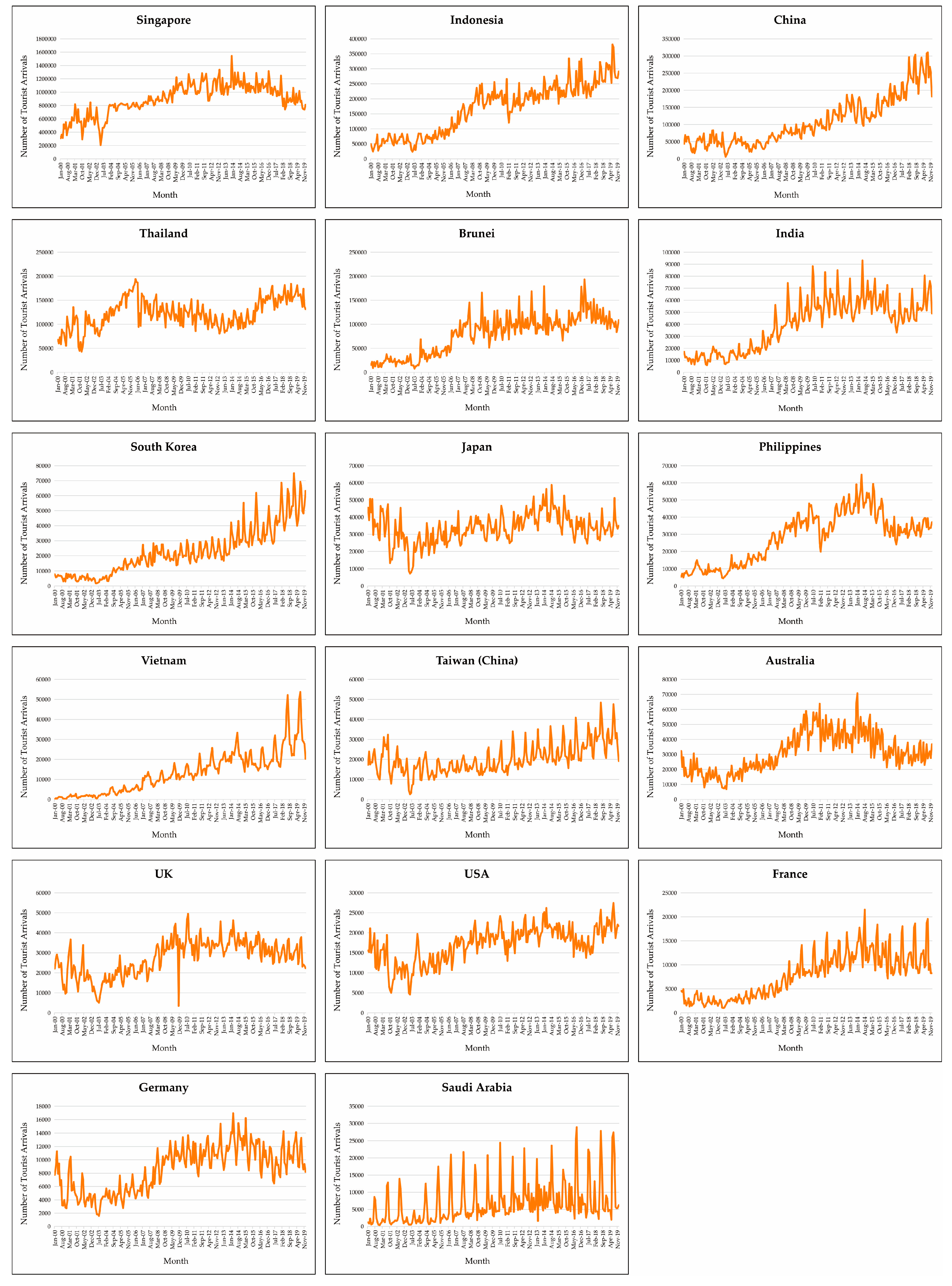
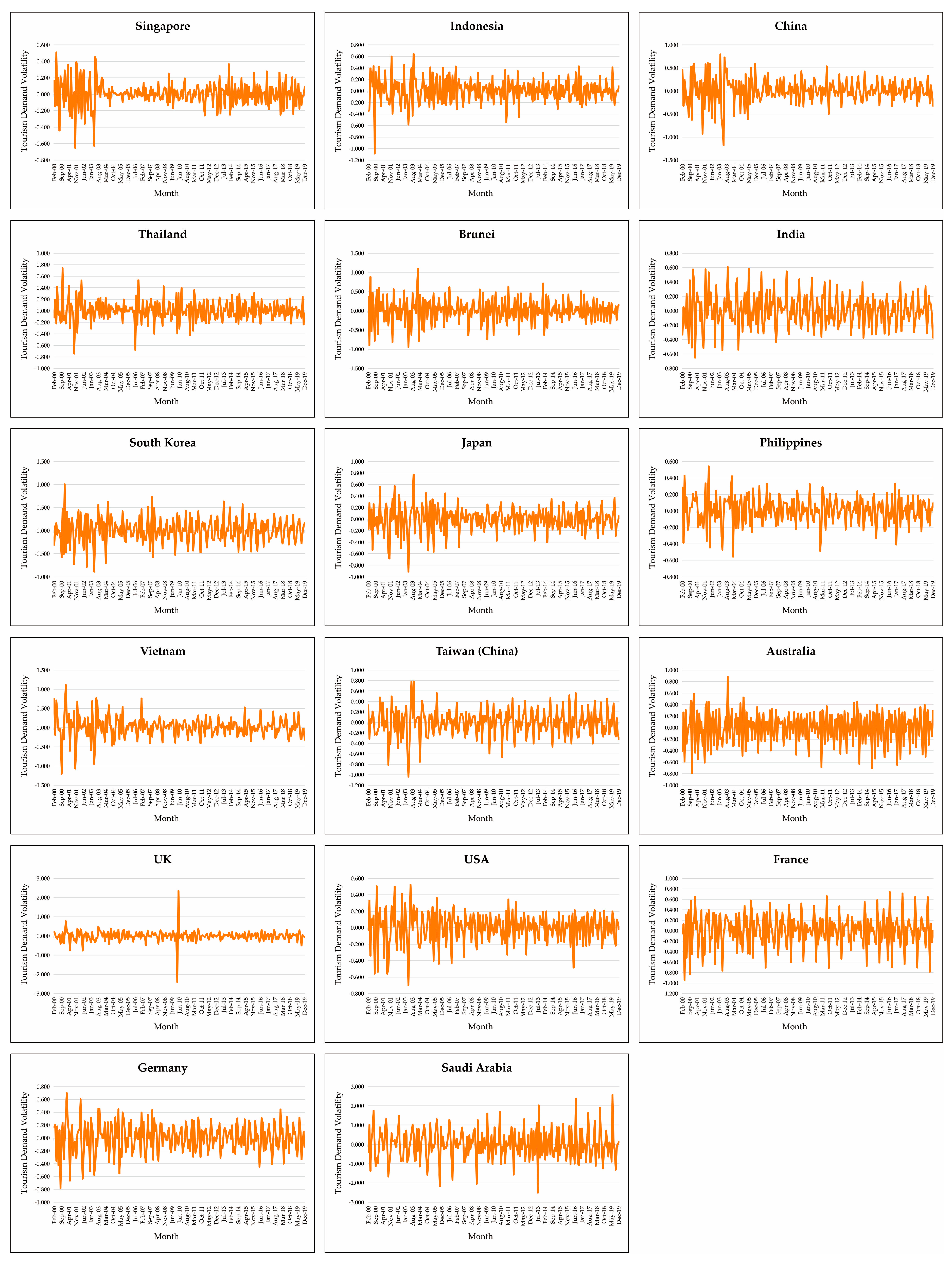
Based on AIC and BIC values, the first column of Table 4 displays the mean equations for various series. These models created “residuals” for variance equation modeling and forecast combining methods evaluation for forecasting the Malaysian tourism demand volatility. The unit root(s) and the requirement for differences, as determined by the ADF and PP tests, indicate that each series meets the associative significance criteria of at least 5%. Obviously, the models of China, Brunei, India, South Korea, and Australia have AR parameters. Importantly, these models provide seasonal parameters for all series. In this study, the relative order of seasonal and nonseasonal factors was established by combining Figure 1 and Figure 2. These certificates allow us to account for seasonality in the modeling process and analysis of news shocks.
Since several volatility models were used to examine seasonal volatility estimates for Malaysia tourist arrivals data, the conditional variance equation must always be discovered during the second phase. The completed SARIMA-conditional variance equations (GARCH, EGARCH, and GJRGARCH) suggest that tourism movements into Malaysia are volatile, and Table 5, Table 6 and Table 7 present additive seasonal patterns with variable amplitudes for inbound tourism statistics. The results are consistent with the prior findings [12,37,57,78,86,141]. This study utilized lag month values to assess monthly changes in Malaysian tourism demand. This is because the lagged dependent variables can reduce the occurrence of autocorrelation resulting from model misspecification. Consequently, we can defend the presence of autocorrelation in the model by taking lagged dependent variables into consideration. Importantly, months in different years are accompanied by sudden news shocks, such as natural disasters, disease, climate fluctuation, events, and financial crises, which will have gradual short-term or long-term delayed effects on incoming tourism. In other words, many visitors’ decisions or behaviors may be more sensitive to long-term changes in tourism circumstances or surroundings than they are to transient fluctuations in conditions. In this instance, the lagged values of conditions determine the duration of the change, and the presence of lagged effects illustrates this unequal reaction to short-term and long-term tourism variation. In addition, these data are monthly time series, and with the unique monthly dummy, the coefficients of each month t represent that month’s influence on the tourist arrivals of the following month (t + 1).
GARCH (1,1) models in Table 5 have an asterisk value to indicate that the model’s parameters are statistically significant at p values less than 10%, 5%, and 1%, respectively. In all series, the volatility of Malaysian tourism demand is more likely to be affected by news shocks since α + β equals 1. However, with only a few series having a large monthly impact (a significance at 10%, 5%, and 1% correspondingly), GARCH (1, 1) shows that the effect of tourism on each series is less pronounced. For example, according to the coefficients of months in different series, January (−1), February (−1), March (−1), July (−1), August (−1), and October (−1) in S1 (Singapore) have implications for tourists entering Malaysia; S3 (China) represents February (−1), May (−1) and October (−1); S5 (Brunei) shows January (−1), April (−1), May (−1), July (−1) to October (−1) and S13 (UK) displays May (−1), August (−1), and Nov (−1). Overall, in the GARCH (1,1) model, May, August, and October have a larger monthly impact on tourists.
However, the GARCH model is incapable of examining asymmetric effects and the influence of both positive and negative news shocks on leverage. GJRGARCH and EGARCH models were developed in response to this issue. In the EGARCH (1,1) models presented in Table 6, the coefficients ϕ that are highlighted with an asterisk indicate that they reach statistical significance at 1%, 5%, and 10%, respectively, including S1 (Singapore), S3 (China), S6 (India), S7 (South Korea), and S13 (UK). All of these values, with the exception of S6 (India), demonstrate that ϕ is less than zero, which suggests that leverage effects are presented in the models. In addition, the presence of a negative sign for shows that bad news has a higher impact on Malaysia’s monthly tourism demand volatility than good news. The EGARCH (1,1) model produced a greater monthly effect for visitors in all other series than the GARCH (1,1) model, with the exception of S15 (France). February (−1), May (−1), August (−1), October (−1), and November (−1) are the months that have the largest impact on Malaysian tourist arrivals.
While the leverage effect is being analysed, asymmetric GJRGARCH model allows the conditional variance to respond differentially to bad and good news. Referring to Table 7, there are the asymmetric effects on the monthly tourism demand volatility in the GJRGARCH (1,1) model, which are presented in S2 (Indonesia), S4 (Thailand), S5 (Brunei), S7 (South Korea), S8 (Japan), and S16 (Germany). At the same time, through the coefficients of months in different series, GJRGARCH (1, 1) modeling produces fewer monthly effects on inbound tourists to Malaysia compared to GARCH (1, 1) and EGARCH (1, 1). Only S3 (China), S4 (Thailand), S5 (Brunei), S9 (Philippines), S11 (Taiwan (China)), S13 (UK), S16 (Germany), and S17 (Saudi Arabia) have monthly effects.
The values for adjusted R2, log-likelihood, AIC, and BIC are used to analyze and investigate the conditional variance, which is determined based on the forecasting ability of each volatility model. In other words, the conditional variance is determined based on how well each model can forecast future volatility. The EGARCH (1,1) model has the highest adjusted R2 values and outperforms the GJRGARCH (1,1) and GARCH (1,1) models in log-likelihood performance. The AIC and BIC of EGARCH (1,1) is the lowest. Furthermore, the EGARCH (1,1) represents more monthly effects for the most series. Hence, it can be inferred that the EGARCH model utilized in this study had the most significant power to forecast conditional variance. Malaysian tourism developers can adjust tourism marketing strategies and plans accordingly based on EGARCH modeling and the dynamics of tourists in the lag few months.
In addition to the above-mentioned analysis, as an example, it relies upon the following selected criteria: (i). top tourist arrivals into Malaysia from different states/areas; (ii). top expenditures from different states/areas; (iii). the temperate countries/regions with distinct seasons; we chose the UK, the USA, China, Germany, and Australia, shown in Table 8, to compare the conditional variance equations. Table 8 depicts the estimated parameters for the conditional variance equations based on the three unique volatility models with the seasonal dummy, GARCH (1,1), GJRGARCH (1,1), and EGARCH (1,1), corresponding to the Table 4 mean equations for the five tourist arrival markets. It basically displays the model with the maximum log-likelihood (LL), adjusted R2, AIC, and BIC statistics when more than conditional variance equations have significant parameters while adhering to specified limits. In addition, dummy variables for the reference month, December, are calculated from JAN (January) to NOV (November).
Seasonal dummies are significant at p < 0.01 or p < 0.1, indicating that monthly seasonality occurs. The GARCH (1,1) model suggests that May (−1), August (−1) and November (−1) have monthly impacts on tourist arrivals from the UK. Similarly, the EGARCH (1,1) model shows May (−1), August (−1), October (−1), and November (−1) effects on visitor arrivals from the UK. All the remaining lag months have monthly influences on tourist arrivals from the UK, except February (−1), April (−1), June (−1), and July (−1). Therefore, under the influence of the lag months, there will be more British tourists traveling to Malaysia in June, September, and December. This is because the UK is mainly located in the northern part of Europe, and it enjoys a typical maritime climate with relatively minimal temperature changes between seasons and a lot of rain. Generally speaking, the months between June and September include public holidays in the UK. The weather in spring and autumn is changeable and humid, and the winter (November–February) is cold with little sunshine. Therefore, the British prefer to travel in summer.
As for the USA, GARCH (1,1), EGARCH (1,1), and GJRGARCH (1,1) models indicate no marked monthly impacts on tourist arrivals to Malaysia. Due to the vast territory and complex terrain of the USA, the weather varies greatly from place to place. However, most regions of the USA have a continental climate, but the south has a subtropical climate. There is a large temperature difference between the central part and northern plains. Meanwhile, like Malaysia, America is a multiracial country, and that is one reason why Malaysia attracts them. Thus, visitors from the USA travel abroad regardless of the season of the year, unaffected by any monthly effects.
In China, the GARCH (1,1) model reveals February (−1), May (−1), and October (−1) effects on tourist arrivals to Malaysia. All the remaining lag months, except January (−1), March (−1), June (−1), and August (−1), have monthly effects on tourist arrivals from China in the EGARCH (1,1) and GJRGARCH (1,1) models. The Chinese Spring Festival holiday is celebrated from January to February, the summer holiday lasts from June to August, and the National Day holiday falls in October. These holidays motivate seasonal traveling [142,143].
The monthly effect results of Germany are comparable to those of China. In the GJRGARCH (1,1), GARCH (1,1), and EGARCH (1,1) models, the effects of January (−1), February (−1), March (−1), April (−1), June (−1), September (−1), and November (−1) on tourist arrivals from Germany are notable. Germany is in a cool, westerly wind belt of the eastern Atlantic, having a continental climate. Extreme temperatures and sharp temperature fluctuations are rare here. It rains all year round. Spring in Germany (April–May) is relatively short and cold, with varied temperatures. Summer (June–August) is rainy and hot. Autumn (September–November) is warm and dry, and much rain falls. In winter (December–March), there is sufficient precipitation, and it is extremely wet and cold. Like China, Germany is a country with four distinct seasons. However, it is like summer all the year round in Malaysia. According to the above analysis, it is reasonable that Germans like to travel to Malaysia. In the meantime, there are cultural links in education and language between Germany and Malaysia. Besides, several German political foundations support sociocultural, education and media projects in Malaysia. These factors further facilitate tourism exchanges between the two countries.
Similar to the USA, there are almost no monthly effects on tourist arrivals from Australia to Malaysia. In the EGARCH (1,1) model, July (−1) and August (−1) effects on the number of tourists visiting Australia are remarkable. Located in the southern hemisphere, Australia has a tropical climate varying between desert and semi-desert. Most of the area of this country is arid. The seasons here are opposite to those in the northern hemisphere. Australia and Malaysia conduct cultural, economic, and trade exchanges. Thus, passengers from the USA may travel overseas at any time of year without being influenced by seasonal fluctuations.
Taken above, tourist arrivals to Malaysia from the USA and Australia are not affected by months. Visitor arrivals to Malaysia from the UK, China, and Germany are notably affected by months, according to the results of the three methods. An increasing number of tourists are inclined to travel to Malaysia for the reason that Malaysia is close to the equator and has a tropical rainforest climate and a tropical monsoon climate. There is no notable variation of the weather with the season, and the annual temperature remains almost unchanged. Malaysia is a multicultural country with various religions and cultural beliefs, so it is known as the best place to “experience the charm of Asia”. Coming to Malaysia, tourists can learn about three major Asian civilizations, namely Malay, Chinese, and Indian cultures. Moreover, the pace of life in this country is slow and people here live a life of leisure and ease. The unique landscape and the summer-like weather all the year around make Malaysia a tourist attraction, luring an average greater than tens of millions of global tourists every year.
While forecast evaluation is the primary objective of this work, it is fascinating to observe how well the GARCH (1,1), GJRGARCH (1,1), and EGARCH (1,1) models read statistical measures of tourism demand volatility and how news shocks influence key source tourist arrivals separately. The GARCH (1,1) model is symmetric, so it cannot accurately capture leverage or asymmetric effects. The essential ϕ of the EGARCH (1,1) model and γ of the GJRGARCH (1,1) model are significant at p < 0.01 or p < 0.1, demonstrating that asymmetric or leverage effects respond to shocks of tourist arrival news. In the EGARCH (1,1) model, the ϕ values of the UK and China are less than zero, indicating that the tourism demand volatility is affected by a negative shock of “bad news”. Meanwhile, only the γ value of Germany is significant and greater than zero, suggesting that the GJRGARCH (1, 1) model has leverage effects on tourists to Malaysia from Germany.
Therefore, as for these many models, the magnitude and duration of unstable oscillations in tourism vary depending on the type of shocks the destination experienced. As demonstrated by the preceding examples, the GJRGARCH (1,1) model forecasted strong positive shocks for Germany. According to the EGARCH (1,1) model, powerful negative shocks increase the volatility of tourist arrivals in Malaysia more than positive shocks of the same magnitude, but only within the selected series.
Moreover, asymmetries and symmetries in the impacts on visitors are the topic of models, such as GARCH (1,1), EGARCH (1,1), and GJRGARCH (1,1), based on the study of the preceding models. Consequently, as a specific illustration, Figure 4 depicts the estimated conditional variance under the impacts of news shocks up to December 2014 for four analyzed series: China, Japan, the USA, and Australia. This is because news shocks have direct and indirect effects on tourism demand. Current events may influence the desire for tourism. The graph illustrates that the four series experienced the similar period of SARS spread volatility in 2003. Due to the tremors of a 7.0 magnitude earthquake that struck the main island in May and an 8.3 magnitude earthquake that struck in September 2003, Japan became very volatile in 2003. In 2001, the USA’s response to the shocks of September 11th was comparatively volatile. Other volatile periods following them for Australia are the 2000 summer Olympics ending with a big party in October 2000, the flooding crisis in February 2011, and lightning strikes that ignited fires in January 2014. However, other periods reacted in a less volatile manner to shocks [144,145,146,147,148,149,150,151,152]. Therefore, whether an internal or external news shock occurs in a country/region may influence on the inbound or outgoing tourism of tourists.
The next step is to construct the exponential smoothing models. When computing the exponential smoothing values for every interval, the weighted average of the current period’s observations and the historical exponential smoothing values serve as the basis for computation. Depending on Table 1 and Table 2, using the AIC and BIC, the best, most distinct ETS-ES models derived for each series with incoming tourist arrivals to Malaysia were determined via EViews 11 in Table 9. As demonstrated in Table 9, the smoothing procedure can be applied outside the context, including its in-sample data, to generate out-of-sample smoothing forecasts of the array. The higher value of parameter α indicates that the model focuses on even the most recent historical observations. In comparison, the lower value implies that the model considers much of the past while conducting a forecast. β regulates the dampening degree at which the effect of a pattern shift declines. The method is compatible with patterns that vary in two different ways (additive and multiplicative) and focuses on whether the pattern is linear or exponential. Similar methods were utilized to reduce the propensity to represent it explicitly, additively or multiplicatively for a linear or exponential decay impact. China, the Philippines, Vietnam, and Saudi Arabia are examples of series where the slope of a series has stayed strikingly consistent across time. The models from China, Thailand, and Brunei have used a damping coefficient, ϕ, to manage the decay rate. γ restricts the effect on the seasonal factor. The values of γ are very large, demonstrating that the series is greatly influenced by seasonality. Eleven series’ ETS-ES models (China, India, South Korea, Japan, the Philippines, Taiwan (China), Australia, the UK, the USA, Germany and Saudi Arabia) for international tourist arrivals are subject to seasonality, with the UK having the most significant seasonality. Singapore, Indonesia, Thailand, Brunei, Vietnam, and France have not developed any seasonality models.

6. Empirical Results of Out-of-Sample Volatility Forecasting Accuracy

Before integrating all models of volatility, this research must determine the best single model based on several evaluation criteria. Taylor (2004) stated in [23,24] that the GJRGARCH (1,1) estimation outperforms the GARCH estimation in data processing. Here, our benchmark model of choice would be GJRGARCH for the further data processing. Importantly, Theil-U statistics is specified as the ratios of the MAE, MSE, RMSE, and MAAPE inside GJRGARCH forecasting to the MAE, MSE, RMSE, and MAAPE within our forecasting models. To determine which model is the most accurate, we calculated the values of mean Theil-U statistics for the whole series in the final column of Table 10, Table 11, Table 12, Table 13, Table 14 and Table 15. The value of U-statistics just below one indicates vastly superior performance with a comparison to the GJRGARCH. In other words, the lower the value, the better the model [23,24,153].
A total of nine different SARIMA-GARCH and SARIMA-ES family models were examined for this study, and the results are listed in Table 10. First, to determine whether the results of this study can adequately address the questions posed by the objectives, we need to select the best model to combine from each relevant family. Therefore, these nine models were estimated using four evaluation criteria (MAE, MSE, RMSE, and MAAPE) for each of the 17 series. After that, we determined the best single model to combine by computing the mean rank of all mean Theil-U values under evaluation criteria between two-family methods. STES-AE (0.854), ETS-ES (0.887), and EGARCH (0.903) are the models that have the lowest values in MAE; the best models in terms of both MSE and RMSE are STES-E (0.742, 0.853), ETS-ES (0.912, 0.860), and GJRGARCH (1.000, 1.000), separately; MAAPE with the fewest values are EGARCH (0.926), STES-ESE (0.958), and ETS-ES (0.969). It is regarded as fair to use the mean rank to determine which model is the best because the best model may not always be the same for each evaluation criterion. Consequently, based on the final mean rank in Table 10, the best STES model is STES-E, followed by the ETS-ES model from the ES family. Similarly, GJRGARCH is a superior model within the GARCH family, but it ranks behind the other two. The results confirm unequivocally the consistency discovered by Coshall (2009) in [9], where exponential smoothing combining models outperform volatility models. Therefore, STES-E, ETS-ES, and GJRGARCH were utilized to test if the forecast combining methods outperform the single forecasts methods during the process of combining.
To determine whether our suggested novel methods can increase the accuracy of tourism demand volatility forecasting in Malaysia, we presented multiple evaluation criteria (MAE, MSE, RMSE, MAAPE, R2, MCS test, and DM test). The highlighted values indicate the optimal model. In the meantime, the prior methods are used independently to produce monthly estimates for the out-of-sample absolute forecasting error and squared forecasting error in the combining phase for 17 tourist arrivals time series. Consequently, the data from January 2015 to December 2019 were used to illustrate the forecasting performance of several methods in this subsection. The forecast was generated by combining the results of SA, MV, and ST (ST1 (sign of residuals), ST2 (size of residuals), ST3 (absolute (residuals)), ST4 (sign of residuals + size of residuals), ST5 (sign of residuals + absolute (residuals)), and ST6 (size of residuals + absolute (residuals))), spanning Table 11, Table 12, Table 13, Table 14, Table 15, Table 16, Table 17, Table 18 and Table 19. Overall, the top five forecast combining models are denoted in bold in the last column for each respective series.
The comparison of single models and forecast combining methods in Table 11, Table 12, Table 13, Table 14, Table 15, Table 16, Table 17, Table 18 and Table 19 reveals that the average forecasting performance of ES family models (M1, M2) is superior to that of GARCH family models (M3, M4, M5) for forecasting the Malaysian tourism demand volatility. The forecasting performance of STES-E is marginally superior to that of ETS-ES. At the same time, the average forecasting performance of single models overall is lower than the performance of forecast combining methods based on MAE, MSE, RMSE, MAAPE, R2, MCS test, and DM test. ETS-ES and EGARCH offer superior forecasting performance compared to MAAPE. In addition, ES family methods have improved forecasting performance in the R2 and DM tests, particularly STES-E. These results indicate that the forecasting performance of the best single model can surpass that of forecast combining methods. However, the performance of the poorest single model cannot. In other words, forecast combining methods are not necessarily the best models for forecasting tourism demand volatility.
The rank of mean Theil-U results in the SA combining method in MAE, MSE, RMSE, MAAPE, R2, MCS test, and DM tests indicate that all combining models outperform the worst single model. While SA is acknowledged in the financial sector, the results indicate that the SA forecast combining method has the smallest sums among the top five forecast combining models in each series from Table 11, Table 12, Table 13, Table 14, Table 15, Table 16, Table 17, Table 18 and Table 19, except for MAE. The superiority of the forecast combining methods under the SA combining method is barely discernible in comparison to the other models examined in this study. This demonstrates that the SA combining method is not optimal for creating the combining models in the tourism demand volatility forecasting of this study. In the meantime, the combining weights for the minimum variance (MV) forecast combining method are computed, and the preceding performance of the forecast combining methods is considered throughout Equation (9). Excel’s “Solver” function can provide ideal weights for the minimum variance equation in various combining models to produce the best values across all evaluative criteria. All forecasting evaluation criteria indicate that MV’s average forecasting performance is substantially inferior to other forecast combining methods. However, it is superior to single models. In general, the SA combining method is not more prominent than other combining methods in the 17 series. Similarly, MV is still not the optimal method for forecasting the Malaysia’s tourism demand volatility. The outcomes transcend the conclusion reached by Shen et al. (2011) in [30], that the minimum variance forecast combining method was the most effective in combining research. The results of the mean Theil-U indicate that, except for the STES-E and ETS-ES models, forecast combining does not consistently outperform the best single forecast. The combining outcomes of SA and MV are coincidental with the results of Andrawis et al. (2011) in [154], Jun et al. (2018) in [155], Winkler and Clemen (1992) in [156], and Wong et al. (2007) in [27]. This is because the weight values assigned to one of the other models affect the forecast combining results. This appears to be another reason why forecast combining does not routinely improve forecasting performance over single forecasts.
The empirical results are currently being reconsidered from a new angle. From Table 11, Table 12, Table 13, Table 14, Table 15, Table 16, Table 17, Table 18 and Table 19, it is evident that combining estimates from multiple distinct models tends to prevent the worst forecasts. Clearly, the smooth transition (ST) combining method produces favorable results for forecasting the inbound tourism demand volatility in 17 source markets in Malaysia. Similarly, the ST combining method must utilize the “Solver” to automatically determine the appropriate weight for the transition variable in Equation (11) to obtain the best combining method based on all evaluation criteria. Therefore, whether under ST1, ST2, ST3, ST4, ST5, or ST6, there is a top five combining methods cluster in different series to be obtained via the MAE, MSE, RMSE, MAAPE, R2, MCS test, and DM test. Therefore, the average performance of the ST method exceeds that of the other methods. Significantly, based on the rank value of mean Theil-U across single models, the top five combining methods are all included in distinct series of the ST combining method. The top five forecast combining methods are denoted with a bold underline. This demonstrates that the relative forecasting output by the combining methods versus the single models vary by countries/regions of origin. In addition, the results reveal that, among 16 forecast combining methods in each of main three forecast combining methods, the average performance of STES-E_GJRGARCH exceeds that of ETS-ES_GJRGARCH across all evaluation criteria. The MCS and DM tests significantly confirm the results of the evaluation criteria. Among them, the best models are the M11 and M15, followed by M13, M17, and M21. They are all STES-E_GJRGARCH methods in ST. Importantly, their average performance of forecast combining surpasses that of the best single forecast model. According to the literature, GJRGARCH is the best model, while STES is the most novel method. Thus, the performance of ST2 and ST4 with STES-E_GJR is superior to that of other ST combining methods based on various evaluation criteria. This is because ST accounts for all optimization transition factors, including sign and size. This method permits the combining to adapt over time to the relative supremacy of the single models. In other words, by matching the optimal parameters, ST can reduce the error in forecasting of the combining models.
For the series included in this study, it is evident that combining ST forecasts with SA and MV improves forecasting accuracy. Therefore, in many instances, the ST combining method is a worthwhile procedure for the forecast combining of tourism demand volatility. In addition, the study indicated that forecast combining does not always outperform the best single model but provides more accurate forecasting than the worst single model, depending on the source markets evaluated and the combining methods utilized.
As represented in the forecasting methods subsection, we employed the MCS test of Hansen et al. (2011) in [130]. This was conducted to determine if the prior statistical results are statistically accurate. The objective here is to increase the predictability of forecast combining while optimizing the post-processing of forecast combining methods. The R software provides the “MCS test package” to evaluate the significance of combining methods and produce forecasts with a high degree of precision. The absolute squared error was utilized to assess the effectiveness of single and forecast combining methods. If the method is superior to other methods, 1 is used to indicate this; otherwise, 0. They were used to calculate the total counts of the 17 series. We used the counts to determine if the MCS test findings support the prior MAE, MSE, RMSE, MAAPE, R2, and Theil-U results.
The different entries in each column of Table 16 and Table 17 show the number of methods that adhered to the SSM during the MCS test procedure, categorized by model. Using squared forecast error and absolute forecast error, we find that the SSM becomes very uniform in terms of its models’ shapes. As measured by MCS, it can be seen that the performance of the combining models is superior to that of the single models. Overall, the MCS test suggests that ETS-ES and STES-E are the most accurate single forecasts, even surpassing other forecast combining methods. This again demonstrates that the best single forecasts methods outperform the weakest forecast combining methods. However, the GARCH family models have the weakest forecasting performance, followed by the SA and MV forecast combining methods. Significantly, ST performed in a fiercely competitive manner, with STES-E yielding the best results for all methods. Consequently, based on the results of squared forecast error and absolute forecast error, the methods with STES-E are the least excluded models among those utilized in this research. Simultaneously, the combining methods with the greatest number of counts continue to employ the ST combining methods, namely STES-E_GJRGARCH (M11, M13, M15, M17, and M21) with 14 counts and squared forecast error. These outcomes support the primary MSE and RMSE evaluation criteria outcomes. ETS-ES_GJRGARCH (M10, M18, and M20) and STES-E_GJRGARCH (M13, M15, and M21) with the most, namely ten, counts utilize the ST combining method employing absolute forecast error. The SA and MV combining methods yield the poorest outcomes overall. Consequently, the ST forecast combining method is preferable, which is consistent with the findings of the aforementioned criteria.
Diebold and Mariano (2002) in [133] used the loss-differential test to test the null hypothesis that two forecasts possess identical forecasting accuracy. The DM test was performed by building the t statistics with a simple regression of the loss function based on a constant using a Newey–West estimator for MAE and RMSE. A negative sign for the t-statistic associated with the DM test shows that the forecast error connected with the competitive series forecast is reduced, whereas a positive sign implies the opposite. Therefore, when comparing the two models based on t statistics, we employed “1” to indicate that the benchmark model makes more accurate forecasts than the other volatility model in each comparison for every series, and “0” to indicate that the two models have the same forecasting accuracy in this study. After calculating the results of the comparison between the two models in 17 series, it is determined that the model with the highest number of “1” is the best model for forecasting Malaysian tourism demand volatility. This further verifies whether the joint forecast models can outperform the single models.
In addition, Table 18 and Table 19 display the evaluated values of the DM test for the out-of-sample performance of a total of 21 methods. These tables compared methods’ differentials from MAE and RMSE in 17 series using the “row versus column” format. The null hypothesis was tested without changes in forecasting accuracy. Most DM test results reject the null hypothesis that the forecasting error of the benchmark modes are equivalent to either of the comparison models. The comparison’s results are separated into two portions for analysis. First, compare the forecast combining methods to the single models. The MAE results indicate that the forecast combining methods, particularly the ST forecast combining method, produces statistically superior results compared to methods 3 and 4. Similarly, in terms of RMSE, ST achieves superior statistics when comparing forecast combining methods using SARIMA-GARCH family models as benchmarks. In contrast to ES family models (ETS-ES and STES), however, forecast combining methods produce fewer statistics for MAE and RMSE. Second, when compared to the SA and MV forecast combining methods, ST produces comparatively more statistics overall, when ST is compared as the standard to method 9. Nonetheless, when comparing ST to its own family methods, several results do not reject the null hypothesis. DM test results are consistent with earlier criteria (MAE, MSE, RMSE, and MAAPE).
All aforementioned findings indicate that the forecasting performance of ES family models exceeds that of GARCH family models. In the meanwhile, the forecast combining does not always outperform the best single forecasts, but nearly outperforms the worst single forecast. Among the forecast combining models that outperform single models, ST is the best forecast combining method for forecasting Malaysian tourism demand volatility. This indicates that forecast combining can greatly reduce the probability of an incorrect forecast. In many real-world settings, it follows that forecast combining is superior to single forecasts.

7. Conclusions

This is one of the few studies to incorporate modeling volatility forecast combining within the context of tourism volatility and to primarily evaluate the forecasting potential of this class of model. In this work, the empirical results of single and combining methods for forecasting tourism demand volatility are explored further. The primary purpose is to determine whether forecast combining outperforms single forecasts and whether forecast combining can improve forecasting accuracy when utilizing the ST forecast combining method. Single forecasts, such as ETS-ES, STES-E, GARCH, EGARCH, and GJRGARCH, were utilized to investigate this phenomenon. Moreover, if two forecasts offer overlapping information, forecast merging is unlikely to outperform the forecasts offered by each model individually. Forecast combining will only be effective when forecast error correlations between single forecasts are minimal. Therefore, we utilized SA, MV, and a recently proposed ST for combining volatility forecasts.
This study reveals that, among the GARCH-type family models, the GJRGARCH model is superior. In out-of-sample tourism demand volatility forecasting, STES fared best among the single models, followed by ETS-ES. Intriguingly, forecast combining methods do not always outperform the best single model, but they do outperform the worst single model. The ST combining method surpasses the SA and MV methods. It is an effective method for making accurate forecasts despite the tourism demand volatility. This is because ST accounts for the necessary optimization transition factors, such as sign and size. This method permits the combination to adjust over time to the relative superiority of the different methods by modeling the combining weight as a logistic function of one or more transition factors. In other words, once ST matches the most relevant parameters to discover the shortest forecasting error, this can lower the forecasting error of the combined models, resulting in the best model. ST has been discovered to be the best method for combining volatility forecasts across all forecast combining models. Consequently, by evaluating the performance of various volatility forecast combining methods, we provide support to the assertion that forecasts are more accurate and dependable when employing the ST forecast combining method.
Significantly, the MCS test and DM test increase the confidence of the aforementioned forecasting results, making it necessary to execute these tests by combining single models. This is a novel solution to the problem of determining the “best” forecasting method among volatility forecast combining methods, based on the MCS, employing a out-of-sample evaluation beneath a loss function proposed in this study. It is straightforward to evaluate whether the forecast combining outperforms the single forecasts by using the MCS test to the ensemble of models, with the forecast combining as an additional model. In the meantime, DM loss-differential forecasting accuracy testing examines the particulars and distinctions between two competing series. Therefore, it can bolster the competitive comparison between the two forecasting models evaluated in this article.
In terms of tourist arrivals assessments, substantial volatility models of 17 tourist arrivals into Malaysia have been built, which are likely to be of greater actual value. The conditional variance and tourist arrivals over time revealed the volatility associated with negative shocks, such as the SARS outbreak in 2003 and the September 11th, 2001 tragedy. Both of these periods influenced the influx of tourists from many countries/regions into Malaysia. Additionally, periods of volatility were typically brief. The models demonstrated that the magnitude and duration of tourism demand volatility vary depending on the nature and location of shocks. Negative shocks had a greater influence on tourism demand volatility at the sites investigated than positive shocks of equal magnitude. The tourism product might not be as fragile as is generally believed. Integrated with an exponential smoothing time series model, the advantage of modeling volatility is revealed when forecasting the tourism demand volatility.
The findings of this study have significant implications for the tourism industry and government agencies. First, for tourism-related businesses to minimize losses caused by an imbalance between the supply and demand for tourism goods and services, accurate forecasts of tourism demand volatility are essential. This is related to effective management and sound decisions considering investments in different tourism facilities and project expansion. When faced with several sets of forecasts generated by diverse models, certain business executives may become overwhelmed. Their most reliable option is based on combining the best single forecasts, but they instead choose those generated from the weakest single model. If forecasting swings in tourism demand can be improved by integrating the best single and forecast combining, then tourism policy decision-makers in both the public and private sectors will certainly value this. Based on the general extent and independent resource marketplaces, applicable administrative tourist rules and competitive business strategies of destination marketing agencies will aid in forecasting the expansion and trends of tourism volatility.
This study makes a substantial contribution to either specific or tourism volatility forecast combining studies by offering findings on the productivity of forecast combining. In the future, it would be worthwhile to examine other transition variables, like macroeconomic variables. It would also be interesting to see the outcomes of combining ST with other data and forecasting methods. As ST permits the combining weights to adjust gradually and smoothly over time as relevant transition variables adapt, we plan to examine its performance over a somewhat longer time series in future research. Another extension of our investigation would be to explore an ST that combines more than two single models. In addition, significant research into advanced and specialized volatility forecast combining methods, as well as newer linear or non-linear combining methods, is forecasted. This should also be assessed to determine if these methods provide a more accurate combination of tourism demand volatility forecasts than those offered in the tourism demand volatility forecasting sector.

Author Contributions

Conceptualisation Y.Z. and W.C.C.; formal analysis and methodology, Y.Z., W.C.C., and J.S.H.; wring—original draft, Y.Z.; projection administration, W.C.C.; visualisation, W.C.C. and C.K.W.; wring—review and editing, C.K.W. and J.S.H. All authors have read and agreed to the published version of the manuscript.

Funding

This research received no external funding.

Institutional Review Board Statement

Not applicable.

Informed Consent Statement

Not applicable.

Data Availability Statement

The data used to support the findings of this study are included within the text.

Acknowledgments

The authors would like to thank the “RightsLink”, “Copyright Clearance Center, Inc.”, and “Elsevier”, which provided the copyright licenses for adapted or cited tables in this research. The authors are also grateful to “Bergmeir, C.; Hyndman, R. J.; Benítez, J. M. Bagging exponential smoothing methods using STL decomposition and Box–Cox transformation. Int. J. Forecast. 2016, 32, 303-312.” for providing Table 2 copyright permission. The authors would like to thank the Ministry of Tourism, Arts and Culture of Malaysia for providing data on this work. The authors would also like to appreciate the editors and anonymous reviewers for their helpful and constructive comments.

Conflicts of Interest

The authors declare no conflict of interest.

References

  1. Li, C.; Ge, P.; Liu, Z.; Zheng, W. Forecasting tourist arrivals using denoising and potential factors. Ann. Tour. Res. 2020, 83, 102943. [Google Scholar] [CrossRef]
  2. UNWTO. Tourism—An Economic and Social Phenomenon. 2019. Available online: https://www.unwto.org/why-tourism (accessed on 18 June 2022).
  3. Jiao, X.; Li, G.; Chen, J.L. Forecasting international tourism demand: A local spatiotemporal model. Ann. Tour. Res. 2020, 83, 102937. [Google Scholar] [CrossRef]
  4. Kim, S.S.; Wong, K.K. Effects of news shock on inbound tourist demand volatility in Korea. J. Travel Res. 2006, 44, 457–466. [Google Scholar] [CrossRef]
  5. Li, G.; Song, H.; Witt, S.F. Recent developments in econometric modeling and forecasting. J. Travel Res. 2005, 44, 82–99. [Google Scholar] [CrossRef] [Green Version]
  6. Palmer, A.; Montano, J.J.; Sesé, A. Designing an artificial neural network for forecasting tourism time series. Tour. Manag. 2006, 27, 781–790. [Google Scholar] [CrossRef]
  7. Xie, G.; Qian, Y.; Wang, S. A decomposition-ensemble approach for tourism forecasting. Ann. Tour. Res. 2020, 81, 102891. [Google Scholar] [CrossRef]
  8. Jiang, P.; Yang, H.; Li, R.; Li, C. Inbound tourism demand forecasting framework based on fuzzy time series and advanced optimization algorithm. Appl. Soft Comput. 2020, 92, 106320. [Google Scholar] [CrossRef]
  9. Coshall, J.T. Combining volatility and smoothing forecasts of UK demand for international tourism. Tour. Manag. 2009, 30, 495–511. [Google Scholar] [CrossRef]
  10. Song, H.; Qiu, R.T.; Park, J. A review of research on tourism demand forecasting: Launching the Annals of Tourism Research Curated Collection on tourism demand forecasting. Ann. Tour. Res. 2019, 75, 338–362. [Google Scholar] [CrossRef]
  11. Li, H.; Goh, C.; Hung, K.; Chen, J.L. Relative climate index and its effect on seasonal tourism demand. J. Travel Res. 2018, 57, 178–192. [Google Scholar] [CrossRef]
  12. Goh, C.; Law, R. Modeling and forecasting tourism demand for arrivals with stochastic nonstationary seasonality and intervention. Tour. Manag. 2002, 23, 499–510. [Google Scholar] [CrossRef]
  13. Rosselló, J.; Becken, S.; Santana-Gallego, M. The effects of natural disasters on international tourism: A global analysis. Tour. Manag. 2020, 79, 104080. [Google Scholar] [CrossRef]
  14. Song, H.; Livat, F.; Ye, S. Effects of terrorist attacks on tourist flows to France: Is wine tourism a substitute for urban tourism? J. Destin. Mark. Manag. 2019, 14, 100385. [Google Scholar] [CrossRef]
  15. Dergiades, T.; Mavragani, E.; Pan, B. Google Trends and tourists’ arrivals: Emerging biases and proposed corrections. Tour. Manag. 2018, 66, 108–120. [Google Scholar] [CrossRef]
  16. Shahrabi, J.; Hadavandi, E.; Asadi, S. Developing a hybrid intelligent model for forecasting problems: Case study of tourism demand time series. Knowl. -Based Syst. 2013, 43, 112–122. [Google Scholar] [CrossRef]
  17. Shen, S.; Li, G.; Song, H. An assessment of combining tourism demand forecasts over different time horizons. J. Travel Res. 2008, 47, 197–207. [Google Scholar] [CrossRef] [Green Version]
  18. Yu, G.; Schwartz, Z. Forecasting short time-series tourism demand with artificial intelligence models. J. Travel Res. 2006, 45, 194–203. [Google Scholar] [CrossRef]
  19. Jun, W.; Yuyan, L.; Lingyu, T.; Peng, G. Modeling a combined forecast algorithm based on sequence patterns and near characteristics: An application for tourism demand forecasting. Chaos Solitons Fractals 2018, 108, 136–147. [Google Scholar] [CrossRef]
  20. dos Santos Coelho, L.; Santos, A.A. A RBF neural network model with GARCH errors: Application to electricity price forecasting. Electr. Power Syst. Res. 2011, 81, 74–83. [Google Scholar] [CrossRef]
  21. Xu, S.; Chan, H.K.; Zhang, T. Forecasting the demand of the aviation industry using hybrid time series SARIMA-SVR approach. Transp. Res. Part E Logist. Transp. Rev. 2019, 122, 169–180. [Google Scholar] [CrossRef]
  22. Saranj, A.; Zolfaghari, M. The electricity consumption forecast: Adopting a hybrid approach by deep learning and ARIMAX-GARCH models. Energy Rep. 2022, 8, 7657–7679. [Google Scholar] [CrossRef]
  23. Taylor, J.W. Smooth transition exponential smoothing. J. Forecast. 2004, 23, 385–394. [Google Scholar] [CrossRef] [Green Version]
  24. Taylor, J.W. Volatility forecasting with smooth transition exponential smoothing. Int. J. Forecast. 2004, 20, 273–286. [Google Scholar] [CrossRef]
  25. Liu, M.; Taylor, J.W.; Choo, W.C. Further empirical evidence on the forecasting of volatility with smooth transition exponential smoothing. Econ. Model. 2020, 93, 651–659. [Google Scholar] [CrossRef]
  26. Kin, W.C.; Chong, C.W.; Nassir, A.M.; Habibullah, M.S.; Yusop, Z. Volatility Forecasting Performance of Smooth Transition Exponential Smoothing Method: Evidence from Mutual Fund Indices in Malaysia. Asian Econ. Financ. Rev. 2021, 11, 829–859. [Google Scholar] [CrossRef]
  27. Wong, K.K.; Song, H.; Witt, S.F.; Wu, D.C. Tourism forecasting: To combine or not to combine? Tour. Manag. 2007, 28, 1068–1078. [Google Scholar] [CrossRef] [Green Version]
  28. Li, G.; Wu, D.C.; Zhou, M.; Liu, A. The combination of interval forecasts in tourism. Ann. Tour. Res. 2019, 75, 363–378. [Google Scholar] [CrossRef]
  29. Taylor, J.W. Forecast combinations for value at risk and expected shortfall. Int. J. Forecast. 2020, 36, 428–441. [Google Scholar] [CrossRef]
  30. Shen, S.; Li, G.; Song, H. Combination forecasts of international tourism demand. Ann. Tour. Res. 2011, 38, 72–89. [Google Scholar] [CrossRef]
  31. Song, H.; Witt, S.F.; Wong, K.F.; Wu, D.C. An empirical study of forecast combination in tourism. J. Hosp. Tour. Res. 2009, 33, 3–29. [Google Scholar] [CrossRef] [Green Version]
  32. Croce, V. Can tourism confidence index improve tourism demand forecasts? J. Tour. Futures 2016, 2, 6–21. [Google Scholar] [CrossRef] [Green Version]
  33. Gunter, U. Improving Hotel Room Demand Forecasts for Vienna across Hotel Classes and Forecast Horizons: Single Models and Combination Techniques Based on Encompassing Tests. Forecasting 2021, 3, 884–919. [Google Scholar] [CrossRef]
  34. Gunter, U.; Önder, I. Forecasting city arrivals with Google Analytics. Ann. Tour. Res. 2016, 61, 199–212. [Google Scholar] [CrossRef]
  35. Gunter, U.; Önder, I.; Smeral, E. Are Combined Tourism Forecasts Better at Minimizing Forecasting Errors? Forecasting 2020, 2, 211–229. [Google Scholar] [CrossRef]
  36. Chan, C.K.; Witt, S.F.; Lee, Y.C.E.; Song, H. Tourism forecast combination using the CUSUM technique. Tour. Manag. 2010, 31, 891–897. [Google Scholar] [CrossRef]
  37. Coshall, J.T.; Charlesworth, R. A management orientated approach to combination forecasting of tourism demand. Tour. Manag. 2011, 32, 759–769. [Google Scholar] [CrossRef]
  38. Liu, L. Demand forecast of regional tourism based on variable weight combination model. In Proceedings of the International Conference on Information Computing and Applications, Chengde, China, 14–16 September 2012; pp. 665–670. [Google Scholar]
  39. Ma, X. Tourism Demand Forecasting Based on Grey Model and BP Neural Network. Complexity 2021, 2021, 5528383. [Google Scholar] [CrossRef]
  40. Wan, S.K.; Song, H. Forecasting turning points in tourism growth. Ann. Tour. Res. 2018, 72, 156–167. [Google Scholar] [CrossRef]
  41. Chen, K.Y. Combining linear and nonlinear model in forecasting tourism demand. Expert Syst. Appl. 2011, 38, 10368–10376. [Google Scholar] [CrossRef]
  42. Lütkepohl, H.; Netšunajev, A. Structural vector autoregressions with smooth transition in variances. J. Econ. Dyn. Control 2017, 84, 43–57. [Google Scholar] [CrossRef]
  43. Balli, H.O.; Tsui, W.H.K.; Balli, F. Modelling the volatility of international visitor arrivals to New Zealand. J. Air Transp. Manag. 2019, 75, 204–214. [Google Scholar] [CrossRef]
  44. Athanasopoulos, G.; Hyndman, R.J.; Song, H.; Wu, D.C. The tourism forecasting competition. Int. J. Forecast. 2011, 27, 822–844. [Google Scholar] [CrossRef]
  45. Jiao, E.X.; Chen, J.L. Tourism forecasting: A review of methodological developments over the last decade. Tour. Econ. 2019, 25, 469–492. [Google Scholar] [CrossRef]
  46. Athanasopoulos, G.; Song, H.; Sun, J.A. Bagging in tourism demand modeling and forecasting. J. Travel Res. 2018, 57, 52–68. [Google Scholar] [CrossRef]
  47. Song, H.; Witt, S.F.; Jensen, T.C. Tourism forecasting: Accuracy of alternative econometric models. Int. J. Forecast. 2003, 19, 123–141. [Google Scholar] [CrossRef]
  48. Wu, D.C.; Song, H.; Shen, S. New developments in tourism and hotel demand modeling and forecasting. Int. J. Contemp. Hosp. Manag. 2017, 29, 507–529. [Google Scholar] [CrossRef]
  49. Chan, F.; Lim, C.; McAleer, M. Modelling multivariate international tourism demand and volatility. Tour. Manag. 2005, 26, 459–471. [Google Scholar] [CrossRef]
  50. Chang, C.L. Modelling a latent daily tourism financial conditions index. Int. Rev. Econ. Financ. 2015, 40, 113–126. [Google Scholar] [CrossRef] [Green Version]
  51. Chang, C.L.; Hsu, H.K.; McAleer, M. The impact of China on stock returns and volatility in the Taiwan tourism industry. N. Am. J. Econ. Financ. 2014, 29, 381–401. [Google Scholar] [CrossRef] [Green Version]
  52. Chang, C.L.; Khamkaew, T.; Tansuchat, R.; McAleer, M. Interdependence of international tourism demand and volatility in leading ASEAN destinations. Tour. Econ. 2011, 17, 481–507. [Google Scholar] [CrossRef] [Green Version]
  53. Chikobvu, D.; Makoni, T. Statistical modelling of Zimbabwe’s international tourist arrivals using both symmetric and asymmetric volatility models. J. Econ. Financ. Sci. 2019, 12, a426. [Google Scholar] [CrossRef]
  54. Cho, V. A comparison of three different approaches to tourist arrival forecasting. Tour. Manag. 2003, 24, 323–330. [Google Scholar] [CrossRef]
  55. Divino, J.A.; McAleer, M. Modelling and forecasting daily international mass tourism to Peru. Tour. Manag. 2010, 31, 846–854. [Google Scholar] [CrossRef]
  56. Hoti, S.; McAleer, M.; Shareef, R. Modelling international tourism and country risk spillovers for Cyprus and Malta. Tour. Manag. 2007, 28, 1472–1484. [Google Scholar] [CrossRef]
  57. Kulendran, N.; Wong, K.K. Modeling seasonality in tourism forecasting. J. Travel Res. 2005, 44, 163–170. [Google Scholar] [CrossRef]
  58. Song, H.; Wen, L.; Liu, C. Density tourism demand forecasting revisited. Ann. Tour. Res. 2019, 75, 379–392. [Google Scholar] [CrossRef]
  59. Kim, J.H.; Moosa, I.A. Forecasting international tourist flows to Australia: A comparison between the direct and indirect methods. Tour. Manag. 2005, 26, 69–78. [Google Scholar] [CrossRef]
  60. Papatheodorou, A.; Song, H. International tourism forecasts: Time-series analysis of world and regional data. Tour. Econ. 2005, 11, 11–23. [Google Scholar] [CrossRef]
  61. Song, H.; Li, G. Tourism demand modelling and forecasting—A review of recent research. Tour. Manag. 2008, 29, 203–220. [Google Scholar] [CrossRef] [Green Version]
  62. Wu, D.C.W.; Ji, L.; He, K.; Tso, K.F.G. Forecasting tourist daily arrivals with a hybrid Sarima–Lstm approach. J. Hosp. Tour. Res. 2021, 45, 52–67. [Google Scholar] [CrossRef]
  63. Zhang, Y.; Choo, W.C.; Abdul Aziz, Y.; Yee, C.L.; Wan, C.K.; Ho, J.S. Effects of Multiple Financial News Shocks on Tourism Demand Volatility Modelling and Forecasting. J. Risk Financ. Manag. 2022, 15, 279. [Google Scholar] [CrossRef]
  64. Pan, B.; Wu, D.C.; Song, H. Forecasting hotel room demand using search engine data. J. Hosp. Tour. Technol. 2012, 3, 196–210. [Google Scholar] [CrossRef] [Green Version]
  65. Tsui, W.H.K.; Balli, H.O.; Gilbey, A.; Gow, H. Forecasting of Hong Kong airport’s passenger throughput. Tour. Manag. 2014, 42, 62–76. [Google Scholar] [CrossRef]
  66. Akın, M. A novel approach to model selection in tourism demand modeling. Tour. Manag. 2015, 48, 64–72. [Google Scholar] [CrossRef]
  67. Millán Vázquez de la Torre, M.; Pablo-Romero Gil-Delgado, M.D.P.; Sánchez-Rivas García, J. Oleotourism as a sustainable product: An analysis of its demand in the South of Spain (Andalusia). Sustainability 2018, 10, 101. [Google Scholar] [CrossRef] [Green Version]
  68. Msofe, Z.A.; Mbago, M.C. Forecasting international tourist arrivals in zanzibar using box–jenkins SARIMA model. Gen. Lett. Math. 2019, 7, 100–107. [Google Scholar] [CrossRef]
  69. Abu, N.; Syahidah, W.N.; Afif, M.M.; Nordin, S.Z. SARIMA and Exponential Smoothing model for forecasting ecotourism demand: A case study in National Park Kuala Tahan, Pahang. In Proceedings of the Simposium Kebangsaan Sains Matematik ke-28 (SKSM28), Kuantan, Malaysia, 28–29 July 2021; Volume 1988, p. 012118. [Google Scholar]
  70. Engle, R.F. Autoregressive conditional heteroskedasticity with estimates of the variance of U.K. inflation. Econometrica 1982, 50, 987–1008. [Google Scholar] [CrossRef]
  71. Bollerslev, T. Generalized autoregressive conditional heteroskedasticity. J. Econom. 1986, 31, 307–327. [Google Scholar] [CrossRef] [Green Version]
  72. Balli, F.; Hajhoj, H.R.; Basher, S.A.; Ghassan, H.B. An analysis of returns and volatility spillovers and their determinants in emerging Asian and Middle Eastern countries. Int. Rev. Econ. Financ. 2015, 39, 311–325. [Google Scholar] [CrossRef] [Green Version]
  73. Bauwens, L.; De Backer, B.; Dufays, A. (A Bayesian method of change-point estimation with recurrent regimes: Application to GARCH models. J. Empir. Financ. 2014, 29, 207–229. [Google Scholar] [CrossRef]
  74. Engle, R.F., III; Ito, T.; Lin, W.L. Meteor Showers or Heat Waves? Heteroskedastic Intra-Daily Volatility in the Foreign Exchange Market; National Bureau of Economic Research: Cambridge, MA, USA, 1988. [Google Scholar]
  75. Kristjanpoller, W.; Michell, K. A stock market risk forecasting model through integration of switching regime, ANFIS and GARCH techniques. Appl. Soft Comput. 2018, 67, 106–116. [Google Scholar] [CrossRef]
  76. Poon, S.H.; Granger, C.W. Forecasting volatility in financial markets: A review. J. Econ. Lit. 2003, 41, 478–539. [Google Scholar] [CrossRef]
  77. Chang, C.L.; Sriboonchitta, S.; Wiboonpongse, A. Modelling and forecasting tourism from East Asia to Thailand under temporal and spatial aggregation. Math. Comput. Simul. 2009, 79, 1730–1744. [Google Scholar] [CrossRef]
  78. Balli, F.; Tsui, W.H.K. Tourism demand spillovers between Australia and New Zealand: Evidence from the partner countries. J. Travel Res. 2016, 55, 804–812. [Google Scholar] [CrossRef]
  79. Chhorn, T.; Chaiboonsri, C. Modelling and forecasting tourist arrivals to Cambodia: An application of ARIMA-GARCH approach. J. Manag. Econ. Ind. Organ. 2017, 2, 1–19. [Google Scholar] [CrossRef]
  80. Hwang, Y.S.; Kim, H.S.H.; Yu, C. The empirical test on the impact of climate volatility on tourism demand: A case of Japanese tourists visiting Korea. Sustainability 2018, 10, 3569. [Google Scholar] [CrossRef] [Green Version]
  81. Santamaria, D.; Filis, G. Tourism demand and economic growth in Spain: New insights based on the yield curve. Tour. Manag. 2019, 75, 447–459. [Google Scholar] [CrossRef]
  82. Makoni, T.; Chikobvu, D. Modelling international tourist arrivals volatility in Zimbabwe using a GARCH process. Afr. J. Hosp. Tour. Leis. 2021, 10, 639–653. [Google Scholar]
  83. Ampountolas, A. Modeling and Forecasting Daily Hotel Demand: A Comparison Based on SARIMAX, Neural Networks, and GARCH Models. Forecasting 2021, 3, 580–595. [Google Scholar] [CrossRef]
  84. Hassani, H.; Webster, A.; Silva, E.S.; Heravi, S. Forecasting US tourist arrivals using optimal singular spectrum analysis. Tour. Manag. 2015, 46, 322–335. [Google Scholar] [CrossRef]
  85. Witt, S.F.; Witt, C.A. Forecasting tourism demand: A review of empirical research. Int. J. Forecast. 1995, 11, 447–475. [Google Scholar] [CrossRef]
  86. Lim, C.; McAleer, M. Forecasting tourist arrivals. Ann. Tour. Res. 2001, 28, 965–977. [Google Scholar] [CrossRef]
  87. Xu, X.; Law, R.; Chen, W.; Tang, L. Forecasting tourism demand by extracting fuzzy Takagi–Sugeno rules from trained SVMs. CAAI Trans. Intell. Technol. 2016, 1, 30–42. [Google Scholar] [CrossRef] [Green Version]
  88. Jere, S.; Banda, A.; Kasense, B.; Siluyele, I.; Moyo, E. Forecasting annual international tourist arrivals in Zambia using Holt-Winters exponential smoothing. Open J. Stat. 2019, 9, 258–267. [Google Scholar] [CrossRef] [Green Version]
  89. Febrian, D.; Al Idrus, S.I.; Nainggolan, D.A.J. The comparison of double moving average and double exponential smoothing methods in forecasting the number of foreign tourists coming to North Sumatera. In Proceedings of the 6th Annual International Seminar on Trends in Science and Science Education, Medan City, Indonesia, 16–17 October 2019; Volume 1462, p. 012046. [Google Scholar]
  90. Önder, I.; Gunter, U. Forecasting tourism demand with Google Trends for a major European city destination. Tour. Anal. 2016, 21, 203–220. [Google Scholar] [CrossRef]
  91. Hu, M.; Song, H. Data source combination for tourism demand forecasting. Tour. Econ. 2020, 26, 1248–1265. [Google Scholar] [CrossRef]
  92. He, K.; Ji, L.; Wu, C.W.D.; Tso, K.F.G. Using SARIMA–CNN–LSTM approach to forecast daily tourism demand. J. Hosp. Tour. Manag. 2021, 49, 25–33. [Google Scholar] [CrossRef]
  93. Blanc, S.M.; Setzer, T. When to choose the simple average in forecast combination. J. Bus. Res. 2016, 69, 3951–3962. [Google Scholar] [CrossRef]
  94. Bates, J.M.; Granger, C.W. The combination of forecasts. J. Oper. Res. Soc. 1969, 20, 451–468. [Google Scholar] [CrossRef]
  95. Becker, R.; Clements, A.E. Are combination forecasts of S&P 500 volatility statistically superior? Int. J. Forecast. 2008, 24, 122–133. [Google Scholar]
  96. Degiannakis, S. Multiple days ahead realized volatility forecasting: Single, combined and average forecasts. Glob. Financ. J. 2018, 36, 41–61. [Google Scholar] [CrossRef] [Green Version]
  97. Doidge, C.; Wei, J.Z. Volatility forecasting and the efficiency of the Toronto 35 index options market. Can. J. Adm. Sci. Rev. Can. Sci. L’administration 1998, 15, 28–38. [Google Scholar] [CrossRef]
  98. Dunis, C.L.; Huang, X. Forecasting and trading currency volatility: An application of recurrent neural regression and model combination. J. Forecast. 2002, 21, 317–354. [Google Scholar] [CrossRef]
  99. Granger, C.W.; Ramanathan, R. Improved methods of combining forecasts. J. Forecast. 1984, 3, 197–204. [Google Scholar] [CrossRef]
  100. Kroner, K.F.; Kneafsey, K.P.; Claessens, S. Forecasting volatility in commodity markets. J. Forecast. 1995, 14, 77–95. [Google Scholar] [CrossRef] [Green Version]
  101. Pesaran, M.H.; Timmermann, A. Selection of estimation window in the presence of breaks. J. Econom. 2007, 137, 134–161. [Google Scholar] [CrossRef]
  102. Yang, K.; Chen, L.; Tian, F. Realized volatility forecast of stock index under structural breaks. J. Forecast. 2015, 34, 57–82. [Google Scholar] [CrossRef]
  103. Yang, Z.; Ce, L.; Lian, L. Electricity price forecasting by a hybrid model, combining wavelet transform, ARMA and kernel-based extreme learning machine methods. Appl. Energy 2017, 190, 291–305. [Google Scholar] [CrossRef]
  104. Preminger, A.; Ben-Zion, U.; Wettstein, D. Extended switching regression models with time-varying probabilities for combining forecasts. Eur. J. Financ. 2006, 12, 455–472. [Google Scholar] [CrossRef]
  105. Deutsch, M.; Granger, C.W.; Teräsvirta, T. The combination of forecasts using changing weights. Int. J. Forecast. 1994, 10, 47–57. [Google Scholar] [CrossRef]
  106. Hubrich, K.; Teräsvirta, T. Thresholds and Smooth Transitions in Vector Autoregressive Models; [Advances in Econometrics] VAR models in macroeconomics–New developments and applications: Essays in honor of Christopher A. Sims; Emerald Group Publishing Limited: Bingley, UK, 2013; Volume 32, pp. 273–326. [Google Scholar]
  107. Terasvirta, T.; Tjostheim, D.; Granger, C.W. Modelling Nonlinear Economic Time Series; OUP Catalogue; Oxford University Press: Oxford, UK, 2010; ISBN 9780199587155. [Google Scholar]
  108. Gerlach, R.; Chen, C.W. Bayesian inference and model comparison for asymmetric smooth transition heteroskedastic models. Stat. Comput. 2008, 18, 391. [Google Scholar] [CrossRef]
  109. Taylor, J.W.; Majithia, S. Using combined forecasts with changing weights for electricity demand profiling. J. Oper. Res. Soc. 2000, 51, 72–82. [Google Scholar] [CrossRef]
  110. Box, G.E.; Jenkins, G.; Gwilym, M. Time Series Analysis: Forecasting and Control; Revised Edition; Holden-Day: San Francisco, CA, USA, 1976. [Google Scholar]
  111. French, K.R.; Schwert, G.W.; Stambaugh, R.F. Expected stock returns and volatility. J. Financ. Econ. 1987, 19, 3–29. [Google Scholar] [CrossRef] [Green Version]
  112. Franses, P.H.; Van Dijk, D. Forecasting stock market volatility using (non-linear) Garch models. J. Forecast. 1996, 15, 229–235. [Google Scholar] [CrossRef]
  113. Chong, C.W.; Ahmad, M.I.; Abdullah, M.Y. Performance of GARCH models in forecasting stock market volatility. J. Forecast. 1999, 18, 333–343. [Google Scholar] [CrossRef]
  114. Nelson, D.B. ARCH models as diffusion approximations. J. Econom. 1990, 45, 7–38. [Google Scholar] [CrossRef]
  115. Schwert, G.W. Stock volatility and the crash of’87. Rev. Financ. Stud. 1990, 3, 77–102. [Google Scholar] [CrossRef] [Green Version]
  116. Nelson, D.B. Conditional heteroskedasticity in asset returns: A new approach. Econom. J. Econom. Soc. 1991, 59, 347–370. [Google Scholar] [CrossRef]
  117. Glosten, L.R.; Jagannathan, R.; Runkle, D.E. On the relation between the expected value and the volatility of the nominal excess return on stocks. J. Financ. 1993, 48, 1779–1801. [Google Scholar] [CrossRef]
  118. Hyndman, R.J.; Koehler, A.B.; Snyder, R.D.; Grose, S. A state space framework for automatic forecasting using exponential smoothing methods. Int. J. Forecast. 2002, 18, 439–454. [Google Scholar] [CrossRef] [Green Version]
  119. Hyndman, R.J.; Khandakar, Y. Automatic time series forecasting: The forecast package for R. J. Stat. Softw. 2008, 27, 1–22. [Google Scholar] [CrossRef] [Green Version]
  120. Bergmeir, C.; Hyndman, R.J.; Benítez, J.M. Bagging exponential smoothing methods using STL decomposition and Box–Cox transformation. Int. J. Forecast. 2016, 32, 303–312. [Google Scholar] [CrossRef] [Green Version]
  121. Crane, D.B.; Crotty, J.R. A two-stage forecasting model: Exponential smoothing and multiple regression. Manag. Sci. 1967, 13, B-501–B-507. [Google Scholar] [CrossRef]
  122. Zarnowitz, V. An Appraisal of Short-Term Economic Forecasts; National Bureau of Economic Research: Cambridge, MA, USA, 1967. [Google Scholar]
  123. Glennon, D.; Kiefer, H.; Mayock, T. Measurement error in residential property valuation: An application of forecast combination. J. Hous. Econ. 2018, 41, 1–29. [Google Scholar] [CrossRef]
  124. Reid, D.J. Combining three estimates of gross domestic product. Economica 1968, 35, 431–444. [Google Scholar] [CrossRef]
  125. Clemen, R.T.; Winkler, R.L. Combining economic forecasts. J. Bus. Econ. Stat. 1986, 4, 39–46. [Google Scholar]
  126. Hagerud, G.E. A New Non-Linear GARCH Model. Ph.D. Thesis, Stockholm School of Economics, Stockholm, Sweden, 1997. [Google Scholar]
  127. González-Rivera, G. Smooth-transition GARCH models. Stud. Nonlinear Dyn. Econom. 1998, 3, 61–78. [Google Scholar] [CrossRef] [Green Version]
  128. Kim, S.; Kim, H. A new metric of absolute percentage error for intermittent demand forecasts. Int. J. Forecast. 2016, 32, 669–679. [Google Scholar] [CrossRef]
  129. Hansen, P.R.; Lunde, A.; Nason, J.M. Choosing the best volatility models: The model confidence set approach. Oxf. Bull. Econ. Stat. 2003, 65, 839–861. [Google Scholar] [CrossRef]
  130. Hansen, P.R.; Lunde, A.; Nason, J.M. The model confidence set. Econometrica 2011, 79, 453–497. [Google Scholar] [CrossRef] [Green Version]
  131. Bernardi, M.; Catania, L. Switching generalized autoregressive score copula models with application to systemic risk. J. Appl. Econom. 2019, 34, 43–65. [Google Scholar] [CrossRef] [Green Version]
  132. Prado, F.; Minutolo, M.C.; Kristjanpoller, W. Forecasting based on an ensemble autoregressive moving average-adaptive neuro-fuzzy inference system–neural network-genetic algorithm framework. Energy 2020, 197, 117159. [Google Scholar] [CrossRef]
  133. Diebold, F.X.; Mariano, R.S. Comparing predictive accuracy. J. Bus. Econ. Stat. 2002, 20, 134–144. [Google Scholar] [CrossRef]
  134. Li, T.; Liu, X.; Lin, Z.; Morrison, R. Ensemble offshore Wind Turbine Power Curve modelling–An integration of Isolation Forest, fast Radial Basis Function Neural Network, and metaheuristic algorithm. Energy 2022, 239, 122340. [Google Scholar] [CrossRef]
  135. Engle, R.F.; Granger, C.W. Co-integration and error correction: Representation, estimation, and testing. Econom. J. Econom. Soc. 1987, 55, 251–276. [Google Scholar] [CrossRef]
  136. Lim, C.; McAleer, M. A seasonal analysis of Asian tourist arrivals to Australia. Appl. Econ. 2000, 32, 499–509. [Google Scholar] [CrossRef]
  137. Phillips, P.C.; Perron, P. Testing for a unit root in time series regression. Biometrika 1988, 75, 335–346. [Google Scholar] [CrossRef]
  138. Akaike, H. Maximum likelihood identification of Gaussian autoregressive moving average models. Biometrika 1973, 60, 255–265. [Google Scholar] [CrossRef]
  139. Schwarz, G. Estimating the dimension of a model. Ann. Stat. 1978, 6, 461–464. [Google Scholar] [CrossRef]
  140. Silva, E.S.; Hassani, H.; Heravi, S.; Huang, X. Forecasting tourism demand with denoised neural networks. Ann. Tour. Res. 2019, 74, 134–154. [Google Scholar] [CrossRef]
  141. Hiemstra, S.; Wong, K.K. Factors affecting demand for tourism in Hong Kong. J. Travel Tour. Mark. 2002, 13, 41–60. [Google Scholar] [CrossRef]
  142. Chen, R.; Liang, C.Y.; Hong, W.C.; Gu, D.X. Forecasting holiday daily tourist flow based on seasonal support vector regression with adaptive genetic algorithm. Appl. Soft Comput. 2015, 26, 435–443. [Google Scholar] [CrossRef]
  143. Chen, Y.; Lehto, X.Y.; Cai, L. Vacation and well-being: A study of Chinese tourists. Ann. Tour. Res. 2013, 42, 284–310. [Google Scholar] [CrossRef]
  144. Au, A.K.; Ramasamy, B.; Yeung, M.C. The effects of SARS on the Hong Kong tourism industry: An empirical evaluation. Asia Pac. J. Tour. Res. 2005, 10, 85–95. [Google Scholar] [CrossRef]
  145. Balli, F.; Shahzad, S.J.H.; Uddin, G.S. A tale of two shocks: What do we learn from the impacts of economic policy uncertainties on tourism? Tour. Manag. 2018, 68, 470–475. [Google Scholar] [CrossRef]
  146. Chan, C.S.; Nozu, K.; Cheung, T.O.L. Tourism and natural disaster management process: Perception of tourism stakeholders in the case of Kumamoto earthquake in Japan. Curr. Issues Tour. 2020, 23, 1864–1885. [Google Scholar] [CrossRef]
  147. Kim, J.S.; Park, S.H. A study of the negotiation factors for Korean tourists visiting Japan since the Fukushima nuclear accident using Q-methodology. J. Travel Tour. Mark. 2016, 33, 770–782. [Google Scholar] [CrossRef]
  148. Papatheodorou, A.; Rosselló, J.; Xiao, H. Global economic crisis and tourism: Consequences and perspectives. J. Travel Res. 2010, 49, 39–45. [Google Scholar] [CrossRef]
  149. Sharpley, R. The tsunami and tourism: A comment. Curr. Issues Tour. 2005, 8, 344–349. [Google Scholar] [CrossRef]
  150. Song, H.; Lin, S. Impacts of the financial and economic crisis on tourism in Asia. J. Travel Res. 2010, 49, 16–30. [Google Scholar] [CrossRef]
  151. Wen, Z.; Huimin, G.; Kavanaugh, R.R. The impacts of SARS on the consumer behaviour of Chinese domestic tourists. Curr. Issues Tour. 2005, 8, 22–38. [Google Scholar] [CrossRef]
  152. Zeng, B.; Carter, R.W.; De Lacy, T. Short-term perturbations and tourism effects: The case of SARS in China. Curr. Issues Tour. 2005, 8, 306–322. [Google Scholar] [CrossRef] [Green Version]
  153. Law, R.; Li, G.; Fong, D.K.C.; Han, X. Tourism demand forecasting: A deep learning approach. Ann. Tour. Res. 2019, 75, 410–423. [Google Scholar] [CrossRef]
  154. Andrawis, R.R.; Atiya, A.F.; El-Shishiny, H. Forecast combinations of computational intelligence and linear models for the NN5 time series forecasting competition. Int. J. Forecast. 2011, 27, 672–688. [Google Scholar] [CrossRef]
  155. Jun, W.; Yuyan, L.; Lingyu, T.; Peng, G. A new weighted CEEMDAN-based prediction model: An experimental investigation of decomposition and non-decomposition approaches. Knowl.-Based Syst. 2018, 160, 188–199. [Google Scholar] [CrossRef]
  156. Winkler, R.L.; Clemen, R.T. Sensitivity of weights in combining forecasts. Oper. Res. 1992, 40, 609–614. [Google Scholar] [CrossRef] [Green Version]
Figure 1. Seventeen monthly tourist arrivals into Malaysia.
Computation 10 00137 g001
Figure 2. Volatility of seventeen monthly tourist arrivals into Malaysia.
Computation 10 00137 g002
Figure 3. Research derivation for tourism demand volatility forecasting.
Computation 10 00137 g003
Figure 4. Estimated conditional variances (selective four series).
Computation 10 00137 g004
Table 1. Holt-Winters’ additive, multiplicative and damped equations.
Holt-Winters’ Additive MethodHolt-Winters’ Multiplicative MethodHolt-Winters’ Damped Method
Forecast y ^ t + h | t = l t + h b t + S t + h m k + 1 y ^ t + h | t = ( l t + h b t ) S t + h m k + 1 y ^ t + h | t = [ l t + ϕ + ϕ 2 + + ϕ h b t ] S t + h m k + 1
Level l t = α y t S t m + 1 α l t 1 + b t 1 l t = α y t / S t m + 1 α l t 1 + b t 1 l t = α y t / S t m + 1 α l t 1 + ϕ b t 1
Trend b t = β l t l t 1 + 1 β b t 1 b t = β l t l t 1 + 1 β b t 1 b t = β l t l t 1 + 1 β ϕ b t 1
Seasonality S t = γ y t l t 1 b t 1 + 1 γ S t m S t = γ y t / l t 1 + b t 1 + 1 γ S t m S t = γ y t / l t 1 + ϕ b t 1 + 1 γ S t m
Termsα, β*, λ: smoothing parameters lie in the interval (0, 1)
ϕ: damped parameter
m: length of seasonality
l t : level of the series at time t
b t : trend of the series at time t
S t : seasonal component at time t
h: forecast horizon
y ^ t + h | t : the forecast for h periods ahead
k: the integer part of (h−1)/m
Table 2. The ETS-ES family models components with different types.
Trend ComponentSeasonal Component
N (None)A (Additive)M (Multiplicative)
N (None)N, NN, AN, M
A (Additive)A, NA, AA, M
Ad (Additive damped)Ad, NAd, AAd, M
M (Multiplicative)M, NM, AM, M
Md (Multiplicative damped)Md, NMd, AMd, M
Reprinted/Adapted with permission from Ref. [120]. Copyright © 2016, Bergmeir, Hyndman and Benítez, published by Elsevier (RightsLink Copyright License No.: 5362450052158).
Table 3. Transition variables for the STES method.
MethodTransition Variable
STES-E ε t 1
STES-SE ε t 1 2  
STES-AE ε t 1
STES-EAE ε t 1   &   ε t 1
STES-ESE ε t 1   &   ε t 1 2
Table 4. Mean equation (SARIMA).
MA (1)MA (7)MA (10)SAR (1)
Singapore 0.304 ***0.158 ***0.214 ***0.401 ***
(0,0,10)(1,0,0)12ADF t = −5.93 ***PP t = −33.46 ***
MA (1)MA (4)SAR (1)SMA (1)
Indonesia 0.465 ***0.244 ***0.825 ***0.528 ***
(0,0,4)(1,0,1)12ADF t = −5.15 ***PP t = −47.58 ***
ConstantAR (1)MA (1)SAR (1)SMA (1)
China 0.008 ***0.723 ***0.998 ***0.893 ***0.654 ***
(1,0,1)(1,0,1)12ADF t = −10.23 ***PP t = −28.00 ***
MA (1)MA (4)MA (6)SAR (1)
Thailand 0.487 ***0.188 ***0.223 ***−0.339 ***
(0,0,6)(1,1,0)12ADF t = −6.33 ***PP t = −38.08 ***
AR (1) AR (2) MA (7) SAR (1)
Brunei −0.590 ***−0.394 ***0.187 ***0.400 ***
(2,0,7)(1,0,0)12ADF t = −5.70 ***PP t = −40.71 ***
AR (1)AR (2)MA (5)SMA (1)
India −0.205 ***−0.267 ***0.317 ***0.708 ***
(2,0,5)(0,1,1)12ADF t = −6.89 ***PP t = −30.18 ***
AR (1)MA (2)SMA (1)
South Korea −0.482 ***0.193 ***0.845 ***
(1,0,2)(0,1,1)12ADF t = −3.92 ***PP t = −35.24 ***
MA (1)SMA (1)
Japan 0.231 ***0.801 ***
(0,1,1)(0,1,1)12ADF t = −5.64 ***PP t = −35.29 ***
MA (1)SAR (1)SMA (1)
Philippines 0.311 ***−0.733 ***−0.916 ***
(0,0,1)(1,0,1)12ADF t = −14.08 ***PP t = −24.98 ***
MA (4)SAR (1)SMA (1)
Vietnam 0.150 **0.993 ***0.932 ***
(0,0,4)(1,0,1)12ADF t = −10.20 ***PP t = −22.08 ***
MA (1)MA (2)MA (5)MA (6)SMA (1)
Taiwan (China)0.240 ***0.180 ***0.202 ***0.257 ***0.727 ***
(0,0,6)(0,1,1)12ADF t = −5.57 ***PP t = −30.74 ***
AR (1)AR (2)MA (6)MA (9)SMA (1)
Australia −0.457 ***−0.156**0.211 ***0.197 ***0.677 ***
(2,0,9)(0,1,1)12ADF t = −5.77 ***PP t = −32.31 ***
MA (1)SAR (1)SMA (1)
UK 0.522 ***0.997 ***0.965 ***
(0,0,1)(1,0,1)12ADF t = −11.22 ***PP t = −44.28 ***
MA (1)MA (6)SAR (1)
USA 0.352 ***0.401 ***−0.361 ***
(0,0,6)(1,1,0)12ADF t = −5.81 ***PP t=−29.07 ***
MA (1)SMA (1)
France 0.330 ***0.76 ***
(0,0,1)(0,1,1)12ADF t = −6.91 ***PP t = −33.55 ***
MA (1)MA (6)SAR (1)SMA (1)
Germany 0.379 ***0.221 ***0.250 ***0.893 ***
(0,0,6)(1,1,1)12ADF t = −4.95 ***PP t = −23.52 ***
ConstantMA (1)MA (3)SAR (1)
Saudi Arabia 0.008 ***0.733**0.267 **0.730 ***
(0,0,3)(1,0,0)12ADF t = −8.43 ***PP t = −44.74 ***
Note: AR: Autoregressive; MA: Moving Average; SAR: Seasonal Autoregressive; SMA: Seasonal Moving Average; 12: 12 months for SARIMA; ADF: Augmented Dickey-Fuller test; PP: Phillips & Perron test; t: t-statistics; *** and ** denote significant at 1% and 5%, respectively.
Table 5. GARCH (1,1) conditional variance equation.
GARCH (1, 1)S1S2S3S4S5S6S7S8S9S10S11S12S13S14S15S16S17
ω10.012 *0.0210.0640.0280.115 *0.0350.0320.0420.035 *0.0700.0420.0280.0810.0300.0150.017 *0.013
α10.141 *0.088 *0.250 *0.0180.0470.037 *0.154 *0.171 *0.577 *0.108 *0.113 *−0.064 *0.245 *0.263 *−0.0320.1280.375 *
β10.827 *0.843 *0.633 *0.914 *0.804 *0.945 *0.833 *0.795 *0.310 *0.863 *0.827 *1.012 *0.607 *0.699 *0.971 *0.809 *0.455 *
Jan(−1)−0.023 *−0.056−0.073−0.055−0.215 *−0.066−0.047−0.076−0.033−0.143−0.031−0.057−0.136−0.052−0.025−0.028 *0.058
Feb(−1)−0.004 *−0.019−0.085 *−0.026−0.112−0.046−0.032−0.036−0.029−0.075−0.067−0.028−0.074−0.038−0.021−0.023 *−0.042
Mar(−1)−0.021 *0.011−0.017−0.030−0.070−0.037−0.031−0.048−0.036 *−0.0700.026−0.028−0.084−0.0260.009−0.020 *−0.027
Apr(−1)−0.007−0.047−0.074−0.032−0.162 *−0.022−0.047−0.044−0.027−0.070−0.106 *−0.030−0.057−0.032−0.032−0.0120.010
May(−1)−0.013−0.027−0.083 *−0.015−0.121 *−0.036−0.021−0.039−0.037 *−0.073−0.045−0.027−0.095 *−0.032−0.005−0.0180.117
Jun(−1)−0.010−0.013−0.041−0.008−0.029−0.048−0.020−0.032−0.031−0.067−0.033−0.033−0.066−0.022−0.013−0.0060.682 *
Jul(−1)−0.014 *−0.021−0.057−0.053 *−0.151 *−0.027−0.031−0.046−0.036 *−0.062−0.033−0.022−0.070−0.024−0.025−0.017−0.282
Aug(−1)−0.012 *−0.023−0.0620.000−0.134 *−0.033−0.040−0.019−0.029−0.059−0.019−0.011−0.091 *−0.0250.005−0.0130.185 *
Sep(−1)−0.012−0.021−0.058−0.038−0.122 *−0.032−0.026−0.071−0.037 *−0.071−0.077−0.048−0.083−0.040−0.041−0.029−0.022
Oct(−1)−0.012 *−0.024−0.071 *−0.036−0.110 *−0.0320.005−0.019−0.034 *−0.075−0.018−0.0180.086−0.0250.0030.008−0.076
Nov(−1)−0.0080.003−0.060−0.030−0.041−0.039−0.079−0.061−0.027−0.068−0.063−0.026−0.173 *−0.023−0.025−0.033 *0.033
Adj. R2−0.0030.0000.0020.0040.0030.0050.0050.0060.0020.0060.2400.0040.0050.0060.001−0.003−0.004
LL146.380.829.866.720.762.127.456.8111.329.332.781.036.879.557.565.4−101.6
AIC−1.486−0.750−0.177−0.635−0.075−0.579−0.161−0.516−1.094−0.172−0.225−0.808−0.256−0.789−0.525−0.6191.299
BIC−1.236−0.5000.073−0.3730.175−0.3160.101−0.253−0.8430.0790.037−0.545−0.005−0.527−0.262−0.3561.549
Note: Adj. R2: Adjusted R2; LL: Log-Likelihood; AIC: Akaike Information Criterion; BIC: Bayesian Information Criterion; * denotes significant at 1%, 5% and 10%, respectively; S: Series; S1: Singapore; S2: Indonesia; S3: China; S4: Thailand; S5: Brunei; S6: India; S7: South Korea; S8: Japan; S9: Philippines; S10: Vietnam; S11: Taiwan (China); S12: Australia; S13: UK; S14: USA; S15: France; S16: Germany; S17: Saudi Arabia.
Table 6. EGARCH (1,1) conditional variance equation.
EGARCH
(1, 1)
S1S2S3S4S5S6S7S8S9S10S11S12S13S14S15S16S17
ω2−0.982 *0.554 *0.813 *−4.660 *0.022−0.939 *−0.1581.598 *−0.5590.819 *−2.556 *−1.141−0.435−1.156−7.302 *−0.476 *−1.395 *
α2−0.126 *−0.0910.276 *0.099−0.125 *−0.070 *−0.054 *−0.1160.715 *−0.088 *1.006 *−0.1530.673 *−0.061 *0.971 *−0.0830.466 *
β20.988 *1.001 *0.912 *−0.4020.989 *0.990 *1.023 *0.985 *0.745 *1.004 *0.380 *0.975 *0.888 *0.997 *−0.733 *0.999 *0.674 *
ϕ−0.146 *−0.061−0.244 *−0.036−0.0390.087 *−0.193 *−0.1650.097−0.080−0.184−0.029−0.250 *−0.134−0.131−0.023−0.191
Jan(−1)1.316−1.445 *−1.000−0.477−0.2860.881 *−0.409−2.836 *−1.482 *−1.878 *0.1421.425−1.1861.4050.2150.921 *0.488
Feb(−1)1.889 *−0.921 *−2.531 *−1.258 *−0.1241.086 *0.593−1.371−0.874−1.662 *−0.6791.287−0.5191.0060.4390.242−0.200
Mar(−1)1.300−0.217−0.272−0.003−0.2231.181 *0.495−1.636 *−1.003 *0.3600.2301.304−0.3281.3510.7990.3250.440
Apr(−1)−0.488−0.503−1.241 *−0.174−0.7661.464 *−0.160−1.838 *−1.349 *−1.215 *−0.1421.0670.5831.0161.3661.205 *0.064
May(−1)1.933 *−1.588 *−2.466 *−0.7950.2160.559 *0.000−1.493−1.269 *−0.699−0.5490.762−1.911 *1.2141.347−0.414 *1.243 *
Jun(−1)0.5830.590 *−0.617−0.3731.192 *−0.4300.628−0.837−1.305 *−0.618−0.0270.2490.1981.661 *0.4401.207 *2.079 *
Jul(−1)0.583−0.301−1.553 *−0.824−0.3161.667 *0.649−2.225 *−1.398 *−0.830−0.3082.097 *−0.6271.203−0.2780.875−0.153
Aug(−1)0.721−1.073 *−0.4610.224−1.147 *2.132 *0.335−0.777−0.895−0.1061.260 *1.886 *−1.243 *1.7250.9600.5890.741
Sep(−1)1.554 *−0.416−1.725 *1.099−0.0270.7270.197−2.256 *−1.073 *−0.755−0.7890.388−0.7310.4360.199−0.656 *0.377
Oct(−1)−0.211−0.794 *−1.798 *−0.435−0.4440.554 *0.810−0.718−1.527 *−1.337 *−0.0771.7293.022 *1.1000.7311.602 *0.280
Nov(−1)3.078 *0.771−2.236 *−0.8062.368 *1.515 *−0.069 *−2.735 *−0.473−0.302−1.2391.649−2.756 *2.0240.9800.3490.296
Adj. R2−0.0030.0000.0020.0040.0030.0050.0050.0060.0020.0060.0000.0040.0050.0060.001−0.003−0.004
LL164.487.334.554.728.565.535.665.9110.834.131.484.341.283.359.174.2−101.5
AIC−1.679−0.812−0.219−0.478−0.151−0.609−0.248−0.614−1.076−0.215−0.197−0.834−0.295−0.823−0.531−0.7131.309
BIC−1.411−0.5440.049−0.1970.117−0.3270.033−0.332−0.8080.0540.084−0.553−0.027−0.541−0.250−0.4321.577
Note: Adj. R2: Adjusted R2; LL: Log-Likelihood; AIC: Akaike Information Criterion; BIC: Bayesian Information Criterion; * denotes significant at 1%, 5% and 10%, respectively; S: Series; S1: Singapore; S2: Indonesia; S3: China; S4: Thailand; S5: Brunei; S6: India; S7: South Korea; S8: Japan; S9: Philippines; S10: Vietnam; S11: Taiwan (China); S12: Australia; S13: UK; S14: USA; S15: France; S16: Germany; S17: Saudi Arabia.
Table 7. GJRGARCH (1,1) conditional variance equation.
GJRGARCH
(1, 1)
S1S2S3S4S5S6S7S8S9S10S11S12S13S14S15S16S17
ω30.0000.0300.045 *0.028 *0.0650.033−0.0010.0420.033 *0.0710.0120.0250.0480.0300.0130.022 *0.015
α30.0460.0280.232 *−0.116 *−0.0030.024−0.072 *0.0720.799 *0.0790.089−0.0370.1410.160−0.030−0.0010.323 *
β30.833 *0.862 *0.626 *1.007 *0.835 *0.948 *0.944 *0.763 *0.286 *0.865 *0.811 *0.977 *0.644 *0.787 *0.970 *0.902 *0.450 *
γ0.1650.085 *0.0950.103 *0.077 *0.0200.227 *0.210 *−0.3260.0550.0940.0350.1480.0200.0000.161 *0.101
Jan(−1)−0.001−0.071−0.043−0.047 *−0.127 *−0.065−0.011−0.071−0.029−0.1470.022−0.051−0.083 *−0.058−0.023−0.041 *0.056
Feb(−1)0.005−0.026−0.065 *−0.029 *−0.064−0.042−0.017−0.033−0.029−0.075−0.036−0.026−0.042−0.037−0.019−0.034 *−0.040
Mar(−1)−0.0080.000−0.014−0.019−0.021−0.0330.004−0.051−0.033−0.0700.060 *−0.022−0.050 *−0.0260.011−0.022 *−0.030
Apr(−1)0.004−0.053−0.052 *−0.035 *−0.119 *−0.0210.011−0.041−0.025−0.071−0.075 *−0.028−0.021−0.031−0.029−0.020 *0.009
May(−1)−0.001−0.037−0.059 *−0.029 *−0.070−0.033−0.010−0.038−0.035 *−0.074−0.016−0.025−0.065 *−0.032−0.004−0.0160.118
Jun(−1)0.001−0.020−0.022−0.0090.019−0.0470.013−0.033−0.029−0.069−0.001−0.031−0.033−0.021−0.011−0.019 *0.683 *
Jul(−1)−0.002−0.033−0.046 *−0.046 *−0.097−0.0240.006−0.044−0.034 *−0.061−0.004−0.019−0.038−0.028−0.023−0.017−0.270
Aug(−1)−0.001−0.031−0.0350.000−0.091−0.030−0.009−0.027−0.026−0.0530.009−0.007−0.058 *−0.0300.007−0.0260.176 *
Sep(−1)0.000−0.027−0.041 *−0.033 *−0.074−0.0310.038−0.061−0.035 *−0.078−0.047−0.043−0.050 *−0.035−0.039−0.030 *−0.013
Oct(−1)−0.001−0.035−0.052 *−0.042 *−0.060−0.0310.014−0.019−0.032 *−0.0740.015−0.0130.186 *−0.0240.005−0.001−0.080
Nov(−1)0.006−0.007−0.042 *−0.031 *0.006−0.038−0.016−0.060−0.025−0.066−0.036 *−0.028−0.189 *−0.021−0.022−0.034 *0.029
Adj. R2−0.0030.0000.0020.0040.0030.0050.0050.0060.0020.0060.0000.0040.0050.0060.001−0.003−0.004
LL147.782.430.370.124.762.532.158.3112.129.635.479.641.381.257.568.2−101.4
AIC−1.491−0.757−0.172−0.664−0.109−0.572−0.206−0.521−1.091−0.164−0.246−0.779−0.296−0.797−0.512−0.6411.308
BIC−1.223−0.4890.096−0.3830.159−0.2910.075−0.240−0.8230.1050.035−0.497−0.027−0.516−0.231−0.3591.576
Note: Adj. R2: Adjusted R2; LL: Log-Likelihood; AIC: Akaike Information Criterion; BIC: Bayesian Information Criterion; * denotes significant at 1%, 5% and 10%, respectively; S: Series; S1: Singapore; S2: Indonesia; S3: China; S4: Thailand; S5: Brunei; S6: India; S7: South Korea; S8: Japan; S9: Philippines; S10: Vietnam; S11: Taiwan (China); S12: Australia; S13: UK; S14: USA; S15: France; S16: Germany; S17: Saudi Arabia.
Table 8. Conditional variance equation (selective five series).
UKUSAChinaGermanyAustralia
GARCH (1,1)EGARCH (1,1)GJRGARCH
(1,1)
GARCH (1,1)EGARCH (1,1)GJRGARCH (1,1)GARCH (1,1)EGARCH (1,1)GJRGARCH (1,1)GARCH (1,1)EGARCH (1,1)GJRGARCH (1,1)GARCH (1,1)EGARCH (1,1)GJRGARCH (1,1)
ω0.081−0.4350.0480.030−1.1560.0300.0640.813 *0.045 *0.017 *−0.476 *0.022 *0.028−1.1410.025
α0.245 *0.673 *0.1410.263 *−0.061 *0.1600.250 *0.276 *0.232 *0.128−0.083−0.001−0.064 *−0.153−0.037
β0.607 *0.888 *0.644 *0.699 *0.997 *0.787 *0.633 *0.912 *0.626 *0.809 *0.999 *0.902 *1.012 *0.975 *0.977 *
ϕ −0.250 * −0.134 −0.244 * −0.023 −0.029
γ 0.148 0.020 0.095 0.161 * 0.035
Jan (−1)−0.136−1.186−0.083 *−0.0521.405−0.058−0.073−1.000−0.043−0.028 *0.921 *−0.041 *−0.0571.425−0.051
Feb(−1)−0.074−0.519−0.042−0.0381.006−0.037−0.085 *−2.531 *−0.065 *−0.023 *0.242−0.034 *−0.0281.287−0.026
Mar(−1)−0.084−0.328−0.050 *−0.0261.351−0.026−0.017−0.272−0.014−0.020 *0.325−0.022 *−0.0281.304−0.022
Apr(−1)−0.0570.583−0.021−0.0321.016−0.031−0.074−1.241 *−0.052 *−0.0121.205 *−0.020 *−0.0301.067−0.028
May(−1)−0.095 *−1.911 *−0.065 *−0.0321.214−0.032−0.083 *−2.466 *−0.059 *−0.018−0.414 *−0.016−0.0270.762−0.025
Jun(−1)−0.0660.198−0.033−0.0221.661 *−0.021−0.041−0.617−0.022−0.0061.207 *−0.019 *−0.0330.249−0.031
Jul(−1)−0.070−0.627−0.038−0.0241.203−0.028−0.057−1.553 *−0.046 *−0.0170.875−0.017−0.0222.097 *−0.019
Aug(−1)−0.091 *−1.243 *−0.058 *−0.0251.725−0.030−0.062−0.461−0.035−0.0130.589−0.026−0.0111.886 *−0.007
Sep(−1)−0.083−0.731−0.050 *−0.0400.436−0.035−0.058−1.725 *−0.041 *−0.029−0.656 *−0.030 *−0.0480.388−0.043
Oct(−1)0.0863.022 *0.186 *−0.0251.100−0.024−0.071 *−1.798 *−0.052 *0.0081.602 *−0.001−0.0181.729−0.013
Nov(−1)−0.173 *−2.756 *−0.189 *−0.0232.024−0.021−0.06−2.236 *−0.042 *−0.033 *0.349−0.034 *−0.0261.649−0.028
Adj. R20.0050.0050.0050.0060.0060.006−71 *0.0020.002−0.003−0.003−0.0030.0040.0040.004
LL36.841.241.379.583.381.229.834.530.365.474.268.281.084.379.6
AIC−0.256−0.295−0.296−0.789−0.823−0.797−0.177−0.219−0.172−0.619−0.713−0.641−0.808−0.834−0.779
BIC−0.005−0.027−0.027−0.527−0.541−0.5160.0730.0490.096−0.356−0.432−0.359−0.545−0.553−0.497
Note: Adj. R2: Adjusted R2; LL: Log-Likelihood; AIC: Akaike Information Criterion; BIC: Bayesian Information Criterion; * denotes significant at 1%, 5% and 10%, respectively.
Table 9. The ETS-ES models for 17 source markets.
SeriesModelαβγϕAICBIC
SingaporeM, M, N0.2050.000 −377.6−364.9
IndonesiaM, N, N0.038 −129.2−122.8
ChinaM, Md, M0.0000.0000.0000.999−81.94.16
ThailandM, Md, N0.0380.000 0.000−104.2−88.6
BruneiM, Md, N0.0320.004 0.000201.3217.2
IndiaM, M, M0.0050.0050.000 −283.3−233.4
South KoreaM, N, M0.121 0.000 −49.7−6.1
JapanM, M, M0.0650.0000.000 −202.8−152.9
PhilippinesM, M, M0.0000.0000.000 −401.9−350.9
VietnamM, M, N0.0000.000 14.927.6
Taiwan(China)M, M, M0.0260.0260.000 −127.7−77.8
AustraliaM, N, M0.111 0.000 −275.6−232.0
UKM, N, A0.499 0.185 409.8454.5
USAM, N, M0.104 0.000 −282.1−238.4
FranceM, N, N0.074 −93.2−87.0
GermanyM, N, M0.070 0.000 −255.3−211.7
Saudi ArabiaA, N, M0.192 0.061 641.8686.4
Note: Given any ETS specification, parameters θ* = (α, β, γ, ϕ), 0 ≤ α ≤ 1, 0 ≤ βα, 0 ≤ γ ≤ (1 − α), 0 ≤ ϕ ≤ 1); α: Smoothing parameter for the level; β: Smoothing parameter for the trend; γ: Smoothing parameter for the seasonality; ϕ: Damped parameter.
Table 10. Mean Theil-U of multiple evaluation criteria for best single method in out-of-sample.
MethodsMean Theil-UMean Rank
MAEMSERMSEMAAPE
SARIMA-GARCH family models
GARCH1.0451.0651.0370.9991.036
GJRGARCH1.0001.0001.0001.0001.000
EGARCH0.9031.4941.0720.9261.099
SARIMA-ES family methods
ETS-ES0.8870.9120.8600.9690.907
STES-E0.8660.7420.8530.9650.857
STES-SE0.8580.7560.8620.9610.859
STES-AE0.8540.7540.8630.9610.858
STES-EAE0.8560.7610.8610.9840.865
STES-ESE0.9090.7930.8800.9580.885
Note: Bold and underlined numbers indicate the best value and method.
Table 11. MAE (×104) for out-of-sample in tourism demand volatility forecasting.
MethodsS1S2S3S4S5S6S7S8S9S10S11S12S13S14S15S16S17Mean Rank
Individual
M112214113216829624017180141216125107190313714610622260.887
M281168133131256133288229157245204225100414714011321910.952
M310019452819353815237425035427842014158333617717228881.202
M48120050917945415730022647930742913862223217519129021.000
M514812144233929712510513716821445112564911932210123930.900
SA
M6 10416136117538418823113725223323912288518015714024680.885
M78317531015536513529022328824931617481218515414624550.899
MV
M87617222018147920729116622821334813151118716311726270.854
M98318332321452513829422334530741713862215616117026160.990
ST1 (sign of res)
M101001675011693092072318040621312113086113714610822260.868
M118617426513125713828822931524120717379115614011321970.886
ST2 (size of res)
M121001414781693061912338041422212313190613714610622270.900
M138517531213125713328822936024520616181718314011322080.900
ST3 (abs(res))
M141221714851693051942338040423412413188213714610722270.923
M158417529713125713328822928424420615583215614011321920.879
ST4 (sign + size)
M161221414781693061912348339821612413184513714610622270.905
M178518031514425613528822931624320716662220314011321960.888
ST5 (sign + abs)
M181221416681693061942338042021612411383913714610622260.974
M198417538614825613328822930724221118262215614211321940.992
ST6 (size + abs)
M201221414851693071932338044121612310788813714610722261.006
M218618138614125713228822831924420717677714914011321931.008
Note: M: Method; SA: Simple Average; MV: Minimum Variance; ST: Smooth Transition; Bold and underlined numbers indicate the top five values in the last column; M1: ETS-ES; M2: STES-E; M3: GARCH; M4: GJRGARCH; M5: EGARCH; M6, M8, M10, M12, M14, M16, M18 and M20: ETS-ES_GJRGARCH; M7, M9, M11, M13, M15, M17, M19 and M21: STES-E_GJRGARCH; S: Series; S1: Singapore; S2: Indonesia; S3: China; S4: Thailand; S5: Brunei; S6: India; S7: South Korea; S8: Japan; S9: Philippines; S10: Vietnam; S11: Taiwan (China); S12: Australia; S13: UK; S14: USA; S15: France; S16: Germany; S17: Saudi Arabia.
Table 12. MSE (×104) for out-of-sample in tourism demand volatility forecasting.
MethodsS1S2S3S4S5S6S7S8S9S10S11S12S13S14S15S16S17Mean Rank
Individual
M12.2804.0847.5736.76410.77410.1284.8971.5286.83019.4556.0502.343387.5185.2273.8112.620823.5040.912
M21.1205.1987.0006.3149.1028.2869.0065.8735.90517.0945.6965.780103.5474.6593.7912.589833.1380.716
M31.4056.52626.5888.90852.8408.19718.6658.48114.80921.94123.1823.88657.48414.0124.7523.9061398.8361.065
M40.9806.89450.7116.94032.2619.91112.9216.88326.64425.52524.2563.67477.5887.8274.7004.8391412.1531.000
M56.5505.088102.61419.88815.3018.0603.6122.9235.53019.96137.2432.744201.8125.06814.3203.0991252.3841.494
SA
M61.4974.66117.7907.36420.5408.3117.6242.6148.39618.8757.9992.767106.3855.6124.0152.908960.0430.731
M71.0895.08812.8477.01219.2447.8799.8555.92110.56318.08311.9493.97477.1065.4963.9352.999960.7040.744
MV
M81.0925.2209.4758.16337.0268.78812.1653.8357.31518.80115.7013.24367.8815.8064.2142.5391114.4490.773
M91.0915.57313.59110.52545.8737.89211.8566.17914.36224.73522.6673.65777.5614.7864.1483.8501113.8110.897
ST1 (sign of res)
M101.3824.96232.4726.82711.7278.8257.6241.52619.72918.8105.8803.216105.1965.2273.8102.582823.1830.727
M111.1185.07411.4626.3219.1467.8869.0055.87012.46316.9295.7723.94675.8534.7863.7842.587832.4170.683
ST2 (size of res)
M121.3914.08430.4276.86111.4888.4517.7711.52120.20218.4055.9803.243110.0335.2273.8102.619823.3010.721
M131.1005.09813.1206.3189.1688.2769.0035.86815.53817.0935.7403.75777.5085.4433.7882.582831.3220.696
ST3 (abs(res))
M142.2775.21931.8266.85011.4348.5967.7631.52719.42918.9336.0143.243105.9955.2273.8102.605823.2040.783
M151.0975.11512.6096.3199.1228.2839.0055.87110.71817.0855.7403.72278.6644.7863.7892.588833.0780.680
ST4 (sign + size)
M162.2754.08330.4276.86111.5028.4517.7821.48918.77119.4496.0213.263106.8555.2273.8112.616823.3010.771
M171.1005.39116.1456.6489.1067.8759.0055.87312.39217.0745.7733.83477.5886.9383.7902.586831.5390.708
ST5 (sign + abs)
M182.2774.08331.8266.84711.4848.5967.7651.52720.78419.4516.0102.564103.8035.2273.8112.614823.4400.765
M191.0985.11418.2426.7639.1048.2869.0055.87311.97017.0445.8974.73577.5884.7863.8112.583832.0810.709
ST6 (size + abs)
M202.2774.08331.8266.85711.5388.5857.7331.52722.76519.4515.9922.343107.1255.2273.8112.605823.4080.768
M211.1175.46418.2426.5609.1338.2649.0055.83412.59817.0255.7704.56875.2044.6703.7892.587832.3630.707
Note: M: Method; SA: Simple Average; MV: Minimum Variance; ST: Smooth Transition; Bold and underlined numbers indicate the top five values in the last column; M1: ETS-ES; M2: STES-E; M3: GARCH; M4: GJRGARCH; M5: EGARCH; M6, M8, M10, M12, M14, M16, M18 and M20: ETS-ES_GJRGARCH; M7, M9, M11, M13, M15, M17, M19 and M21: STES-E_GJRGARCH; S: Series; S1: Singapore; S2: Indonesia; S3: China; S4: Thailand; S5: Brunei; S6: India; S7: South Korea; S8: Japan; S9: Philippines; S10: Vietnam; S11: Taiwan (China); S12: Australia; S13: UK; S14: USA; S15: France; S16: Germany; S17: Saudi Arabia.
Table 13. RMSE (×104) for out-of-sample in tourism demand volatility forecasting.
MethodsS1S2S3S4S5S6S7S8S9S10S11S12S13S14S15S16S17Mean Rank
Individual
M1151202275260328318221124261441246153196922919516228700.858
M2163228265251302288300242243413239240101821619516128860.853
M311925557729872728643229138546848119775837421819837401.037
M49926354726356831535926251650549319288128021722037581.000
M5256225528446391284190171235447610166142122537817635391.072
SA
M6122216422271453288276162290434283166103123720017130980.845
M712622635826543928131424332542534619987823419817331000.873
MV
M810522830828660829634919627043439618082424120515933380.870
M911323636932467728134424937949747619188121920419633370.948
ST1 (sign of res)
M10118223570261342297276124444434242179102622919516128690.846
M1111022533925130228130024235341124019987121919516028850.819
ST2 (size of res)
M12118202552262339291279123449429245180104922919516228690.841
M1311122636225130328830024239441324019488023319516128830.830
ST3 (abs(res))
M14151228564262338293279124441435245180103022919516128690.866
M1511322642725130228830024232741324019388721919516128860.828
ST4 (sign + size)
M16151202552262339291279122433441245181103422919516228690.859
M1711123240225830228130024235241324019688126319516128840.838
ST5 (sign + abs)
M18151202564262339293279124456441245160101922919516228700.856
M1911222642726030228830024234641324321888121919516128850.839
ST6 (size + abs)
M20151202564262340293278124477441245153103522919516128700.857
M2110723442725630228730024235541324021486721619516128850.834
Note: M: Method; SA: Simple Average; MV: Minimum Variance; ST: Smooth Transition; Bold and underlined numbers indicate the top five values in the last column; M1: ETS-ES; M2: STES-E; M3: GARCH; M4: GJRGARCH; M5: EGARCH; M6, M8, M10, M12, M14, M16, M18 and M20: ETS-ES_GJRGARCH; M7, M9, M11, M13, M15, M17, M19 and M21: STES-E_GJRGARCH; S: Series; S1: Singapore; S2: Indonesia; S3: China; S4: Thailand; S5: Brunei; S6: India; S7: South Korea; S8: Japan; S9: Philippines; S10: Vietnam; S11: Taiwan (China); S12: Australia; S13: UK; S14: USA; S15: France; S16: Germany; S17: Saudi Arabia.
Table 14. MAAPE for out-of-sample in tourism demand volatility forecasting.
MethodsS1S2S3S4S5S6S7S8S9S10S11S12S13S14S15S16S17Mean Rank
Individual
M11.0651.0170.9201.1591.1931.1310.9960.7800.8160.8290.7260.9601.5100.9791.0000.9230.9480.895
M21.0211.0170.9921.0901.1260.9631.2221.1850.9310.9461.1161.1651.4531.0410.9440.9500.9430.953
M31.0571.0721.3231.1321.2080.9631.1891.1181.1890.9761.2671.0111.2911.2171.0551.0720.9771.001
M41.0341.0731.3911.1331.2040.9621.1711.1101.2500.9851.2550.9821.2911.1681.0531.0860.9781.000
M51.0780.7991.3781.2581.0860.9180.7390.9770.9540.7611.2290.9831.1670.9061.1910.8390.9050.899
SA
M61.0601.0411.3291.1591.2151.0681.1140.9991.0940.9131.1620.9791.4311.1081.0291.0140.9550.978
M71.0241.0521.2811.1171.1950.9631.2031.1601.1260.9501.2261.0811.4171.1231.0111.0320.9550.990
MV
M80.9701.0501.1911.1411.2041.0961.1661.0381.0640.8561.2330.9781.1501.1211.0410.9600.9630.956
M91.0251.0621.2891.1431.1980.9621.1711.1461.1741.0031.2540.9801.2911.0511.0331.0660.9620.985
ST1 (sign of res)
M101.0581.0461.3671.1601.2041.0981.1140.7811.2030.8550.6930.9771.4260.9791.0010.9340.9480.935
M111.0311.0521.2101.0911.1280.9651.2221.1841.1410.9401.1211.0771.4101.0510.9470.9510.9440.968
ST2 (size of res)
M121.0571.0181.3551.1601.2021.0731.1190.7831.2190.9150.7060.9781.4330.9791.0010.9240.9480.937
M131.0291.0521.2671.0901.1290.9631.2221.1841.1830.9461.1191.0591.4191.1200.9450.9530.9440.975
ST3 (abs(res))
M141.0641.0501.3521.1601.2011.0761.1200.7801.2130.9130.7190.9781.4310.9791.0010.9270.9480.939
M151.0271.0531.2461.0901.1270.9631.2221.1851.1150.9471.1191.0331.4231.0510.9450.9500.9430.966
ST4 (sign + size)
M161.0641.0181.3551.1601.2021.0731.1190.8181.2100.8290.7180.9781.4050.9791.0000.9240.9480.933
M171.0291.0601.2071.1071.1270.9621.2221.1851.1500.9461.1211.0711.2911.1190.9450.9510.9440.967
ST5 (sign + abs)
M181.0641.0181.3521.1601.2021.0761.1210.7801.2220.8290.7180.9681.4170.9791.0000.9250.9480.932
M191.0291.0541.3181.1101.1260.9631.2221.1851.1380.9451.1291.0931.2911.0510.9540.9530.9430.970
ST6 (size + abs)
M201.0641.0181.3521.1601.2021.0751.1200.7801.2330.8310.7110.9601.4320.9791.0000.9270.9480.932
M211.0321.0601.3181.1031.1280.9611.2221.1831.1520.9551.1211.0781.4051.0420.9450.9510.9430.974
Note: M: Method; SA: Simple Average; MV: Minimum Variance; ST: Smooth Transition; Bold and underlined numbers indicate the top five values in the last column; M1: ETS-ES; M2: STES-E; M3: GARCH; M4: GJRGARCH; M5: EGARCH; M6, M8, M10, M12, M14, M16, M18 and M20: ETS-ES_GJRGARCH; M7, M9, M11, M13, M15, M17, M19 and M21: STES-E_GJRGARCH; S: Series; S1: Singapore; S2: Indonesia; S3: China; S4: Thailand; S5: Brunei; S6: India; S7: South Korea; S8: Japan; S9: Philippines; S10: Vietnam; S11: Taiwan (China); S12: Australia; S13: UK; S14: USA; S15: France; S16: Germany; S17: Saudi Arabia.
Table 15. R2 for out-of-sample in tourism demand volatility forecasting.
MethodsS1S2S3S4S5S6S7S8S9S10S11S12S13S14S15S16S17Mean Rank
Individual
M10.0790.0000.0990.0000.5174.0704.5290.1644.4466.8060.2261.0750.2722.8730.0000.2081.1207.941
M23.7332.4194.6700.0142.8341.7206.3463.5380.7780.3960.0454.8787.5520.0141.6080.0483.05114.588
M30.1480.0580.5360.0790.8152.8577.3891.7164.7630.2753.0482.3102.8891.7150.6272.1550.63212.588
M41.1410.0021.0101.0980.9042.3733.6951.6011.2580.3413.0071.3121.7291.2860.5391.3080.62110.412
M50.4740.0142.1461.3060.0121.2008.4040.3887.0600.0611.2351.0951.2842.5560.0980.4052.63312.059
SA
M60.0050.0021.0981.0980.9044.4985.2250.9012.2130.1643.1370.1800.6483.0020.5391.3860.6219.941
M70.0110.6991.7800.9380.4591.3251.7870.4801.5350.6703.0620.5661.8731.2481.5660.9930.46510.059
MV
M81.6600.0020.8941.0980.9044.5863.8391.2462.4800.0963.0430.8701.5392.6760.5390.9470.62110.353
M90.1860.1521.6631.0860.9571.7853.3981.0561.4620.2983.0141.2931.7300.4281.0451.2220.55511.471
ST1 (sign of res)
M100.0480.0051.0811.0501.2284.5845.2250.1590.5120.1110.5890.8340.7832.8730.4430.3321.9319.529
M110.4430.6850.9650.0212.7211.7856.2843.5042.0890.1160.0080.0011.8450.4331.6700.0411.99110.529
ST2 (size of res)
M120.0380.0031.0101.0990.8604.0185.0250.1434.4250.1840.4550.8700.6732.8730.7020.2120.6999.412
M130.7010.7561.4390.0192.6741.6306.2293.4800.4190.3980.0180.5081.8851.9071.6360.0270.49010.647
ST3 (abs(res))
M140.0790.0021.1031.0840.9043.4714.9940.1635.4550.1980.3150.8700.6502.8730.7530.2490.8859.706
M150.5380.8012.0720.0192.7881.6956.3213.5220.4400.4360.0181.1651.9090.4291.6210.0452.97913.059
ST4 (sign + size)
M160.0790.0091.0101.0990.8614.0185.0220.0215.3696.7740.2910.9100.8912.8730.5390.2170.69910.353
M170.7010.1341.3420.6112.8251.4196.3273.5340.7070.0000.0070.3621.7296.3691.6100.0391.54711.176
ST5 (sign + abs)
M180.0790.0081.1031.0880.8813.4714.9930.1643.8606.7850.2890.2030.8502.8730.5390.2230.6249.588
M190.6500.4531.3060.7642.8311.7186.3013.5360.0720.0120.0042.6121.7290.4281.3810.0272.14210.824
ST6 (size + abs)
M200.0790.0021.1031.0710.8553.4625.0130.1583.3986.6430.3911.0740.6842.8730.5390.2490.6239.118
M211.0040.1991.3060.4842.7661.5826.3263.3770.1340.8260.0082.7501.8250.0601.6200.0402.34612.059
Note: M: Method; SA: Simple Average; MV: Minimum Variance; ST: Smooth Transition; Bold and underlined numbers indicate the top five values in the last column; M1: ETS-ES; M2: STES-E; M3: GARCH; M4: GJRGARCH; M5: EGARCH; M6, M8, M10, M12, M14, M16, M18 and M20: ETS-ES_GJRGARCH; M7, M9, M11, M13, M15, M17, M19 and M21: STES-E_GJRGARCH; S: Series; S1: Singapore; S2: Indonesia; S3: China; S4: Thailand; S5: Brunei; S6: India; S7: South Korea; S8: Japan; S9: Philippines; S10: Vietnam; S11: Taiwan (China); S12: Australia; S13: UK; S14: USA; S15: France; S16: Germany; S17: Saudi Arabia.
Table 16. MCS test for out-of-sample in tourism demand volatility forecasting using squared forecast error.
MethodsS1S2S3S4S5S6S7S8S9S10S11S12S13S14S15S16S17Total
Individual
M11111010101010111112
M21111110011001111113
M3110001000000100004
M4110100000000100004
M5110001101000010107
SA
M6110001000100011118
M71101110001001111111
MV
M81100010011001 1108
M9110011001000111109
ST1 (sign of res)
M101111010101110111113
M111111110011101111114
ST2 (size of res)
M121111010101100111112
M131111110011101111114
ST3 (abs(res))
M141111010101100111112
M151111110011101111114
ST4 (sign + size)
M161111010101100111112
M171111110011101111114
ST5 (sign + abs)
M181111010101110111113
M191111110011101111114
ST6 (size + abs)
M201111010101110111113
M211111110011101111114
Note: M: Method; SA: Simple Average; MV: Minimum Variance; ST: Smooth Transition; Bold and underlined numbers indicate the top five values in the last column; M1: ETS-ES; M2: STES-E; M3: GARCH; M4: GJRGARCH; M5: EGARCH; M6, M8, M10, M12, M14, M16, M18 and M20: ETS-ES_GJRGARCH; M7, M9, M11, M13, M15, M17, M19 and M21: STES-E_GJRGARCH; S: Series; S1: Singapore; S2: Indonesia; S3: China; S4: Thailand; S5: Brunei; S6: India; S7: South Korea; S8: Japan; S9: Philippines; S10: Vietnam; S11: Taiwan (China); S12: Australia; S13: UK; S14: USA; S15: France; S16: Germany; S17: Saudi Arabia.
Table 17. MCS test for out-of-sample in tourism demand volatility forecasting using absolute forecast error.
MethodsS1S2S3S4S5S6S7S8S9S10S11S12S13S14S15S16S17Total
Individual
M1101000010101011119
M2101011001100001119
M3100000000000000001
M4100000000000000001
M5110011101100010109
SA
M6100000001100000014
M7100001001000000014
MV
M8100000001100100105
M9100001001000000003
ST1 (sign of res)
M101010000101110111110
M11101011001100001119
ST2 (size of res)
M12101000010110011119
M131011110011000011110
ST3 (abs(res))
M14101000010110011119
M15101011001100001119
ST4 (sign + size)
M16101000010110011119
M17101011001100001119
ST5 (sign + abs)
M181010000101110111110
M19101011001100001119
ST6 (size + abs)
M201010000101110111110
M211010110011000111110
Note: M: Method; SA: Simple Average; MV: Minimum Variance; ST: Smooth Transition; Bold and underlined numbers indicate the top five values in the last column; M1: ETS-ES; M2: STES-E; M3: GARCH; M4: GJRGARCH; M5: EGARCH; M6, M8, M10, M12, M14, M16, M18 and M20: ETS-ES_GJRGARCH; M7, M9, M11, M13, M15, M17, M19 and M21: STES-E_GJRGARCH; S: Series; S1: Singapore; S2: Indonesia; S3: China; S4: Thailand; S5: Brunei; S6: India; S7: South Korea; S8: Japan; S9: Philippines; S10: Vietnam; S11: Taiwan (China); S12: Australia; S13: UK; S14: USA; S15: France; S16: Germany; S17: Saudi Arabia.
Table 18. MAE for DM test in out-of-sample tourism demand volatility forecasting.
MAEM1M2M3M4M5M6M7M8M9M10M11M12M13M14M15M16M17M18M19M20M21
M1 61413712131214888889997989
M26 13126119910787777787877
M332 542213424252525252
M4336 43112323232323232
M5581011 99810686879686868
M62414145 81112656465664454
M732151255 510536352535364
M8241614678 12474757595849
M932984644 535553536455
M1046121369111013 75667773737
M1162141161197107 8684757584
M124612136912111267 586977797
M1352131269969657 64646666
M14451212581011122544 4464546
M15621411610871178797 787879
M1657121358111012662767 76767
M1762141161086108585828 8787
M1857121461011121276278756 686
M196213126108711848582858 95
M20471213691111125627675737 7
M21641311510891087878465696
Note: M: Method; M1: ETS-ES; M2: STES-E; M3: GARCH; M4: GJRGARCH; M5: EGARCH; M6, M8, M10, M12, M14, M16, M18 and M20: ETS-ES_GJRGARCH; M7, M9, M11, M13, M15, M17, M19 and M21: STES-E_GJRGARCH.
Table 19. RMSE for DM test in out-of-sample tourism demand volatility forecasting.
RMSEM1M2M3M4M5M6M7M8M9M10M11M12M13M14M15M16M17M18M19M20M21
M1 413131188912766576675666
M26 141297679556665767575
M322 551103313141414242
M4228 62002202121212222
M524710 3546242424252424
M62214137 61011546374654444
M722141375 612414141444344
M8331514854 11444444665555
M921996523 404241434242
M10521214966911 23252644253
M1142141210866105 6470757573
M12531213116781053 273647373
M13431312106468536 63767575
M145212139579102252 2433253
M15431412107461055555 767677
M165411131157710332353 46353
M174114111064585253616 6363
M18631114115791043337244 353
M19421412107569525361636 83
M2053111312678103324442533 2
M21441412107481063566364676
Note: M: Method; M1: ETS-ES; M2: STES-E; M3: GARCH; M4: GJRGARCH; M5: EGARCH; M6, M8, M10, M12, M14, M16, M18 and M20: ETS-ES_GJRGARCH; M7, M9, M11, M13, M15, M17, M19 and M21: STES-E_GJRGARCH.
Publisher’s Note: MDPI stays neutral with regard to jurisdictional claims in published maps and institutional affiliations.

