Spatial Variation of Surface Soil Available Phosphorous and Its Relation with Environmental Factors in the Chaohu Lake Watershed


Abstract
:1. Introduction
2. Material and Methods
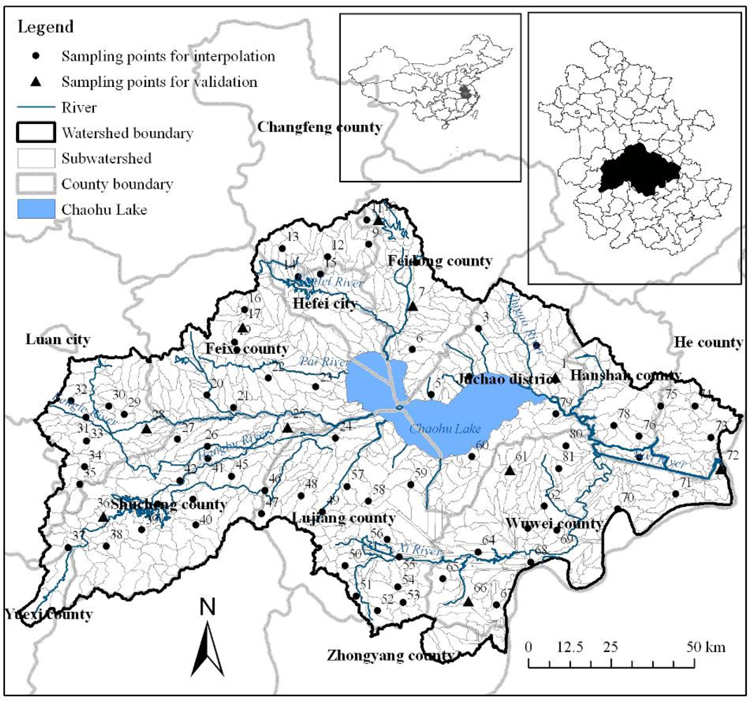
2.1. Study Area
2.2. Surface Soil Survey
2.2.1. Sampling Sites
2.2.2. Laboratory Analysis
2.3. Spatial Interpolation and Validation
2.4. Analysis Method of Spatial Variation
2.5. Analysis Method of Relation
3. Results and Discussion
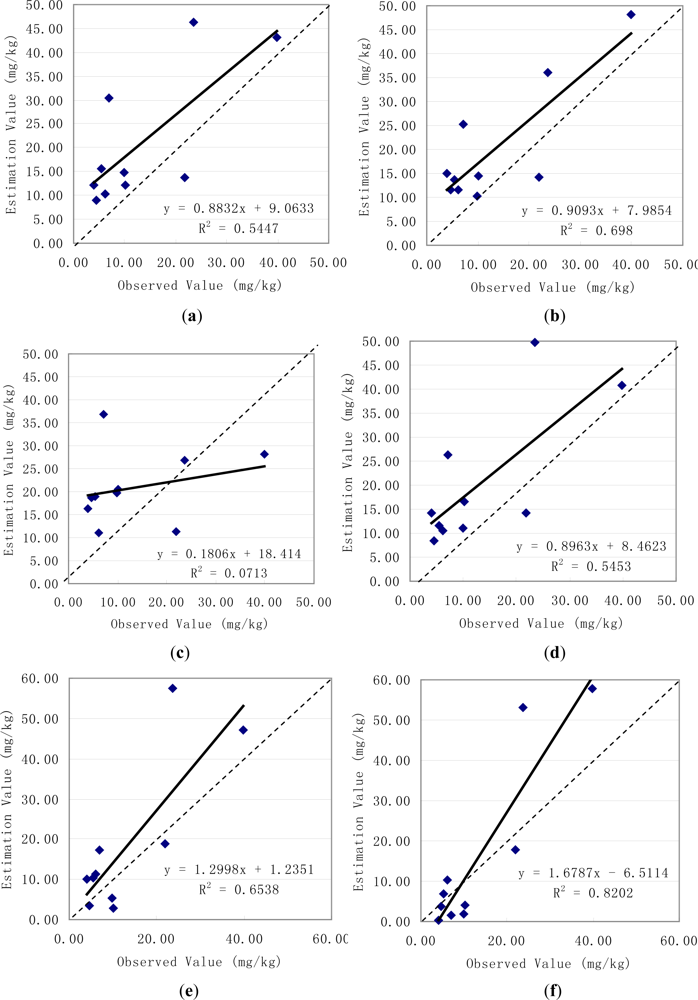
3.1. Validation of Interpolation Results
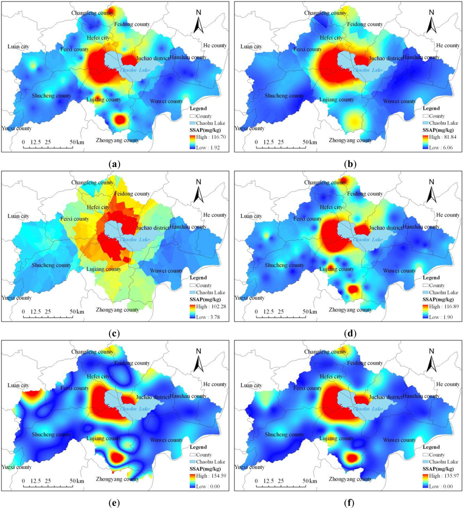
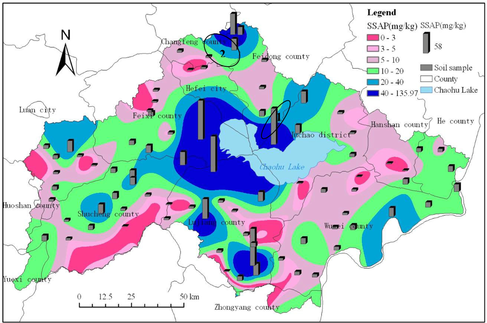
3.2. Spatial Characteristics of Surface Soil Available Phosphorus
3.3. Soil Available Phosphorus under Different Elevation and Slope
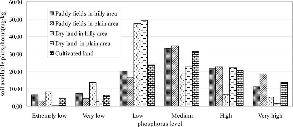
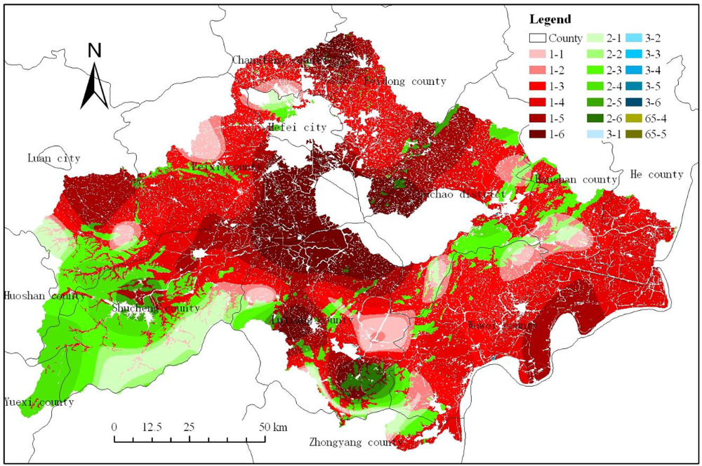
3.4. Soil Available Phosphorus under Different Land Use
3.5. Relation between Subwatershed Scale Soil Available Phosphorus and Environmental Factors
4. Conclusions
- In the prediction of soil available phosphorus in the Chaohu Lake watershed, the Spline Tension method performed the best and then followed by the Spline Regularized method in second, Kriging Ordinary Gaussian method in third and Kriging Ordinary Spherical method the worst.
- The spatial variation of surface soil available phosphorus was high in the Chaohu Lake watershed. The upstream regions around Chaohu Lake, including the west of Chaohu Lake (e.g., southwest of Feixi county, east of Shucheng county and north of Lujiang county) and to the north of Chaohu Lake (e.g., south of Hefei city, south of Feidong county, southwest of Juchao district), had the highest soil available phosphorus content.
- The mean and standard deviation of soil available phosphorus content gradually decreased as the elevation or slope increased. The regions ranging from 0 to 50 meters of elevation were mainly dominated by paddy fields and had the highest soil available phosphorus contents, the regions ranging from 100 to 1480 meters of elevation were mainly dominated by forest land and had the lowest soil available phosphorus contents. The region ranging from 0 to 3 degrees of slope was dominated by cultivated land and had the highest soil available phosphorus content, the regions ranging from 5 to 49.75 degrees of slope were dominated by forest land and had the lowest soil available phosphorus contents. The cultivated land comprised 60.11% of the watershed and of that land 65.63% belonged to the medium to very high SAP level classes, and it played a major role in SAP availability within the watershed and a potential source of phosphorus to Chaohu Lake, resulting in eutrophication. Among the land use types, paddy fields have some of the highest maximum values and variation of coefficients.
- The subwatershed scale soil available phosphorus content and the various environmental factors, including average elevation, slope, precipitation, percentage of cultivated land and percentage of forest land, were significantly correlated, the percentage of construction land, NDVI and soil available phosphorus did not have significant linear relationship. The results after ANOVA and LSD analyses between subwatershed scale soil available phosphorous and five significant environmental factors showed that all the differences were significant (P < 0.05), and E, S, P, PCL1 and PFL had significant effects on subwatershed scale soil available phosphorus. Subwatershed scale soil available phosphorus was decided not only by these environmental factors but also by some other factors such as artificial phosphorus fertilizer application.
Acknowledgments
- Conflict of InterestThe authors declare no conflict of interest.
References
- Li, M; Wu, YJ; Yu, ZL; Sheng, GP; Yu, HQ. Enhanced nitrogen phosphorus removal from eutrophic lake water by Ipomoea aquatica with low-energy ion implantation. Water Res 2009, 43, 1247–1256. [Google Scholar]
- Smith, VH; Tilman, GD; Nekola, JC. Eutrophication: Impacts of excess nutrient inputs on freshwater, marine, and terrestrial ecosystem. Environ. Pollut 1999, 100, 179–196. [Google Scholar]
- Sherwood, LJ; Qualls, RG. Stability of phosphorus within a wetland soil following ferric chloride treatment to control eutrophication. Environ. Sci. Technol 2001, 35, 4126–4131. [Google Scholar]
- Xu, XF; Zhang, CS; Chang, HQ; Wang, FY. A review of water quality and pollution control in China. Amer.-Eur. J. Agric. Environ. Sci 2010, 8, 741–751. [Google Scholar]
- Zare-Mehrjardi, M; Taghizadeh-Mehrjardi, R; Akbarzadeh, A. Evaluation of geostatistical techniques for mapping spatial distribution of soil pH, salinity and plant cover affected by environmental factors in Southern Iran. Not. Sci. Biol 2010, 2, 92–103. [Google Scholar]
- Hosseini, E; Gallichand, D; Marcotte, D. Theoretical and experimental performance of spatial interpolation methods for soil salinity analysis. T. ASAE 1994, 37, 1799–1807. [Google Scholar]
- Sokoti, S; Mahdian, M; Mahmoodi, Sh; Ghahramani, A. Comparing the applicability of some geostatistics methods to predict soil salinity, a case study of Urmia plain. Pajuhesh and Sazandegi 2006, 74, 90–98. (In Persian) [Google Scholar]
- Meul, M; van Meirvenne, M. Kriging soil texture under different types of nonstationarity. Geoderma 2003, 112, 217–233. [Google Scholar]
- Robinson, TP; Metternicht, G. Testing the performance of spatial interpolation techniques for mapping soil properties. Comput. Electron. Agr 2006, 50, 97–108. [Google Scholar]
- Yamashita, N; Ohta, S; Sase, H; Luangjame, J; Visaratana, T; Kievuttinon, B; Garivait, H; Kanzaki, M. Seasonal and spatial variation of nitrogen dynamics in the litter and surface soil layers on a tropical dry evergreen forest slope. Forest Ecol. Manag 2010, 259, 1502–1512. [Google Scholar]
- Zhang, ZM; Yu, XX; Q, S; Li, JW. Spatial variability of soil nitrogen and phosphorus of a mixed forest ecosystem in Beijing, China. Environ. Earth Sci 2010, 60, 1783–1792. [Google Scholar]
- Vaughan, RE; Needelman, RA; Kleinman, PJA; Allen, AL. Spatial variation of soil phosphorus within a drainage Ditch Network. J. Environ. Qual 2007, 36, 1096–1104. [Google Scholar]
- Corazza, EJ; Brossard, M; Muraoka, T; Filho, MAC. Spatial variability of soil phosphorus of a low productivity Brachiaria brizantha pasture. Scientia Agricola 2003, 60, 559–564. [Google Scholar]
- Lin, JS; Shi, XZ; Lu, XX; Yu, DS; Wang, HJ; Zhao, YC; Sun, WX. Storage and spatial variation of phosphorus in paddy soils of China. Pedosphere 2007, 19, 790–798. [Google Scholar]
- Grunwald, S; Reddy, KR; Newman, S; DeBusk, WF. Spatial variability, distribution and uncertainty assessment of soil phosphorus in a south Florida wetland. Environmetrics 2004, 15, 811–825. [Google Scholar]
- Page, T; Haygarth, PM; Beven, KJ; Joynes, A; Butler, T; Keeler, C; Freer, J; Wwens, PN; Wood, GA. Spatial variability of soil phosphorus in relation to the topographic index and critical source areas: sampling for assessing risk to water quality. J. Environ. Qual 2005, 34, 2263–2277. [Google Scholar]
- Zhou, HP; Gao, C; Sun, B; Zhao, HC; Zhang, TL. Spatial variation characteristics and its driving factors of total phosphorus in topsoil of Chaohu Lake watershed. J. AgroEnviron. Sci 2007, 26, 2112–2117. [Google Scholar]
- Zhou, HP; Gao, C. Identifying critical source areas for non-point phosphorus loss in Chaohu watershed. Environ. Sci 2008, 29, 2696–2702. [Google Scholar]
- Olsen, SR; Sommers, LE. Phosphorus. In Methods of Soil Analysis: Chemical and Microbiological Properties; Page, AL, Ed.; ASA and SSSA: Madison, WI, USA, 1982; pp. 403–430. [Google Scholar]
- Environmental Systems Research Institute, Inc (ESRI), ArcGIS Desktop Help 9.2; ESRI: Redlands, CA, USA, 2007; Available online: http://webhelp.esri.com/arcgisdesktop/9.2/index.cfm?TopicName=welcome (accessed on 20 July 2011).
- Willmott, CJ. Some comments on the evaluation of model performance. Bull. Am. Meteorol. Soc 1982, 63, 1309–1313. [Google Scholar]
- Timmermans, WJ; Kustas, WP; Anderson, MC; French, AN. An intercomparison of the surface energy balance algorithm for land SEBAL and the two-source energy balance TSEB modeling schemes. Rem. Sens. Environ 2007, 108, 369–384. [Google Scholar]
- National Soil Survey Office of China, Chinese Soil; China Agricultural Press: Beijing, China, 1998; pp. 1–1252.


| Statistical variable | Description | Equation |
|---|---|---|
| <O> | Mean of the observed variable | |
| <P> | Mean of the model-predicted variable | |
| MD | Mean difference | |
| MAD | Mean absolute difference | |
| MAPD | Mean absolute percent difference |
| Method | Kriging Ordinary Exponential | Kriging Ordinary Gaussian | Kriging Ordinary Spherical | IDW | Spline Regularized | Spline Tension |
|---|---|---|---|---|---|---|
| Pearson correlation coefficient | 0.738* | 0.835** | 0.267 | 0.738* | 0.809** | 0.906** |
| Significance (Two-tailed) | 0.015 | 0.003 | 0.456 | 0.015 | 0.005 | 0.000 |
| Method | <O>(mg/kg) | <P>(mg/kg) | MD(mg/kg) | MAD(mg/kg) | MAPD(%) |
|---|---|---|---|---|---|
| Kriging Ordinary Exponential | 13.25 | 20.77 | 7.52 | 9.12 | 68.78 |
| Kriging Ordinary Gaussian | 13.25 | 20.04 | 6.78 | 8.32 | 62.80 |
| Kriging Ordinary Spherical | 13.25 | 20.81 | 7.55 | 12.05 | 90.92 |
| IDW | 13.25 | 20.34 | 7.09 | 8.62 | 65.04 |
| Spline Regularized | 13.25 | 18.46 | 5.21 | 8.32 | 62.77 |
| Spline Tension | 13.25 | 15.74 | 2.48 | 8.16 | 61.56 |
| Item | Mean (mg/kg) | Minimum (mg/kg) | Maximum (mg/kg) | Range (mg/kg) | Std. Deviation(mg/kg) | Variation coefficient(%) |
|---|---|---|---|---|---|---|
| Soil samples | 18.14 | 1.90 | 116.88 | 114.98 | 24.20 | 133.41 |
| Watershed scale | 22.55 | 0.00 | 135.97 | 135.97 | 26.98 | 119.65 |
| Level code | Level range(mg/kg)* | Level description | Area percentage(%) | Mean (mg/kg) | Std. Deviation(mg/kg) | Variation coefficient(%) |
|---|---|---|---|---|---|---|
| 1 | <3 | Extremely low | 6.72 | 1.71 | 0.87 | 50.88 |
| 2 | 3–5 | Very low | 7.46 | 4.01 | 0.59 | 14.71 |
| 3 | 5–10 | Low | 23.88 | 7.49 | 1.45 | 19.36 |
| 4 | 10–20 | Medium | 30.60 | 14.22 | 2.84 | 19.97 |
| 5 | 20–40 | High | 17.16 | 27.15 | 5.50 | 20.26 |
| 6 | >40 | Very high | 14.18 | 79.96 | 28.75 | 35.96 |
| Elevation level code | Elevation range (m) | Area percentage (%) | Minimum (mg/kg) | Maximum (mg/kg) | Mean (mg/kg) | Std. Deviation (mg/kg) | Variation coefficient (%) |
|---|---|---|---|---|---|---|---|
| 1 | 0–10 | 28.57 | 0.00 | 135.97 | 32.64 | 36.92 | 113.11 |
| 2 | 10–50 | 43.61 | 0.00 | 135.97 | 21.76 | 22.99 | 105.65 |
| 3 | 50–100 | 13.53 | 0.00 | 118.88 | 17.32 | 15.25 | 88.05 |
| 4 | 100–500 | 12.03 | 0.00 | 112.33 | 9.57 | 12.35 | 129.05 |
| 5 | 500–1480 | 2.26 | 0.00 | 18.16 | 9.92 | 5.70 | 57.46 |
| Slope level code | Slope range (degree) | Area percentage (%) | Minimum (mg/kg) | Maximum (mg/kg) | Mean (mg/kg) | Std. Deviation (mg/kg) | Variation coefficient (%) |
|---|---|---|---|---|---|---|---|
| 1 | 0–3 | 78.47 | 0.00 | 135.97 | 25.46 | 28.77 | 113.00 |
| 2 | 3–5 | 4.77 | 0.00 | 135.52 | 15.23 | 17.52 | 115.09 |
| 3 | 5–8 | 3.76 | 0.00 | 133.17 | 13.17 | 15.85 | 120.35 |
| 4 | 8–15 | 6.25 | 0.00 | 119.53 | 11.58 | 14.94 | 128.93 |
| 5 | 15–25 | 5.21 | 0.00 | 119.43 | 9.53 | 12.15 | 127.45 |
| 6 | 25–49.75 | 1.54 | 0.00 | 106.53 | 8.41 | 7.06 | 83.94 |
| Land use type code* | Area percentage (%) | Minimum (mg/kg) | Maximum (mg/kg) | Range (mg/kg) | Mean (mg/kg) | Std. Deviation (mg/kg) | Variation coefficient (%) |
|---|---|---|---|---|---|---|---|
| 112 | 16.14 | 0.00 | 130.75 | 130.75 | 21.97 | 25.27 | 115.02 |
| 113 | 32.39 | 0.00 | 135.97 | 135.97 | 21.97 | 28.03 | 127.58 |
| 122 | 7.14 | 0.00 | 100.22 | 100.22 | 11.75 | 12.88 | 109.62 |
| 123 | 4.44 | 1.32 | 96.27 | 94.95 | 13.94 | 10.35 | 74.25 |
| 21 | 19.60 | 0.00 | 130.67 | 130.67 | 10.63 | 12.95 | 121.83 |
| 22 | 2.06 | 0.00 | 108.13 | 108.13 | 15.75 | 11.99 | 76.13 |
| 23 | 0.03 | 22.71 | 85.02 | 62.32 | 46.84 | 27.37 | 58.43 |
| 24 | 0.03 | 5.28 | 57.54 | 52.26 | 31.59 | 14.59 | 46.19 |
| 31 | 0.03 | 0.03 | 104.81 | 104.78 | 17.45 | 17.06 | 97.77 |
| 32 | 0.01 | 10.43 | 32.07 | 21.65 | 18.44 | 9.08 | 49.24 |
| 65 | 0.001 | 19.95 | 23.18 | 3.23 | 21.51 | 1.23 | 5.72 |
| SAP | E | S | P | PCL1 | PFL | PCL2 | NDVI | |
|---|---|---|---|---|---|---|---|---|
| SAP | 1 | −0.180** | −0.216** | −0.192** | 0.213** | −0.256** | 0.008 | −0.021 |
| E | −0.180** | 1 | 0.898** | 0.345** | −0.640** | 0.747** | −0.177** | 0.568** |
| S | −0.216** | 0.898** | 1 | 0.393** | −0.748** | 0.872** | −0.202** | 0.630** |
| P | −0.192** | 0.345** | 0.393** | 1 | −0.195** | 0.386** | −0.430** | 0.401** |
| PCL1 | 0.213** | −0.640** | −0.748** | −0.195** | 1 | −0.863** | −0.108** | −0.252** |
| PFL | −0.256** | 0.747** | 0.872** | 0.386** | −0.863** | 1 | −0.248** | 0.580** |
| PCL2 | 0.008 | −0.177** | −0.202** | −0.430** | −0.108** | −0.248** | 1 | −0.463** |
| NDVI | −0.021 | 0.568** | 0.630** | 0.401** | −0.252** | 0.580** | −0.463** | 1 |
| level | E | S | P | PCL1 | PFL |
|---|---|---|---|---|---|
| 1 | 29.64a | 24.63a | 23.76a | 11.38a | 27.11a |
| 2 | 22.48b | 15.38b | 33.49b | 15.64ab | 20.00b |
| 3 | 16.46c | 12.41b | 19.07ac | 13.22a | 14.38bc |
| 4 | 9.63d | 9.70b | 15.31c | 22.72bc | 11.11c |
| 5 | 10.86bcde | 8.26b | 10.70c | 26.27c | 11.16c |
| F value | 12.049* | 10.749* | 18.253* | 12.098* | 18.033* |
| Sig. | 0.000 | 0.000 | 0.000 | 0.000 | 0.000 |
© 2011 by the authors; licensee MDPI, Basel, Switzerland. This article is an open-access article distributed under the terms and conditions of the Creative Commons Attribution license (http://creativecommons.org/licenses/by/3.0/).
Share and Cite
Gao, Y.; Gao, J.; Chen, J. Spatial Variation of Surface Soil Available Phosphorous and Its Relation with Environmental Factors in the Chaohu Lake Watershed. Int. J. Environ. Res. Public Health 2011, 8, 3299-3317. https://doi.org/10.3390/ijerph8083299
Gao Y, Gao J, Chen J. Spatial Variation of Surface Soil Available Phosphorous and Its Relation with Environmental Factors in the Chaohu Lake Watershed. International Journal of Environmental Research and Public Health. 2011; 8(8):3299-3317. https://doi.org/10.3390/ijerph8083299
Chicago/Turabian StyleGao, Yongnian, Junfeng Gao, and Jiongfeng Chen. 2011. "Spatial Variation of Surface Soil Available Phosphorous and Its Relation with Environmental Factors in the Chaohu Lake Watershed" International Journal of Environmental Research and Public Health 8, no. 8: 3299-3317. https://doi.org/10.3390/ijerph8083299
APA StyleGao, Y., Gao, J., & Chen, J. (2011). Spatial Variation of Surface Soil Available Phosphorous and Its Relation with Environmental Factors in the Chaohu Lake Watershed. International Journal of Environmental Research and Public Health, 8(8), 3299-3317. https://doi.org/10.3390/ijerph8083299