Abstract
Health disparities are differences in health status across different socioeconomic groups. Classical methods, e.g., the Delta method, have been used to estimate the standard errors of estimated measures of health disparities and to construct confidence intervals for these measures. However, the confidence intervals constructed using the classical methods do not have good coverage properties for situations involving sparse data. In this article, we introduce three new methods to construct fiducial intervals for measures of health disparities based on approximate fiducial quantities. Through a comprehensive simulation study, We compare the empirical coverage properties of the proposed fiducial intervals against two Monte Carlo simulation-based methods—utilizing either a truncated Normal distribution or the Gamma distribution—as well as the classical method. The findings of the simulation study advocate for the adoption of the Monte Carlo simulation-based method with the Gamma distribution when a unified approach is sought for all health disparity measures.
1. Introduction
In recent years, more and more attention has been given to health equity, one of the goals of the Healthy People 2020 [1]. The World Health Organization (WHO) has pointed out the “gap” in health between segments of the population [2]. A health disparity is defined as “a particular type of health difference that is closely linked with social, economic, and/or environmental disadvantage” [1]. The US National Institute on Minority Health and Health Disparities has raised national awareness about the prevalence and impact of health disparities that would adversely affect groups of people who are more vulnerable to health-related issues. Last but not least, the US Centers for Disease Control and Prevention (CDC) has played an important role in identifying the factors that lead to health disparities among racial, ethnic, geographic, and other socioeconomic groups, an example being the 2011 CDC Health Disparities and Inequalities Report [3].
There are multiple measures available to quantify the presence of health disparities across socioeconomic groups. The Health Disparity Calculator (HD*Calc), version 2.0.0, is a free statistical software that calculates estimates of commonly used measures of health disparities and constructs corresponding confidence intervals (CIs), using both classical and Monte Carlo simulation (MCS)-based methods [4,5,6]. The measures implemented in HD*Calc belong to three categories: absolute measures, relative measures and pairwise comparison measures. The absolute measures include range difference (RD), between-group variance (BGV), extended absolute concentration index (eACI) and the slope index of inequality (SII). The relative measures include range ratio (RR), index of disparity (IDisp), mean log deviation (MLD), Theil’s index (T), extended relative concentration index (eRCI), relative index of inequality (RII) and the Kunst–Mackenbach relative index (KMI). The pair comparison methods include pair difference (PD) and pair ratio (PR). Although HD*Calc was designed to analyze data from the Surveillance, Epidemiology, and End Results (SEER) Program, the software can also be used for other population-based health data.
Two articles have formally evaluated the empirical coverage properties of the methods to construct CIs implemented in HD*Calc. The first article has compared the classical method and the MCS-based method using the truncated Normal distribution [7]. The authors concluded that the two methods work well except for situations when the data are sparse. As a general solution to dealing with sparse data, the second article has proposed the use of the MCS-based method with the Gamma distribution [8]. The MCS-based method with the Gamma distribution is currently the recommended approach to construct CIs for the measures of health disparities implemented in HD*Calc. By extending the work from Krishnamoorthy and Lee 2010 [9] to the case of measures of health disparities, the aims of the current article are to introduce three new methods to construct fiducial intervals for measures of health disparities, based on approximate fiducial quantities, and to compare their frequentist properties, i.e., their empirical coverage performance, with those of existing methods by using a simulation study involving nine different scenarios that allow different combinations of sample sizes and true rates per cell (where the cells are all cross-classifications of age groups and socioeconomic groups).
This paper is organized as follows. We review the measures of health disparities implemented in HD*Calc and describe the statistical methods used to construct confidence intervals and fiducial intervals, including the classical method, the MCS-based methods and the proposed new fiducial methods. We describe the simulation study used to evaluate the empirical coverage performance of the intervals constructed using these methods, and, at the end, report and discuss the results of the simulation study. We provide all the results of the simulation study in Appendix A.
2. Materials and Methods
2.1. Background and Notation
In what follows, in contrast to previous work [6,10], we clearly distinguish between functions of parameters and their estimates. We denote by the true rate (e.g., cancer rate) of the k-th age group within the j-th socioeconomic group, . The true age-adjusted rate of the j-th socioeconomic group, , is defined as
where is the weight for the k-th age group within the j-th socioeconomic group.
To estimate the true rate and the true age-adjusted rate , we use the unbiased estimators and , respectively. We denote the estimated rate of the k-th age group within the j-th socioeconomic group as
where denotes the number of events and denotes the number of persons (or person-years). The estimated age-adjusted rate is
We assume that . The variance of the estimator is
An unbiased estimate of this variance is
We define the vector of J estimators/estimates as and the vector of the J true age-adjusted rates as , where for . In what follows, we assume that the J estimators are independent and the estimated variances of these estimators are given by for .
2.2. Measures of Health Disparities
The (true) measures of health disparities are functions of parameters, , although they are often not clearly distinguished from their estimates, which may lead to confusion. Depending on the function , we obtain different measures of health disparities. In what follows, we will present the measures implemented in HD*Calc. For simplicity, we will refer to the (true) age-adjusted rates simply as (true) rates.
2.2.1. Range Difference (RD) and Pair Difference (PD)
The range difference is the difference between the true rates of the best and the worst socioeconomic groups
where and . It is estimated by
where is the j-th order statistic of the observed values of Y. This may cause problems as and may not necessarily be unbiased estimators of and , respectively. To address this issue, we may fix in advance the groups to be compared and consider instead the pair difference
which has as its estimator
where and are estimators of and , respectively.
2.2.2. Between-Group Variance (BGV)
BGV is calculated using the squares of the differences between the socioeconomic groups’ rates and the population mean rate, with weighting by the corresponding population share
where
is the population share of the j-th socioeconomic group (treated as essentially known, i.e., estimated with negligible sampling error), and
is the population mean rate. The estimator of BGV is given by
where .
2.2.3. Range Ratio (RR) and Pair Ratio (PR)
The RR is similar to the RD, where we replace the subtraction with division. It is defined as
where and are defined in (5). It is estimated by
where and are defined in (6).
Similarly to PD, PR is defined as
and is estimated by
where and are estimators of and , respectively.
2.2.4. Relative Concentration Index (RCI) and Extended Relative Concentration Index (eRCI)
RCI is a measure that can be used only with ordinal socioeconomic groups. It is defined by Kakwani et al., 1997 [11] as
where and are defined in (11) and (10), respectively. Here, is the relative rank of the j-th ordinal socioeconomic group, defined as
Yu et al., 2019 [12] used eRCI as a measure of health disparities. It can be calculated as
where is the aversion parameter, and , , and are the same as in (17). The estimator is
If we obtain RCI. In this article, we use for eRCI.
2.2.5. Absolute Concentration Index (ACI) and Extended Absolute Concentration Index (eACI)
ACI is the absolute version of RCI. It has the following formula
which can be estimated by
where and are defined in (10) and (18), respectively.
Yu et al. 2019 [12] used eACI as a measure of health disparities. It can be calculated as
where is the aversion parameter, and , , and are the same as in (22). The estimator is
If we obtain ACI. In this article, we use for eACI.
2.2.6. Slope Index of Inequality (SII)
SII measures the difference in rates between a hypothetical person with and a hypothetical person with . It was introduced by Preston, Haines and Pamuk, 1981 [13] using a simple linear regression model
where is defined in (18) and SII = .
Since the regression is run on grouped data, SII is estimated using the least squares weighted by the population shares
where is defined in (10).
2.2.7. Index of Disparity (IDisp)
The index of disparity (IDisp) measures the relative difference between the rates of the socioeconomic groups and a reference rate as a proportion of the reference rate. It was first introduced by Pearcy and Keppel, 2002 [14] as
A version of IDisp is replacing the population mean rate, , with the rate of a reference group, , which is
The corresponding estimator is
where is the estimator of . To eliminate the absolute values from the formula, HD*Calc recommends the use of the group with the smallest rate as the reference group.
2.2.8. Mean Log Deviation (MLD)
2.2.9. Theil’s Index (T)
2.2.10. Relative Index of Inequality (RII)
2.2.11. Kunst–Mackenbach Relative Index (KMI)
2.3. Confidence Intervals Based on the Classical Method
The classical method used for variance estimation for the majority of the measures of health disparities implemented in HD*Calc is the Delta method. If is an estimator of the true measure of health disparities , we approximate F by using a first-order Taylor series approximation around and then
where is the mean of . Assuming that the J socioeconomic groups are independent, we obtain
where is the main diagonal of the variance-covariance matrix of . We substitute the unknown parameters and with their estimates to obtain , and then construct corresponding Wald confidence intervals for . Detailed derivations of the formulas for the estimated variances may be found in Ahn et al., 2018 [7] for 11 of the 15 measures of health disparities implemented in HD*Calc (all measures except eACI, eRCI, PD and PR) and on the HD*Calc website [4] for all 15 measures.
2.4. Fiducial Intervals
In this section, we describe new methods to construct fiducial intervals for measures of health disparities based on the use of approximate fiducial quantities. The fiducial inference is an approach to inference introduced by Fisher that has good frequentist properties [17,18].
2.4.1. Fiducial Quantities (FQs)
Following Krishnamoorthy and Lee, 2010 [9], for an observed value of the number of events , we have the equalities
and
where is a random variable following a chi-squared distribution with d degree of freedom. Garwood 1936 [19] proposed a related exact confidence interval for a Poisson mean
Cox 1953 [20] introduced an approximate FQ for , . A related approximate fiducial interval is
Dempster 2008 [21] proposed another approximate FQ for , a 50-50 mixture of and .
An approximate FQ for a function of s may be obtained by replacing the s with their FQs in the function [18]. In our case, each measure of health disparities can be expressed as a function of s, and an approximate FQ for
is obtained as
where is an approximate FQ of .
2.4.2. Simulation-Based Methods to Construct Fiducial Intervals
We use the above approximate FQs to construct three different fiducial intervals (FIs):
- FI1.
- Simulate from ;
- FI2.
- Simulate from either or , each with a 50% probability;
- FI3.
- Simulate from both and .
For each method, we plug in the simulated s into the function to obtain the simulated values of the measures of health disparities . After performing B simulations, a 95% FI is constructed using the 2.5 and 97.5 percentiles of the set of simulated values for the measures of health disparities. For cells where no event is observed, i.e., , we follow Zhang et al. 2014 [22] and use
2.5. Monte Carlo Simulation-Based Methods (MCS)
For the Monte Carlo simulation-based methods, we simulate values for the age-adjusted rates, , instead of values for the cell rates , as performed for the previously described fiducial methods, either from a truncated Normal distribution (MCS-N) or a Gamma distribution (MCS-G). The mean and the variance of the distribution from which we simulate values are the estimated mean and the estimated variance of the estimator of . The use of these two distributions ensures that all simulated values are non-negative. When using the truncated Normal distribution, we simulate from a Normal distribution and discard the negative simulated values, i.e., keep only the non-negative simulated values. The adjustment (49) for zero counts is also applied. After we simulate values for , we use them to calculate the simulated values for the measures of health disparities. After performing B simulations, the 95% CI is constructed using the 2.5 and 97.5 percentiles of the set of simulated values for the measures of health disparities.
2.6. Simulation Study
We simulated data under nine different scenarios to allow different combinations of sample sizes and true rates per cell (where the cells are all cross-classifications of age groups and socioeconomic groups). For each scenario, we simulated data for the 12 cells that correspond to the combinations of three ordered socioeconomic groups and four age groups. Fixed weights, according to the WHO World Standard were applied to each age group. Table 1 describes the characteristics of the nine scenarios, with the means and standard deviations (SDs) being calculated across the 12 cells. The combinations of sample sizes and true rates per cell resulted in five categories for the magnitude of the expected count per cell, i.e., <1, 1–9, 10–99, 100–999, and 1000–9999.

Table 1.
Characteristics of the nine scenarios.
For each scenario, we generated 5000 datasets, and for each dataset, we used 5000 simulations to construct the 95% MCS-based CIs and the 95% FIs. The empirical coverage was defined as the frequency of the true value of the measure of health disparities being covered by the nominal 95% CIs or FIs.
3. Results
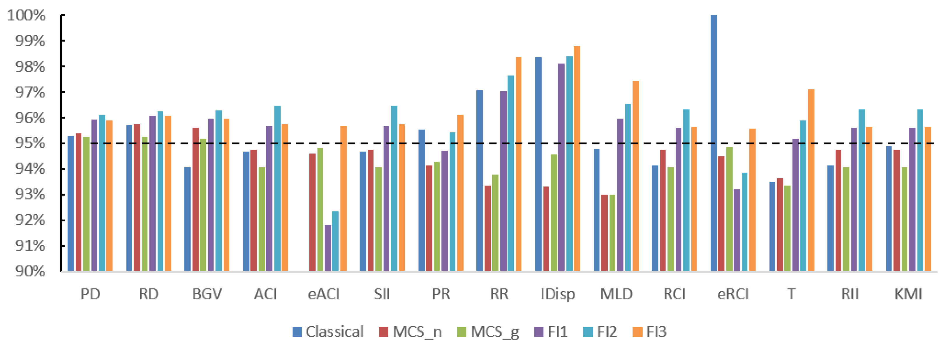
We start with the results for scenario 1, which corresponds to a situation involving extremely sparse data, i.e., where the expected count per cell is below 1. The empirical coverage results are presented in Table 2 and Figure 1. For eACI, the Classic method, FI1 and FI2 had empirical coverages considerably below the nominal 95% level; FI1 and FI2 had the same problem for eRCI. The MCS-N method had only about 91% empirical coverage for PD, while FI3 had very large empirical coverage ranging from 99% to 100% for 11 of the 15 measures. By contrast, the MCS-G method performed reasonably well for all 15 measures for this scenario.
Table 2.
Empirical coverage (%) for nominal 95% confidence intervals and fiducial intervals for scenario 1.
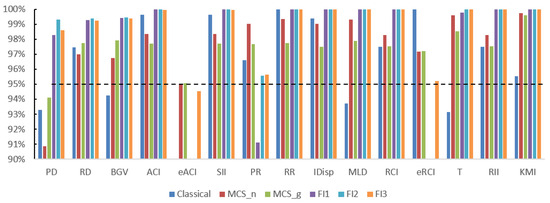
Figure 1.
Empirical coverage results for scenario 1. The dashed line shows 95% coverage.
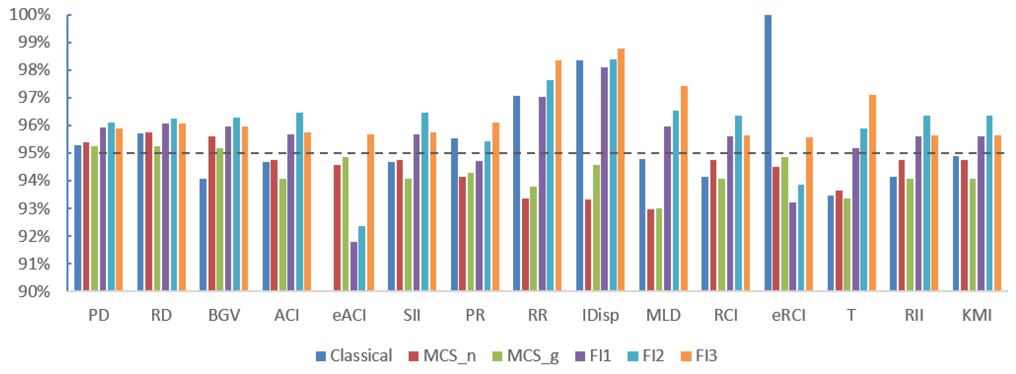
The results for scenarios 2 and 3 were very similar to each other. They both correspond to situations involving sparse (but not extremely sparse) data, where the expected count per cell is between 1 and 10. The empirical coverage results are shown in Table 3 and Figure 2 for scenario 2, and in Table 4 and Figure 3 for scenario 3, respectively. For both scenarios, the Classic method still had empirical coverages considerably below the nominal 95% level for eACI. FI1 and FI2 had the same problem for eACI, but to a much lesser extent, with empirical coverages of about 92%. Overall, FI3 performed best for the 15 measures, followed closely by MCS-G and MCS-N.
Table 3.
Empirical coverage (%) for nominal 95% confidence intervals and fiducial intervals for scenario 2.
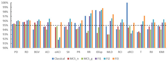
Figure 2.
Empirical coverage results for scenario 2. The dashed line shows 95% coverage.
Table 4.
Empirical coverage (%) for nominal 95% confidence intervals and fiducial intervals for scenario 3.
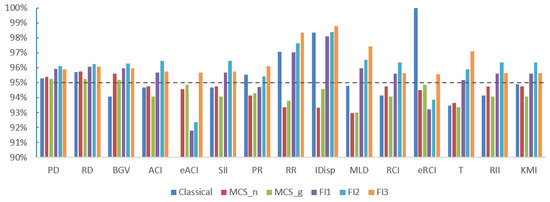
Figure 3.
Empirical coverage results for scenario 3. The dashed line shows 95% coverage.
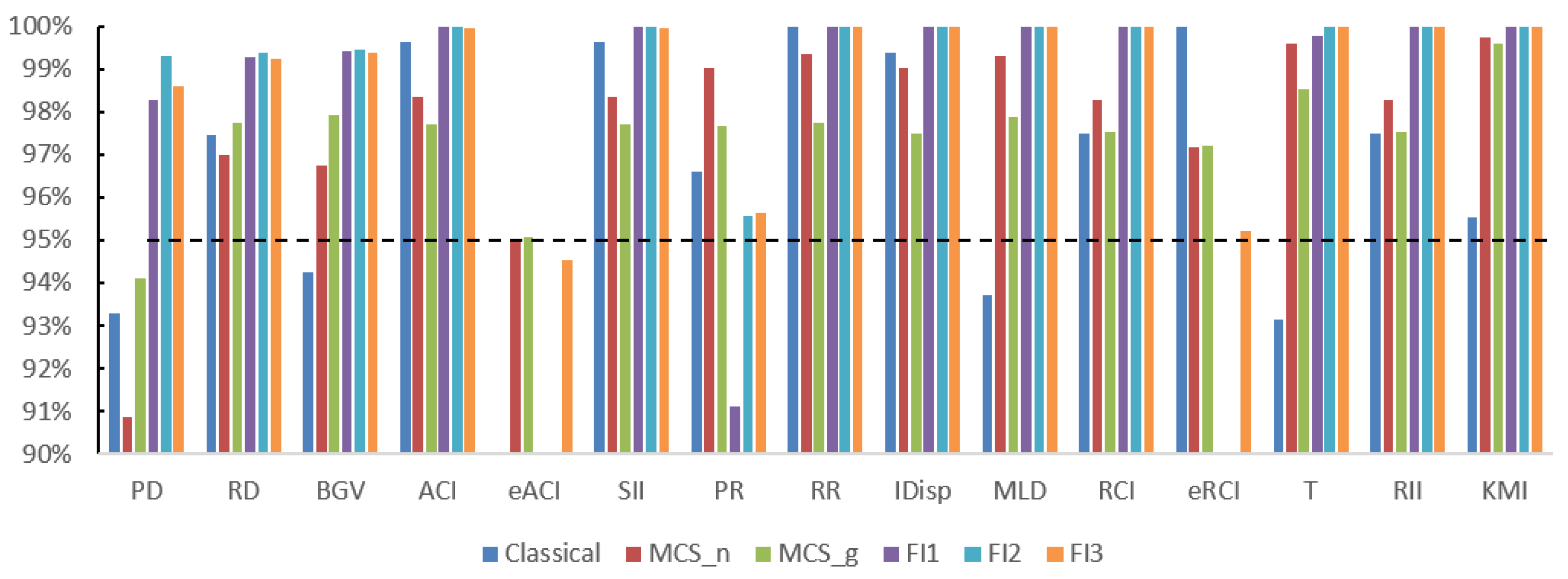
For scenarios 4 to 9, where the data may not be considered sparse by having an expected count per cell of 10 or more, the empirical coverages are between 94% and 96% for all methods and all 15 measures, except for the Classical method for eACI (where they ranged from 79% to 83%) and eRCI (where they were all 100%). For these scenarios, all methods except the Classical method performed well. The complete results regarding the empirical coverage are shown in Appendix A.
4. Discussion
We compared six methods to construct confidence intervals and fiducial intervals for 15 measures of health disparities with regard to their empirical coverage under nine different scenarios. Overall, two methods performed well: the MCS-G method to construct confidence intervals and the FI3 method to construct fiducial intervals. It is important to note that the documentation for HD*Calc version 2.0.0 also recommends the use of the Monte Carlo simulation-based method with the Gamma distribution based on the results from Ahn et al., 2019 [8] regarding 11 measures of health disparities. Compared to the Normal distribution, the Gamma distribution is a better choice to use for simulating rates due to its positivity. Moreover, its flexibility in accommodating asymmetry surpasses that of a truncated Normal distribution.
The strengths of the current study include the addition of four measures (eACI, eRCI, PD and PR) to the list of 11 measures of health disparities previously investigated, and the consideration of different scenarios corresponding to different combinations of sample sizes and true rates per cell. The limitations, due to feasibility reasons, include the consideration of eACI and eRCI only when the aversion parameter , the use of only one value for the number of simulations used for the MCS-based methods and the fiducial methods, i.e., 5000 simulations, the use of an ordinal socioeconomic group variable with only three levels, and the use of an age group variable with only four levels.
Future research work should consider eACI and eRCI with other values of the aversion parameter, a larger number of socioeconomic groups and age groups, and different numbers of simulations for the MCS-based methods and the fiducial methods. Building upon the work from Talih et al., 2020 [23], related future research should also investigate if it is possible to reduce a large number of measures of health disparities to a smaller set of measures that satisfy a set of desirable properties and are easier to interpret. With a smaller number of recommended measures of health disparities, it would be easier to thoroughly compare the performance of statistical methods to construct confidence intervals and fiducial intervals for these selected measures.
5. Conclusions
Given that the MCS-G method is much simpler to understand and implement than the FI3 method, and the lack of familiarity of statisticians and (more importantly) practitioners with fiducial methods and fiducial intervals, we recommend the use of the Monte Carlo simulation-based method with the Gamma distribution.
Author Contributions
Conceptualization, T.L., A.D.D. and G.L.; methodology, T.L. and G.L.; software, T.L.; formal analysis, T.L.; investigation, T.L., A.D.D. and G.L.; writing—original draft preparation, T.L.; writing—review and editing, A.D.D. and G.L.; visualization, T.L. All authors have read and agreed to the published version of the manuscript.
Funding
This research received no external funding.
Institutional Review Board Statement
Not applicable.
Informed Consent Statement
Not applicable.
Data Availability Statement
The code used to simulate the data for this study is available upon request from the corresponding author.
Conflicts of Interest
The authors declare no conflicts of interest.
Abbreviations
The following abbreviations are used in this manuscript:
| ACI | absolute concentration index |
| BGV | between-group variance |
| CDC | Centers for Disease Control and Prevention |
| CI | confidence interval |
| eACI | extended absolute concentration index |
| eRCI | extended relative concentration index |
| FI | fiducial interval |
| FQ | fiducial quantity |
| HD*Calc | Health Disparity Calculator |
| IDisp | index of disparity |
| KMI | Kunst-Mackenbach relative index |
| MCS | Monte Carlo simulation |
| MCS-N | Monte Carlo simulation-based using a truncated Normal distribution |
| MCS-G | Monte Carlo simulation-based using the Gamma distribution |
| MLD | mean log deviation |
| PD | pair difference |
| PR | pair ratio |
| RCI | relative concentration index |
| RD | range difference |
| RII | relative index of inequality |
| RR | range ratio |
| SEER | Surveillance, Epidemiology, and End Results |
| SII | slope index of inequality |
| T | Theil’s index |
| WHO | World Health Organization |
Appendix A. Results of the Simulation Study
Table A1.
Empirical coverage (%) for nominal 95% confidence intervals and fiducial intervals for all scenarios.
Table A1.
Empirical coverage (%) for nominal 95% confidence intervals and fiducial intervals for all scenarios.
| Measure | Scenario | Classical | MCS-N | MCS-G | FI1 | FI2 | FI3 |
|---|---|---|---|---|---|---|---|
| PD | 1 | 93.28 | 90.86 | 94.12 | 98.30 | 99.32 | 98.60 |
| 2 | 95.28 | 95.38 | 95.26 | 95.92 | 96.10 | 95.90 | |
| 3 | 95.28 | 95.38 | 95.26 | 95.92 | 96.10 | 95.90 | |
| 4 | 95.28 | 95.32 | 95.40 | 95.40 | 95.20 | 95.30 | |
| 5 | 95.28 | 95.32 | 95.40 | 95.40 | 95.20 | 95.30 | |
| 6 | 95.28 | 95.32 | 95.40 | 95.40 | 95.20 | 95.30 | |
| 7 | 94.66 | 94.74 | 94.78 | 94.74 | 94.76 | 94.72 | |
| 8 | 94.66 | 94.74 | 94.78 | 94.74 | 94.76 | 94.72 | |
| 9 | 94.80 | 94.78 | 94.80 | 94.78 | 94.78 | 94.92 | |
| RD | 1 | 97.46 | 97.00 | 97.74 | 99.30 | 99.38 | 99.26 |
| 2 | 95.70 | 95.76 | 95.26 | 96.08 | 96.24 | 96.06 | |
| 3 | 95.70 | 95.76 | 95.26 | 96.08 | 96.24 | 96.06 | |
| 4 | 95.28 | 95.36 | 95.40 | 95.40 | 95.18 | 95.28 | |
| 5 | 95.28 | 95.36 | 95.40 | 95.40 | 95.18 | 95.28 | |
| 6 | 95.28 | 95.36 | 95.40 | 95.40 | 95.18 | 95.28 | |
| 7 | 94.66 | 94.74 | 94.78 | 94.74 | 94.76 | 94.72 | |
| 8 | 94.66 | 94.74 | 94.78 | 94.74 | 94.76 | 94.72 | |
| 9 | 94.80 | 94.78 | 94.80 | 94.78 | 94.78 | 94.92 | |
| BGV | 1 | 94.26 | 96.74 | 97.94 | 99.42 | 99.46 | 99.38 |
| 2 | 94.08 | 95.60 | 95.18 | 95.98 | 96.28 | 95.98 | |
| 3 | 94.08 | 95.60 | 95.18 | 95.98 | 96.28 | 95.98 | |
| 4 | 95.06 | 95.06 | 95.12 | 95.10 | 95.12 | 95.08 | |
| 5 | 95.06 | 95.06 | 95.12 | 95.10 | 95.12 | 95.08 | |
| 6 | 95.06 | 95.06 | 95.12 | 95.10 | 95.12 | 95.08 | |
| 7 | 95.24 | 95.40 | 95.18 | 95.36 | 95.30 | 95.34 | |
| 8 | 95.24 | 95.40 | 95.18 | 95.36 | 95.30 | 95.34 | |
| 9 | 94.80 | 94.76 | 94.88 | 94.86 | 94.84 | 94.82 | |
| ACI | 1 | 99.64 | 98.34 | 97.72 | 99.98 | 100.0 | 99.96 |
| 2 | 94.68 | 94.76 | 94.06 | 95.68 | 96.48 | 95.74 | |
| 3 | 94.68 | 94.76 | 94.06 | 95.68 | 96.48 | 95.74 | |
| 4 | 95.40 | 95.48 | 95.12 | 95.40 | 95.56 | 95.40 | |
| 5 | 95.40 | 95.48 | 95.12 | 95.40 | 95.56 | 95.40 | |
| 6 | 95.40 | 95.48 | 95.12 | 95.40 | 95.56 | 95.40 | |
| 7 | 94.54 | 94.48 | 94.54 | 94.68 | 94.42 | 94.54 | |
| 8 | 94.54 | 94.48 | 94.54 | 94.68 | 94.42 | 94.54 | |
| 9 | 94.62 | 94.70 | 94.72 | 94.60 | 94.62 | 94.64 | |
| eACI | 1 | 82.82 | 95.04 | 95.08 | 52.20 | 64.10 | 94.52 |
| 2 | 78.94 | 94.60 | 94.82 | 91.80 | 92.36 | 95.68 | |
| 3 | 78.70 | 94.58 | 94.84 | 91.80 | 92.34 | 95.66 | |
| 4 | 81.46 | 94.42 | 94.60 | 94.10 | 94.20 | 94.40 | |
| 5 | 79.38 | 94.50 | 94.62 | 94.06 | 94.10 | 94.40 | |
| 6 | 79.24 | 94.52 | 94.62 | 94.04 | 94.12 | 94.40 | |
| 7 | 81.78 | 95.28 | 95.20 | 95.24 | 95.36 | 95.26 | |
| 8 | 80.14 | 95.22 | 95.20 | 95.24 | 95.32 | 95.30 | |
| 9 | 83.10 | 95.54 | 95.54 | 95.56 | 95.52 | 95.46 | |
| SII | 1 | 99.64 | 98.34 | 97.72 | 99.98 | 100.0 | 99.96 |
| 2 | 94.68 | 94.76 | 94.06 | 95.68 | 96.48 | 95.74 | |
| 3 | 94.68 | 94.76 | 94.06 | 95.68 | 96.48 | 95.74 | |
| 4 | 95.40 | 95.48 | 95.12 | 95.40 | 95.56 | 95.40 | |
| 5 | 95.40 | 95.48 | 95.12 | 95.40 | 95.56 | 95.40 | |
| 6 | 95.40 | 95.48 | 95.12 | 95.40 | 95.56 | 95.40 | |
| 7 | 94.54 | 94.48 | 94.54 | 94.68 | 94.42 | 94.54 | |
| 8 | 94.54 | 94.48 | 94.54 | 94.68 | 94.42 | 94.54 | |
| 9 | 94.62 | 94.70 | 94.72 | 94.60 | 94.62 | 94.64 | |
| PR | 1 | 96.62 | 99.04 | 97.66 | 91.12 | 95.56 | 95.64 |
| 2 | 95.52 | 94.14 | 94.30 | 94.72 | 95.42 | 96.10 | |
| 3 | 95.52 | 94.14 | 94.30 | 94.72 | 95.42 | 96.10 | |
| 4 | 95.66 | 95.64 | 95.44 | 95.36 | 95.62 | 95.62 | |
| 5 | 95.66 | 95.64 | 95.44 | 95.36 | 95.62 | 95.62 | |
| 6 | 95.66 | 95.64 | 95.44 | 95.36 | 95.62 | 95.62 | |
| 7 | 94.80 | 94.88 | 94.80 | 94.68 | 94.80 | 94.84 | |
| 8 | 94.80 | 94.88 | 94.80 | 94.68 | 94.80 | 94.84 | |
| 9 | 94.94 | 94.84 | 94.82 | 94.92 | 94.98 | 94.98 | |
| RR | 1 | 100.0 | 99.36 | 97.76 | 100.0 | 100.0 | 100.0 |
| 2 | 97.08 | 93.34 | 93.80 | 97.04 | 97.64 | 98.36 | |
| 3 | 97.08 | 93.34 | 93.80 | 97.04 | 97.64 | 98.36 | |
| 4 | 95.68 | 95.70 | 95.54 | 95.44 | 95.70 | 95.68 | |
| 5 | 95.68 | 95.70 | 95.54 | 95.44 | 95.70 | 95.68 | |
| 6 | 95.68 | 95.70 | 95.54 | 95.44 | 95.70 | 95.68 | |
| 7 | 94.80 | 94.88 | 94.80 | 94.68 | 94.80 | 94.84 | |
| 8 | 94.80 | 94.88 | 94.80 | 94.68 | 94.80 | 94.84 | |
| 9 | 94.94 | 94.84 | 94.82 | 94.92 | 94.98 | 94.98 | |
| IDisp | 1 | 99.40 | 99.04 | 97.50 | 100.0 | 100.0 | 100.0 |
| 2 | 98.36 | 93.32 | 94.58 | 98.10 | 98.40 | 98.78 | |
| 3 | 98.36 | 93.32 | 94.58 | 98.10 | 98.40 | 98.78 | |
| 4 | 95.14 | 95.58 | 95.42 | 95.32 | 95.48 | 95.56 | |
| 5 | 95.14 | 95.58 | 95.42 | 95.32 | 95.48 | 95.56 | |
| 6 | 95.14 | 95.58 | 95.42 | 95.32 | 95.48 | 95.56 | |
| 7 | 94.80 | 94.44 | 94.64 | 94.70 | 94.58 | 94.68 | |
| 8 | 94.80 | 94.44 | 94.64 | 94.70 | 94.58 | 94.68 | |
| 9 | 94.92 | 94.88 | 94.82 | 94.86 | 94.88 | 94.96 | |
| MLD | 1 | 93.72 | 99.32 | 97.88 | 99.98 | 100.0 | 100.0 |
| 2 | 94.80 | 92.98 | 93.00 | 95.98 | 96.54 | 97.44 | |
| 3 | 94.80 | 92.98 | 93.00 | 95.98 | 96.54 | 97.44 | |
| 4 | 95.70 | 95.06 | 95.10 | 95.74 | 95.82 | 96.06 | |
| 5 | 95.70 | 95.06 | 95.10 | 95.74 | 95.82 | 96.06 | |
| 6 | 95.70 | 95.06 | 95.10 | 95.74 | 95.82 | 96.06 | |
| 7 | 95.02 | 95.14 | 95.02 | 94.98 | 95.00 | 95.06 | |
| 8 | 95.02 | 95.14 | 95.02 | 94.98 | 95.00 | 95.06 | |
| 9 | 94.84 | 94.78 | 94.92 | 94.70 | 94.84 | 94.80 | |
| RCI | 1 | 97.50 | 98.30 | 97.54 | 99.98 | 100.0 | 100.0 |
| 2 | 94.14 | 94.76 | 94.06 | 95.62 | 96.34 | 95.64 | |
| 3 | 94.14 | 94.76 | 94.06 | 95.62 | 96.34 | 95.64 | |
| 4 | 95.28 | 95.46 | 95.04 | 95.22 | 95.56 | 95.34 | |
| 5 | 95.28 | 95.46 | 95.04 | 95.22 | 95.56 | 95.34 | |
| 6 | 95.28 | 95.46 | 95.04 | 95.22 | 95.56 | 95.34 | |
| 7 | 94.60 | 94.62 | 94.64 | 94.62 | 94.64 | 94.70 | |
| 8 | 94.60 | 94.62 | 94.64 | 94.62 | 94.64 | 94.70 | |
| 9 | 94.90 | 94.86 | 94.88 | 94.78 | 94.84 | 94.82 | |
| eRCI | 1 | 100.0 | 97.16 | 97.22 | 71.58 | 80.94 | 95.20 |
| 2 | 100.0 | 94.50 | 94.84 | 93.22 | 93.86 | 95.58 | |
| 3 | 100.0 | 94.50 | 94.84 | 93.22 | 93.86 | 95.58 | |
| 4 | 100.0 | 95.02 | 95.14 | 95.08 | 95.10 | 95.46 | |
| 5 | 100.0 | 95.02 | 95.14 | 95.08 | 95.10 | 95.46 | |
| 6 | 100.0 | 95.02 | 95.14 | 95.08 | 95.10 | 95.46 | |
| 7 | 100.0 | 94.82 | 94.76 | 94.80 | 94.86 | 94.86 | |
| 8 | 100.0 | 94.82 | 94.76 | 94.80 | 94.86 | 94.86 | |
| 9 | 100.0 | 95.38 | 95.40 | 95.38 | 95.12 | 95.28 | |
| T | 1 | 93.14 | 99.60 | 98.54 | 99.78 | 99.98 | 99.98 |
| 2 | 93.48 | 93.64 | 93.36 | 95.16 | 95.90 | 97.10 | |
| 3 | 93.48 | 93.64 | 93.36 | 95.16 | 95.90 | 97.10 | |
| 4 | 95.52 | 95.12 | 95.20 | 95.64 | 95.70 | 95.92 | |
| 5 | 95.52 | 95.12 | 95.20 | 95.64 | 95.70 | 95.92 | |
| 6 | 95.52 | 95.12 | 95.20 | 95.64 | 95.70 | 95.92 | |
| 7 | 95.20 | 95.06 | 95.06 | 95.16 | 95.16 | 95.16 | |
| 8 | 95.20 | 95.06 | 95.06 | 95.16 | 95.16 | 95.16 | |
| 9 | 94.88 | 94.82 | 94.92 | 94.78 | 94.76 | 94.84 | |
| RII | 1 | 97.50 | 98.30 | 97.54 | 99.98 | 100.0 | 100.0 |
| 2 | 94.14 | 94.76 | 94.06 | 95.62 | 96.34 | 95.64 | |
| 3 | 94.14 | 94.76 | 94.06 | 95.62 | 96.34 | 95.64 | |
| 4 | 95.28 | 95.46 | 95.04 | 95.22 | 95.56 | 95.34 | |
| 5 | 95.28 | 95.46 | 95.04 | 95.22 | 95.56 | 95.34 | |
| 6 | 95.28 | 95.46 | 95.04 | 95.22 | 95.56 | 95.34 | |
| 7 | 94.60 | 94.62 | 94.64 | 94.62 | 94.64 | 94.70 | |
| 8 | 94.60 | 94.62 | 94.64 | 94.62 | 94.64 | 94.70 | |
| 9 | 94.90 | 94.86 | 94.88 | 94.78 | 94.84 | 94.82 | |
| KMI | 1 | 95.54 | 99.76 | 99.62 | 99.98 | 100.0 | 100.0 |
| 2 | 94.90 | 94.76 | 94.06 | 95.62 | 96.34 | 95.64 | |
| 3 | 94.90 | 94.76 | 94.06 | 95.62 | 96.34 | 95.64 | |
| 4 | 95.18 | 95.46 | 95.04 | 95.22 | 95.56 | 95.34 | |
| 5 | 95.18 | 95.46 | 95.04 | 95.22 | 95.56 | 95.34 | |
| 6 | 95.18 | 95.46 | 95.04 | 95.22 | 95.56 | 95.34 | |
| 7 | 94.66 | 94.62 | 94.64 | 94.62 | 94.64 | 94.70 | |
| 8 | 94.66 | 94.62 | 94.64 | 94.62 | 94.64 | 94.70 | |
| 9 | 94.84 | 94.86 | 94.88 | 94.78 | 94.84 | 94.82 |
References
- U.S. Department of Health and Human Services, Office of Disease Prevention and Health Promotion. Healthy People 2020. 2010. Available online: https://www.cdc.gov/nchs/healthy_people/hp2020.htm (accessed on 1 September 2023).
- Marmot, M.; Friel, S.; Bell, R.; Houweling, T.A.; Taylor, S.; on behalf of the Commission on Social Determinants of Health. Closing the gap in a generation: Health equity through action on the social determinants of health. Lancet 2008, 372, 1661–1669. [Google Scholar] [CrossRef] [PubMed]
- Truman, B.I.; Centers for Disease Control and Prevention. CDC health disparities and inequalities report-United States, 2011. Mickey Leland Cent. Inf. Portal 2011, 4. Available online: https://digitalscholarship.tsu.edu/mlcejs_info/4/ (accessed on 1 September 2023).
- Division of Cancer Control and Population Sciences, National Cancer Institute. Health Disparities Calculator (HD*Calc), Version 2.0.0. 2019. Available online: https://seer.cancer.gov/hdcalc/ (accessed on 1 September 2023).
- Breen, N.; Scott, S.; Percy-Laurry, A.; Lewis, D.; Glasgow, R. Health disparities calculator: A methodologically rigorous tool for analyzing inequalities in population health. Am. J. Public Health 2014, 104, 1589–1591. [Google Scholar] [CrossRef]
- Harper, S.; Lynch, J. Methods for Measuring Cancer Disparities: Using Data Relevant to Healthy People 2010 Cancer-Related Objectives; NCI Cancer Surveillance Monograph Series, No. 6; Technical Report; NIH Pub. No. 05-5777; National Cancer Institute: Bethesda, MD, USA, 2005.
- Ahn, J.; Harper, S.; Yu, M.; Feuer, E.J.; Liu, B.; Luta, G. Variance Estimation and Confidence Intervals for 11 Commonly Used Health Disparity Measures. JCO Clin. Cancer Inform. 2018, 2, 2. [Google Scholar] [CrossRef] [PubMed]
- Ahn, J.; Harper, S.; Yu, M.; Feuer, E.J.; Liu, B. Improved Monte Carlo methods for estimating confidence intervals for eleven commonly used health disparity measures. PLoS ONE 2019, 14, e0219542. [Google Scholar] [CrossRef] [PubMed]
- Krishnamoorthy, K.; Lee, M. Inference for functions of parameters in discrete distributions based on fiducial approach: Binomial and Poisson cases. J. Stat. Plan. Inference 2010, 140, 1182–1192. [Google Scholar] [CrossRef]
- Harper, S.; Lynch, J. Selected Comparisons of Measures of Health Disparities: A Review Using Databases Relevant to Healthy People 2010 Cancer-Related Objectives; NCI Cancer Surveillance Monograph Series, No. 7; Technical Report; NIH Pub. No. 07-6281; National Cancer Institute: Bethesda, MD, USA, 2007.
- Kakwani, N.; Wagstaff, A.; Van Doorslaer, E. Socioeconomic inequalities in health: Measurement, computation, and statistical inference. J. Econom. 1997, 77, 87–103. [Google Scholar] [CrossRef]
- Yu, M.; Liu, B.; Li, Y.; Zou, Z.; Breen, N. Statistical inferences of extended concentration indices for directly standardized rates. Stat. Med. 2019, 38, 62–73. [Google Scholar] [CrossRef]
- Preston, S.H.; Haines, M.R.; Pamuk, E. Effects of Industrialization and Urbanization on Mortality in Developed Countries; Department of Economics, Wayne State University: Detroit, MI, USA, 1981. [Google Scholar]
- Pearcy, J.N.; Keppel, K.G. A Summary Measure of Health Disparity. Public Health Rep. 2002, 117, 273–280. [Google Scholar] [CrossRef] [PubMed]
- Pamuk, E.R. Social-class inequality in infant mortality in England and Wales from 1921 to 1980. Eur. J. Popul./Revue Européenne Démographie 1988, 4, 1–21. [Google Scholar] [CrossRef]
- Mackenbach, J.P.; Kunst, A.E. Measuring the magnitude of socio-economic inequalities in health: An overview of available measures illustrated with two examples from Europe. Soc. Sci. Med. 1997, 44, 757–771. [Google Scholar] [CrossRef]
- Fisher, R.A. Inverse probability. Math. Proc. Camb. Philos. Soc. 1930, 26, 528–535. [Google Scholar] [CrossRef]
- Fisher, R.A. The fiducial argument in statistical inference. Ann. Eugen. 1935, 6, 391–398. [Google Scholar] [CrossRef]
- Garwood, F. Fiducial limits for the Poisson distribution. Biometrika 1936, 28, 437–442. [Google Scholar]
- Cox, D. Some simple approximate tests for Poisson variates. Biometrika 1953, 40, 354–360. [Google Scholar] [CrossRef]
- Dempster, A.P. The Dempster–Shafer calculus for statisticians. Int. J. Approx. Reason. 2008, 48, 365–377. [Google Scholar] [CrossRef]
- Zhang, S.; Luo, J.; Zhu, L.; Stinchcomb, D.G.; Campbell, D.; Carter, G.; Gilkeson, S.; Feuer, E.J. Confidence intervals for ranks of age-adjusted rates across states or counties. Stat. Med. 2014, 33, 1853–1866. [Google Scholar] [CrossRef] [PubMed]
- Talih, M.; Moonesinghe, R.; Huang, D.T. Measuring the Magnitude of Health Inequality between 2 Population Subgroup Proportions. Am. J. Epidemiol. 2020, 189, 987–996. [Google Scholar] [CrossRef]
Disclaimer/Publisher’s Note: The statements, opinions and data contained in all publications are solely those of the individual author(s) and contributor(s) and not of MDPI and/or the editor(s). MDPI and/or the editor(s) disclaim responsibility for any injury to people or property resulting from any ideas, methods, instructions or products referred to in the content. |
© 2024 by the authors. Licensee MDPI, Basel, Switzerland. This article is an open access article distributed under the terms and conditions of the Creative Commons Attribution (CC BY) license (https://creativecommons.org/licenses/by/4.0/).