
Automatic Detection of Oral Squamous Cell Carcinoma from Histopathological Images of Oral Mucosa Using Deep Convolutional Neural Network

Abstract
1. Introduction
1.1. Contribution
1.2. Organization
2. Related Work
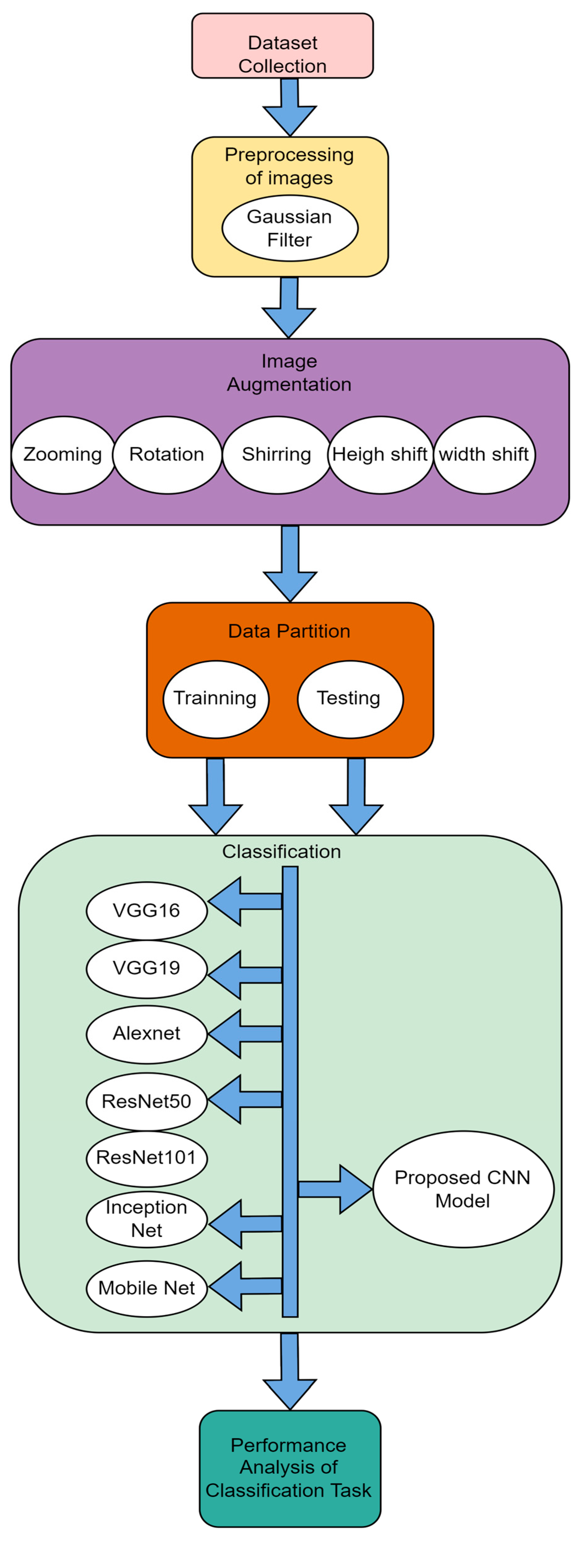
3. Methods and Techniques Used
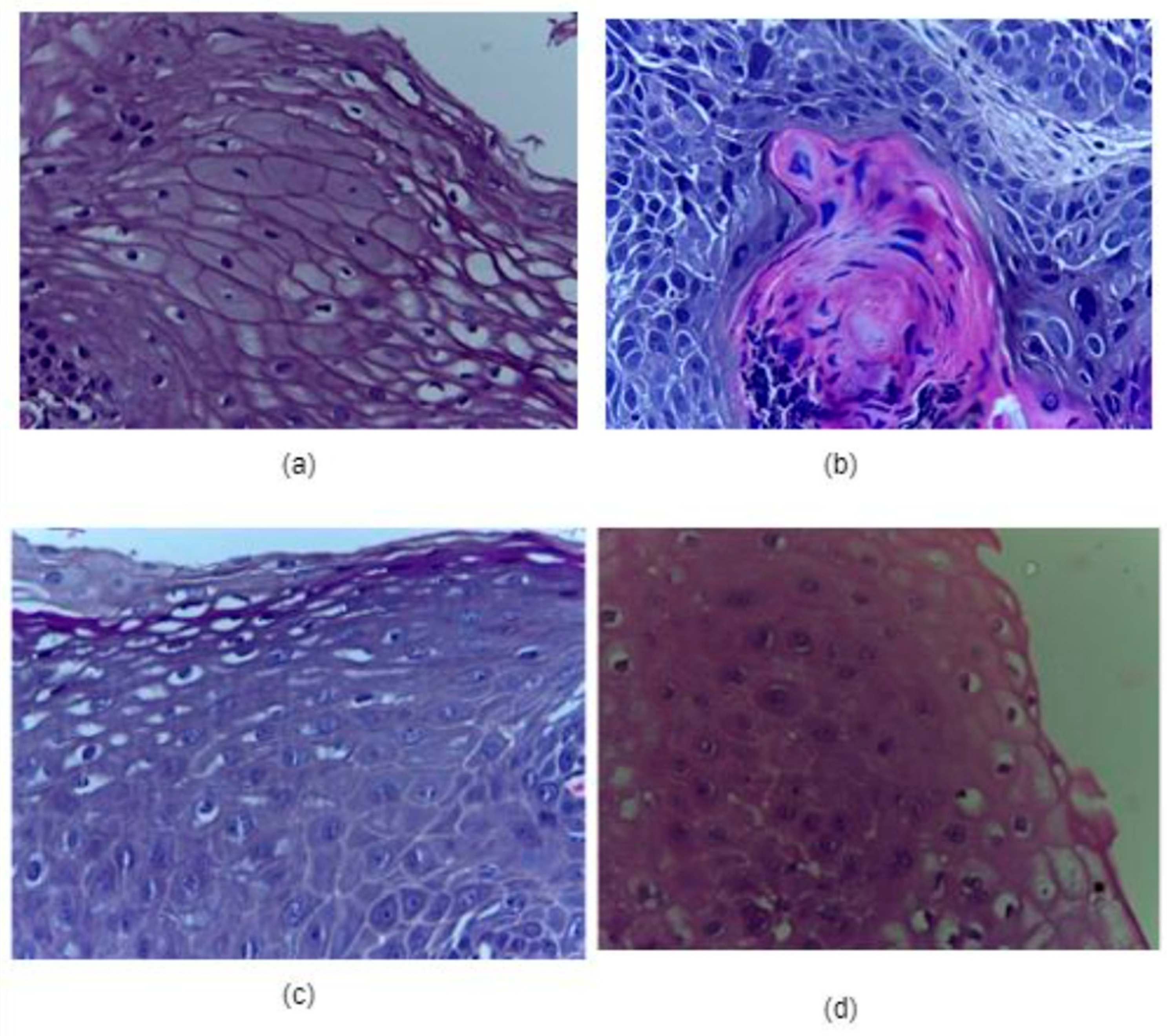
3.1. Dataset Used
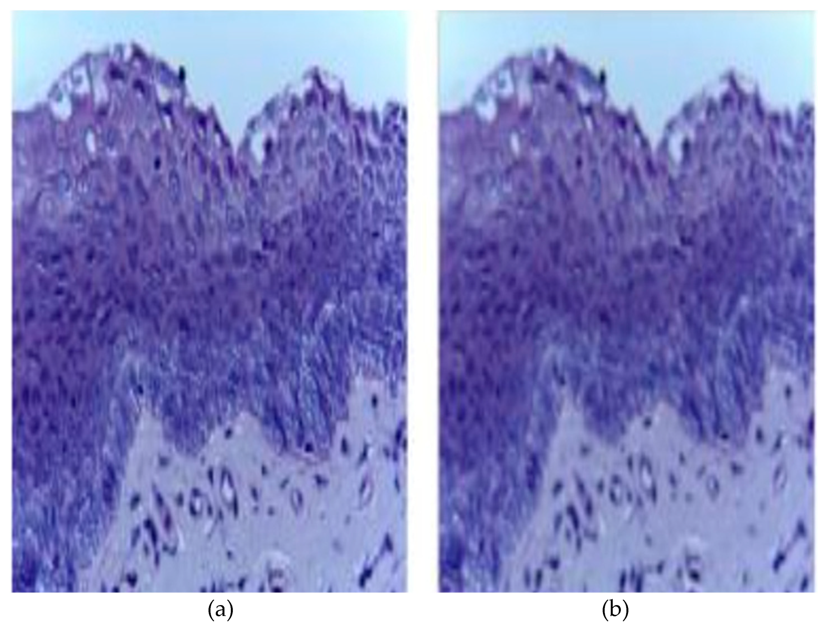
3.2. Image Preprocessing:
3.3. Image Augmentation
3.4. Data Partition
4. Proposed Methodology
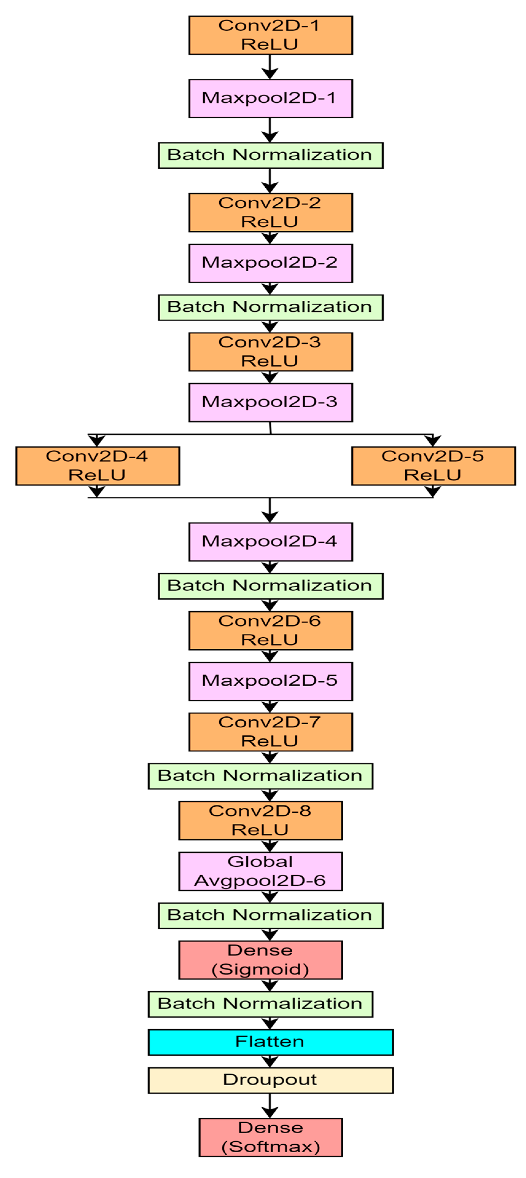
4.1. Proposed 10-Layer CNN Architecture
5. Experimental Studies
Hyper Parameter Setting of the 10-Layer CNN
6. Performance Evaluation and Result Analysis
6.1. Performance Evaluation Using Statistical Measure
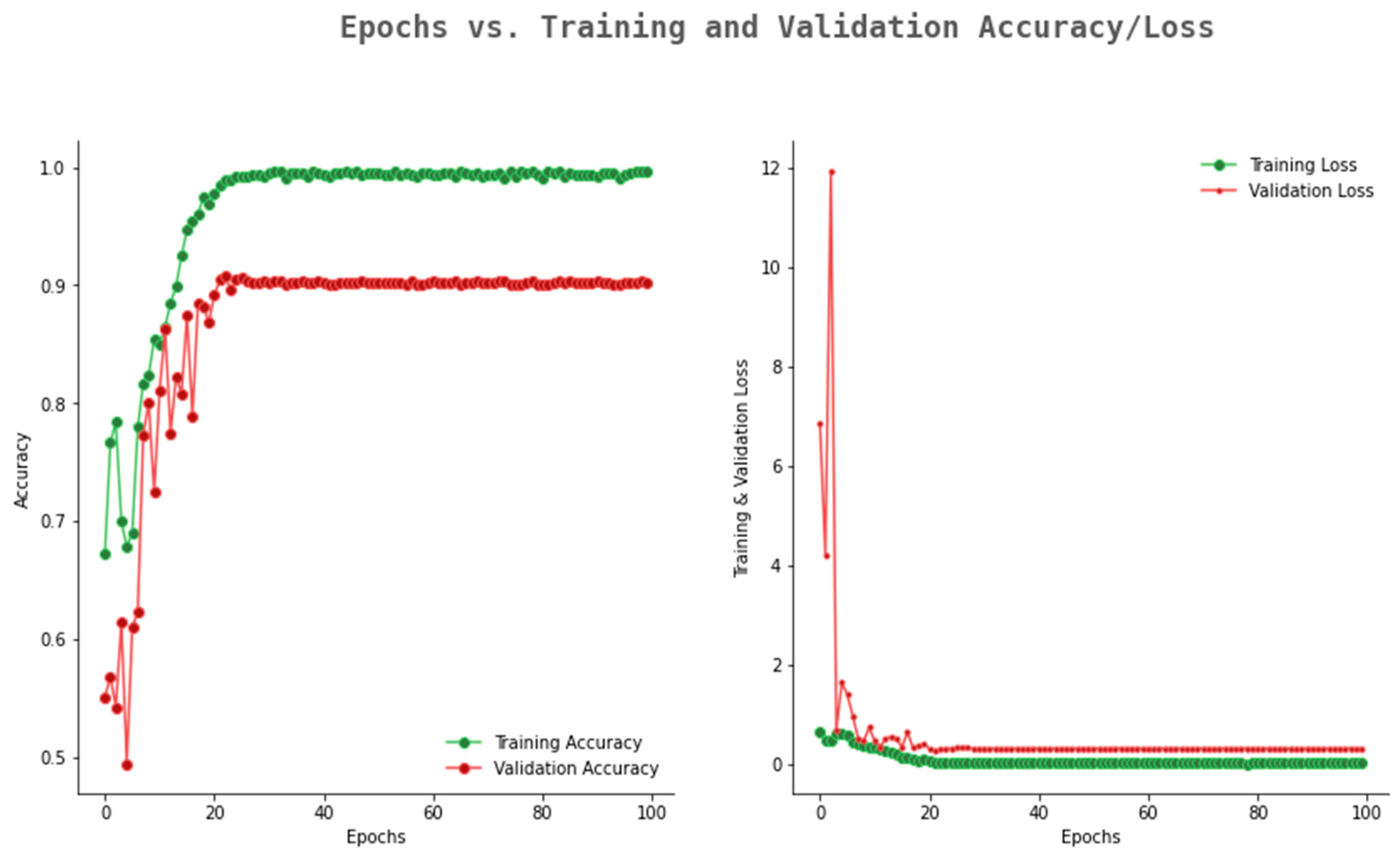
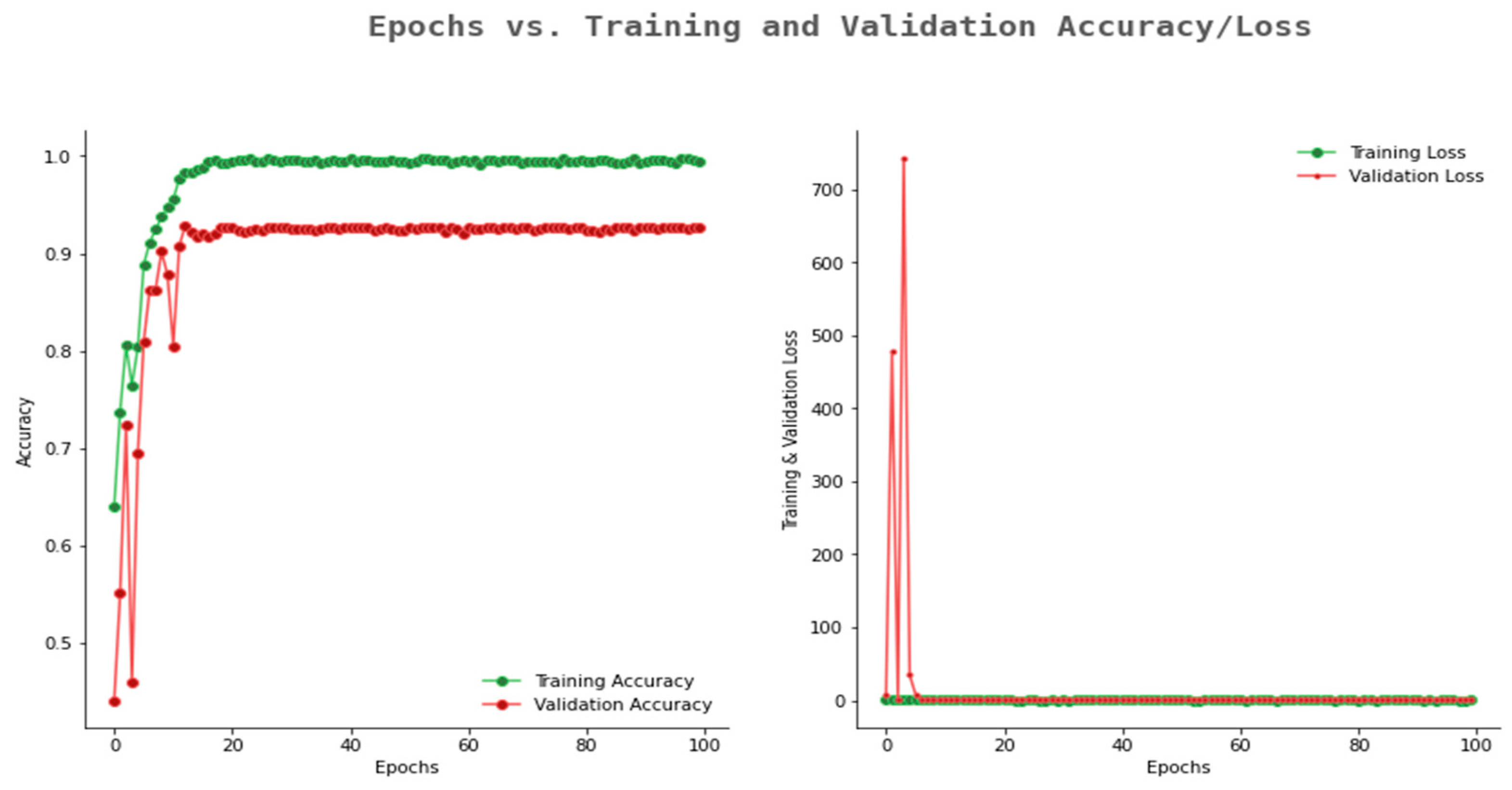
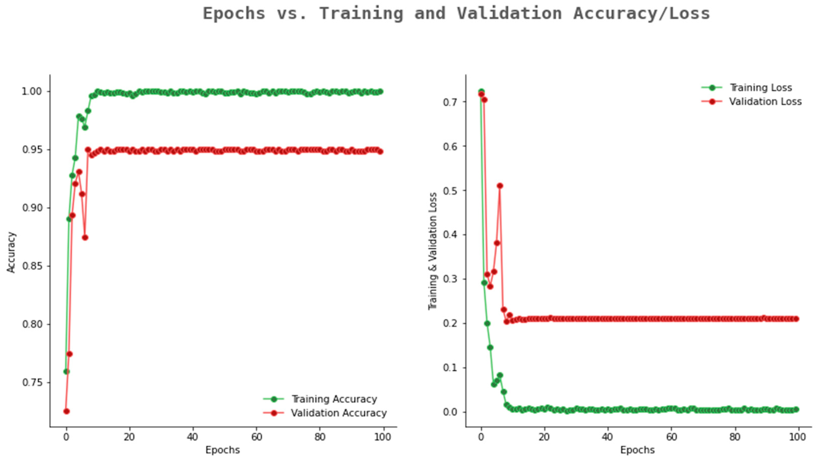
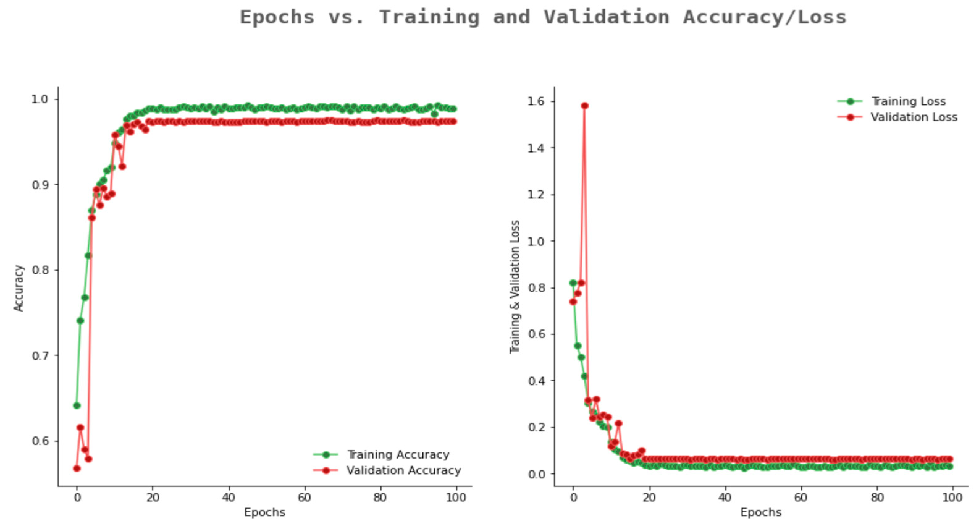
6.2. Result Analysis Using Performance Measure Graph
6.3. Comparative Analysis with Various Models Available in Literature
7. Conclusions
Author Contributions
Funding
Institutional Review Board Statement
Informed Consent Statement
Data Availability Statement
Conflicts of Interest
References
- Borse, V.; Konwar, A.N.; Buragohain, P. Oral cancer diagnosis and perspectives in India. Sens. Int. 2020, 1, 100046. [Google Scholar] [CrossRef] [PubMed]
- Markopoulos, A.K. Current aspects on oral squamous cell carcinoma. Open Dent. J. 2012, 6, 126. [Google Scholar] [CrossRef]
- Bray, F.; Ren, J.-S.; Masuyer, E.; Ferlay, J. Global estimates of cancer prevalence for 27 sites in the adult population in 2008. Int. J. Cancer 2013, 132, 1133–1145. [Google Scholar] [CrossRef]
- Ojansivu, V.; Linder, N.; Rahtu, E.; Pietikäinen, M.; Lundin, M.; Joensuu, H.; Lundin, J. Automated classification of breast cancer morphology in histopathological images. Diagn. Pathol. 2013, 8 (Suppl. S1), S29. [Google Scholar] [CrossRef]
- Sertel, O.; Kong, J.; Shimada, H.; Catalyurek, U.; Saltz, J.; Gurcan, M. Computer-aided prognosis of neuroblastoma on whole-slide images: Classification of stromal development. Pattern Recognit. 2009, 42, 1093–1103. [Google Scholar] [CrossRef]
- Lim, L.A.G.; Maguib, R.N.; Dadios, E.P.; Avila, J.M.C.; Naguib, R.N.G. Implementation of GA-KSOM and ANFIS in the classification of colonic histopathological images. In TENCON 2012 IEEE Region 10 Conference; IEEE: New York, NY, USA, 2012; pp. 1–5. [Google Scholar]
- Li, C.; Zhang, S.; Zhang, H.; Pang, L.; Lam, K.; Hui, C.; Zhang, S. Using the K-nearest neighbor algorithm for the classification of lymph node metastasis in gastric cancer. Comput. Math. Methods Med. 2012, 2012, 876545. [Google Scholar] [CrossRef]
- Hilado, S.D.F.; Lim, L.A.G.; Naguib, R.N.; Dadios, E.P.; Avila, J.M.C. Implementation of wavelets and artificial neural networks in colonic histopathological classification. J. Adv. Comput. Intell. Intell. Inform. 2014, 18, 792–797. [Google Scholar] [CrossRef]
- Deif, M.A.; Attar, H.; Amer, A.; Issa, H.; Khosravi, M.R.; Solyman, A.A.A. A New Feature Selection Method Based on Hybrid Approach for Colorectal Cancer Histology Classification. Wirel. Commun. Mob. Comput. 2022, 2022, 7614264. [Google Scholar] [CrossRef]
- Chen, G.; Zhang, J.; Zhuo, D.; Pan, Y.; Pang, C. Identification of pulmonary nodules via CT images with hierarchical fully convolutional networks. Med. Biol. Eng. Comput. 2019, 57, 1567–1580. [Google Scholar] [CrossRef]
- Cireşan, D.C.; Giusti, A.; Gambardella, L.M.; Schmidhuber, J. Mitosis detection in breast cancer histology images with deep neural networks. In International Conference on Medical Image Computing and Computer-Assisted Intervention; Springer: Berlin/Heidelberg, Germany, 2013; pp. 411–418. [Google Scholar]
- Pavlou, M.; Ambler, G.; Seaman, S.; Guttmann, O.; Elliott, P.; King, M.; Omar, R.Z. How to develop a more accurate risk prediction model when there are few events. BMJ 2015, 351, h3868. [Google Scholar] [CrossRef]
- Su, Y.; Huang, C.; Yin, W.; Lyu, X.; Ma, L.; Tao, Z. Diabetes Mellitus risk prediction using age adaptation models. Biomed. Signal Process. Control. 2023, 80, 104381. [Google Scholar] [CrossRef]
- Wang, Y.; Yao, Q.; Kwok, J.T.; Ni, L.M. Generalizing from a few examples: A survey on few-shot learning. ACM Comput. Surv. 2020, 53, 1–34. [Google Scholar] [CrossRef]
- Shorten, C.; Khoshgoftaar, T.M. A survey on image data augmentation for deep learning. J. Big Data 2019, 6, 1–48. [Google Scholar]
- Krishnan, M.M.R.; Acharya, U.R.; Chakraborty, C.; Ray, A.K. Automated diagnosis of oral cancer using higher order spectra features and local binary pattern: A comparative study. Technol. Cancer Res. Treat. 2011, 10, 443–455. [Google Scholar] [CrossRef] [PubMed]
- Patra, R.; Chakraborty, C.; Chatterjee, J. Textural analysis of spinous layer for grading oral submucous fibrosis. Int. J. Comput. Appl. 2012, 47, 975–8887. [Google Scholar] [CrossRef]
- Driemel, O.; Kunkel, M.; Hullmann, M.; Eggeling, F.V.; Müller-Richter, U.; Kosmehl, H.; Reichert, T.E. Diagnosis of oral squamous cell carcinoma and its precursor lesions. JDDG J. Der Dtsch. Dermatol. Ges. 2007, 5, 1095–1100. [Google Scholar] [CrossRef]
- Rahman, T.; Mahanta, L.; Chakraborty, C.; DAS, A.; Sarma, J. Textural pattern classification for oral squamous cell carcinoma. J. Microsc. 2018, 269, 85–93. [Google Scholar] [CrossRef] [PubMed]
- Rahman, T.Y.; Mahanta, L.B.; Choudhury, H.; Das, A.K.; Sarma, J.D. Study of morphological and textural features for classification of oral squamous cell carcinoma by traditional machine learning techniques. Cancer Rep. 2020, 3, e1293. [Google Scholar] [CrossRef] [PubMed]
- Krishnan, M.M.R.; Venkatraghavan, V.; Acharya, U.R.; Pal, M.; Paul, R.R.; Min, L.C.; Ray, A.K.; Chatterjee, J.; Chakraborty, C. Automated oral cancer identification using histopathological images: A hybrid feature extraction paradigm. Micron 2012, 43, 352–364. [Google Scholar] [CrossRef]
- Krishnan, M.M.R.; Chakraborty, C.; Paul, R.R.; Ray, A.K. Hybrid segmentation, characterization and classification of basal cell nuclei from histopathological images of normal oral mucosa and oral submucous fibrosis. Expert Syst. Appl. 2012, 39, 1062–1077. [Google Scholar] [CrossRef]
- Anuradha, K.; Sankaranarayanan, K. Detection of Oral Tumors using Marker Controlled Segmentation. Int. J. Comp. Appl. 2012, 52, 15–18. [Google Scholar]
- Thomas, B.; Kumar, V.; Saini, S. Texture analysis based segmentation and classification of oral cancer lesions in color images using ANN. In 2013 IEEE International Conference on Signal Processing, Computing and Control (ISPCC); IEEE: New York, NY, USA, 2013; pp. 1–5. [Google Scholar]
- Das, D.K.; Chakraborty, C.; Sawaimoon, S.; Maiti, A.K.; Chatterjee, S. Automated identification of keratinization and keratin pearl area from in situ oral histological images. Tissue Cell 2015, 47, 349–358. [Google Scholar] [CrossRef] [PubMed]
- Das, D.K.; Bose, S.; Maiti, A.K.; Mitra, B.; Mukherjee, G.; Dutta, P.K. Automatic identification of clinically relevant regions from oral tissue histological images for oral squamous cell carcinoma diagnosis. Tissue Cell 2018, 53, 111–119. [Google Scholar] [CrossRef] [PubMed]
- Shi, L.; Liu, W.; Zhang, H.; Xie, Y.; Wang, D. A survey of GPU-based medical image computing techniques. Quant. Imaging Med. Surg. 2012, 2, 188. [Google Scholar]
- Srinidhi, C.L.; Ciga, O.; Martel, A.L. Deep neural network models for computational histopathology: A survey. Med. Image Anal. 2021, 67, 101813. [Google Scholar] [CrossRef]
- Das, N.; Hussain, E.; Mahanta, L.B. Automated classification of cells into multiple classes in epithelial tissue of oral squamous cell carcinoma using transfer learning and convolutional neural network. Neural Netw. 2020, 128, 47–60. [Google Scholar] [CrossRef]
- Panigrahi, S.; Swarnkar, T. Automated Classification of Oral Cancer Histopathology images using Convolutional Neural Network. In 2019 IEEE International Conference on Bioinformatics and Biomedicine (BIBM); IEEE: New York, NY, USA, 2019; pp. 1232–1234. [Google Scholar]
- Panigrahi, S.; Das, J.; Swarnkar, T. Capsule network based analysis of histopathological images of oral squamous cell carcinoma. J. King Saud Univ.-Comput. Inf. Sci. 2020, 34, 4546–4553. [Google Scholar] [CrossRef]
- Karen, S.; Zisserman, A. Very deep convolutional networks for large-scale image recognition. arXiv 2014, arXiv:1409.1556. [Google Scholar]
- Prabhakar, S.K.; Rajaguru, H. Performance analysis of linear layer neural networks for oral cancer classification. In 2017 6th ICT International Student Project Conference (ICT-ISPC); IEEE: New York, NY, USA, 2017; pp. 1–4. [Google Scholar]
- Xi, E. Image feature extraction and analysis algorithm based on multi-level neural network. In 2021 5th International Conference on Computing Methodologies and Communication (ICCMC); IEEE: New York, NY, USA, 2021. [Google Scholar]
- Shrestha, A.; Mahmood, A. Review of deep learning algorithms and architectures. IEEE Access 2019, 7, 53040–53065. [Google Scholar] [CrossRef]
- Li, J.; Song, K. Research on Image Classification Based on Deep Learning. In 2021 IEEE/ACIS 19th International Conference on Computer and Information Science (ICIS); IEEE: New York, NY, USA, 2021; pp. 132–136. [Google Scholar]
- Yousef, R.; Gupta, G.; Yousef, N.; Khari, M. A holistic overview of deep learning approach in medical imaging. Multimed. Syst. 2022, 28, 881–914. [Google Scholar] [CrossRef]
- Alzubaidi, L.; Zhang, J.; Humaidi, A.J.; Al-Dujaili, A.; Duan, Y.; Al-Shamma, O.; Santamaría, J.; Fadhel, M.A.; Al-Amidie, M.; Farhan, L. Review of deep learning: Concepts, CNN architectures, challenges, applications, future directions. J. Big Data 2021, 8, 1–74. [Google Scholar] [CrossRef] [PubMed]
- Bhatt, D.; Patel, C.; Talsania, H.; Patel, J.; Vaghela, R.; Pandya, S.; Modi, K.; Ghayvat, H. CNN variants for computer vision: History, architecture, application, challenges and future scope. Electronics 2021, 10, 2470. [Google Scholar] [CrossRef]
- Rahman, T.Y.; Mahanta, L.B.; Das, A.K.; Sarma, J.D. Histopathological imaging database for oral cancer analysis. Data Brief 2020, 29, 105114. [Google Scholar] [CrossRef] [PubMed]
- Gedraite, E.S.; Hadad, M. Investigation on the effect of a Gaussian Blur in image filtering and segmentation. In Proceedings ELMAR-2011; IEEE: New York, NY, USA, 2011; pp. 393–396. [Google Scholar]
- Kashyap, R. Breast cancer histopathological image classification using stochastic dilated residual ghost model. Int. J. Inf. Retr. Res. (IJIRR) 2022, 12, 1–24. [Google Scholar]
- Nguyen, Q.H.; Ly, H.-B.; Ho, L.S.; Al-Ansari, N.; Van Le, H.; Tran, V.Q.; Prakash, I.; Pham, B.T. Influence of data splitting on performance of machine learning models in prediction of shear strength of soil. Math. Probl. Eng. 2021, 2021, 4832864. [Google Scholar] [CrossRef]
- Qin, X.; Ban, Y.; Wu, P.; Yang, B.; Liu, S.; Yin, L.; Liu, M.; Zheng, W. Improved Image Fusion Method Based on Sparse Decomposition. Electronics 2022, 11, 2321. [Google Scholar] [CrossRef]
- Hu, Z.; Zhao, T.V.; Huang, T.; Ohtsuki, S.; Jin, K.; Goronzy, I.N.; Wu, B.; Abdel, M.P.; Bettencourt, J.W.; Berry, G.J.; et al. The transcription factor RFX5 coordinates antigen-presenting function and resistance to nutrient stress in synovial macrophages. Nat. Metab. 2022, 4, 759–774. [Google Scholar] [CrossRef]
- Zhao, H.; Ming, T.; Tang, S.; Ren, S.; Yang, H.; Liu, M.; Tao, Q.; Xu, H. Wnt signaling in colorectal cancer: Pathogenic role and therapeutic target. Mol. Cancer 2022, 21, 1–34. [Google Scholar] [CrossRef]
- Canesche, M.; Bragança, L.; Neto OP, V.; Nacif, J.A.; Ferreira, R. Google colab cad4u: Hands-on cloud laboratories for digital design. In 2021 IEEE International Symposium on Circuits and Systems (ISCAS); IEEE: New York, NY, USA, 2021; pp. 1–5. [Google Scholar]
- Hicks, S.A.; Strümke, I.; Thambawita, V.; Hammou, M.; Riegler, M.A.; Halvorsen, P.; Parasa, S. On evaluation metrics for medical applications of artificial intelligence. Sci. Rep. 2022, 12, 1–9. [Google Scholar] [CrossRef]
- Gu, S.; Pednekar, M.; Slater, R. Improve image classification using data augmentation and neural networks. SMU Data Sci. Rev. 2019, 2, 1. [Google Scholar]


| Category | Type | Total Quantity | Normal Images | Cancerous Images |
|---|---|---|---|---|
| Category-1 | 100× magnification | 528 | 89 | 439 |
| Category-2 | 400× magnification | 696 | 201 | 495 |
| Total images = | 1224 | 290 | 934 | |
| Category | No of Original OSCC Image | No. of New Images Generated from OSCC Images | No. of Original Non-Cancerous Image | No. of New Images Generated from Non-Cancerous Image |
|---|---|---|---|---|
| Category-1 | 439 | 2634 | 89 | 1869 |
| Category-2 | 495 | 1485 | 201 | 2211 |
| Total | 934 | 4119 | 290 | 4080 |
| Layer | Output Shape | Number of Kernel/Channel | Kernel Size | Stride | Padding | Parameter Generated |
|---|---|---|---|---|---|---|
| Conv2D-1 | 32 | 1 | 1 | 896 | ||
| Maxpooling2D-1 | 32 | 2 | 1 | 0 | ||
| Batch Normalization | 32 | 1 | 1 | 128 | ||
| Conv2D-2 | 32 | 1 | 1 | 9248 | ||
| Maxpooling2D-2 | 32 | 2 | 1 | 0 | ||
| Batch Normalization | 32 | 1 | 1 | 128 | ||
| Conv2D-3 | 64 | 1 | 1 | 18,496 | ||
| Maxpooling2D-3 | 64 | 2 | 1 | 0 | ||
| Conv2D-4 | 64 | 1 | 1 | 36,928 | ||
| Conv2D-5 | 128 | 1 | 1 | 73,856 | ||
| Maxpooling2D-4 | 128 | 2 | 1 | 0 | ||
| Batch Normalization | 128 | 1 | 1 | 512 | ||
| Conv2D-6 | 128 | 1 | 147,584 | |||
| Maxpooling2D-5 | 128 | 2 | 1 | 0 | ||
| Conv2D-7 | 256 | 1 | 1 | 295,168 | ||
| Batch Normalization | 256 | 1 | 1 | 1024 | ||
| Conv2D-8 | 256 | 1 | 1 | 590,080 | ||
| Global Average Pooling-6 | 256 | 4 | 1 | 0 | ||
| Batch normalization | 256 | 1 | 1 | 1024 | ||
| Dense(sigmoid) | 1024 | 1 | 1 | 263,168 | ||
| Batch Normalization | 1024 | 1 | 1 | 4096 | ||
| Flatten | 1024 | 1 | 1 | 0 | ||
| Dropout | 1024 | 1 | 1 | 0 | ||
| Dense(softmax) | 2 | 1 | 1 | 2050 | ||
| Total=1,444,386 |
| Number of Convolution Layers | Kernel Size | Pooling | Activation Function | Optimizer | Epoch | Dropout Rate | Training Accuracy | Validation Accuracy |
|---|---|---|---|---|---|---|---|---|
| 5 | Avg | ReLU | Adam | 10 | 0.1 | 0.812 | 0.782 | |
| 5 | Avg | ReLU | Adam | 50 | 0.2 | 0.812 | 0.772 | |
| 5 | Max | ReLU | Adam | 100 | 0.3 | 0.851 | 0.813 | |
| 6 | Avg | ReLU | Adam | 10 | 0.1 | 0.811 | 0.769 | |
| 6 | Avg | ReLU | Adam | 50 | 0.2 | 0.817 | 0.771 | |
| 6 | Max | ReLU | Adam | 100 | 0.3 | 0.857 | 0.825 | |
| 7 | Max | ReLU | Adam | 10 | 0.1 | 0.887 | 0.850 | |
| 7 | Max | ReLU | Adam | 50 | 0.2 | 0.935 | 0.892 | |
| 7 | Max | ReLU | Adam | 100 | 0.3 | 0.982 | 0.942 | |
| 8 | Max | ReLU | Adam | 10 | 0.1 | 0.992 | 0.955 | |
| 8 | Max | ReLU | Adam | 50 | 0.2 | 0.992 | 0.969 | |
| 8 | Max | ReLU | Adam | 100 | 0.3 | 0.993 | 0.978 |
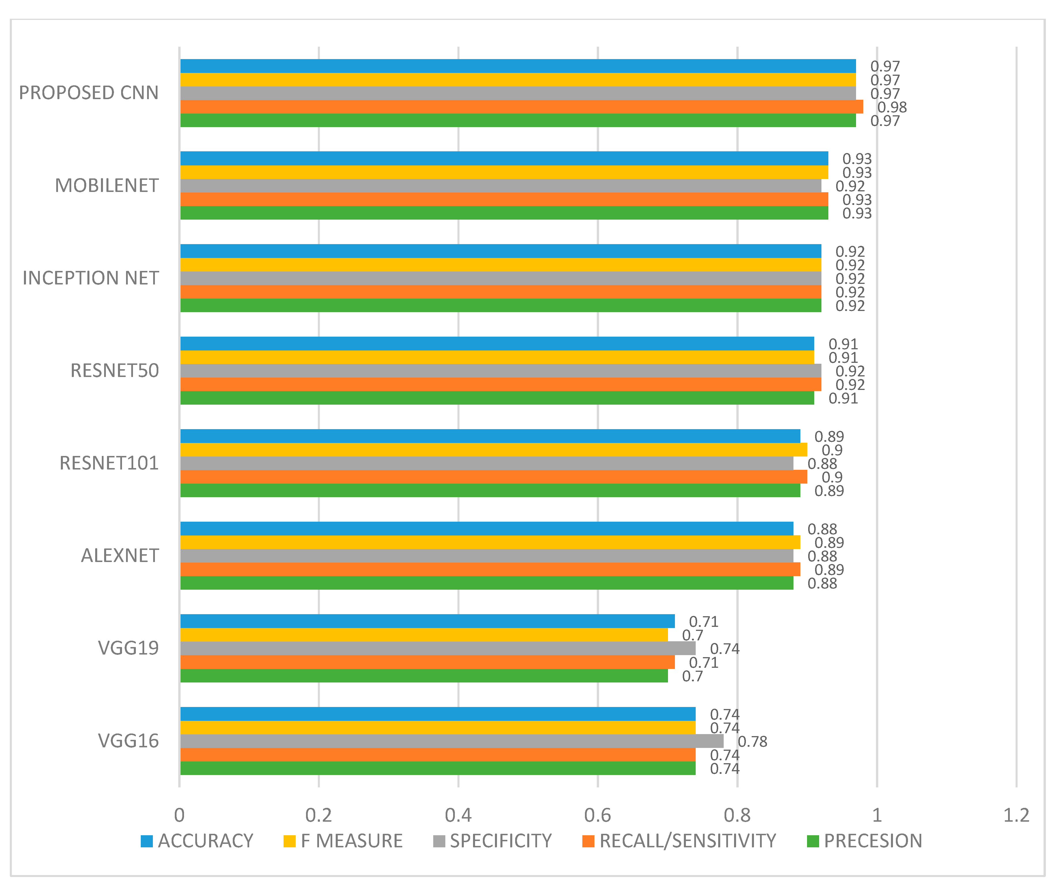
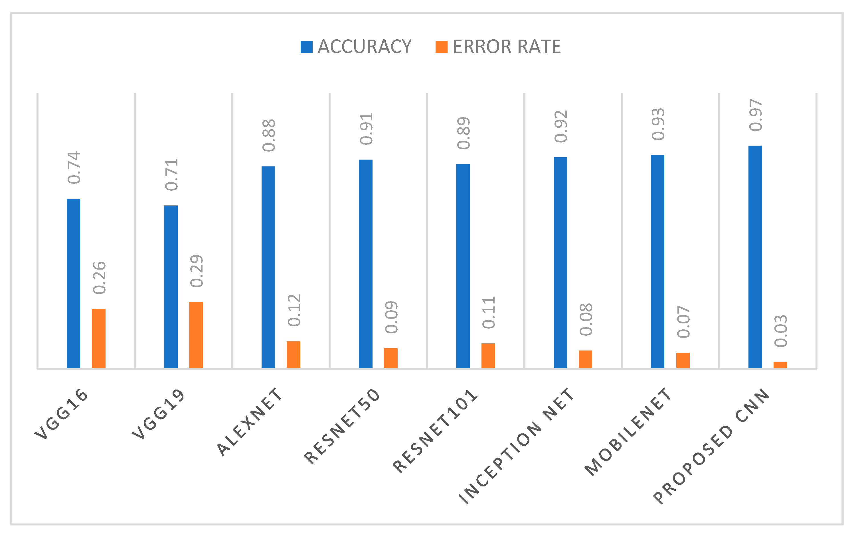
| VGG16 | VGG19 | ALEXNET | RESNET 50 | RESNET 101 | INCEPTION NET | MOBILENET | PROPOSED 10-LAYER CNN | |
|---|---|---|---|---|---|---|---|---|
| Precesion | 0.74 | 0.70 | 0.88 | 0.91 | 0.89 | 0.92 | 0.93 | 0.97 |
| Recall/ Sensitivity | 0.74 | 0.71 | 0.89 | 0.92 | 0.90 | 0.92 | 0.93 | 0.98 |
| Specificity | 0.78 | 0.74 | 0.88 | 0.92 | 0.88 | 0.92 | 0.92 | 0.97 |
| F measure | 0.74 | 0.70 | 0.89 | 0.91 | 0.90 | 0.92 | 0.93 | 0.97 |
| AUC | 0.74 | 0.70 | 0.89 | 0.91 | 0.90 | 0.92 | 0.93 | 0.97 |
| Accuracy | 0.74 | 0.71 | 0.88 | 0.91 | 0.89 | 0.92 | 0.93 | 0.97 |
| Error rate | 0.26 | 0.29 | 0.12 | 0.09 | 0.11 | 0.08 | 0.07 | 0.03 |
| Existing Model in Literature | Method Used | Dataset Used | Accuracy in % |
|---|---|---|---|
| Navarun et al. (2020) [29] | CNN | Histopathological oral cavity images | 97.50 |
| Santisudha et al. (2019) [30] | CNN | Histopathological oral cavity images | 96.77 |
| Santisudha et al. (2020) [31] | Capsule Network | Histopathological oral cavity images | 97.35 |
| Proposed 10-layer CNN model | Customized CNN | Histopathological oral cavity images | 97.82 |
Disclaimer/Publisher’s Note: The statements, opinions and data contained in all publications are solely those of the individual author(s) and contributor(s) and not of MDPI and/or the editor(s). MDPI and/or the editor(s) disclaim responsibility for any injury to people or property resulting from any ideas, methods, instructions or products referred to in the content. |
© 2023 by the authors. Licensee MDPI, Basel, Switzerland. This article is an open access article distributed under the terms and conditions of the Creative Commons Attribution (CC BY) license (https://creativecommons.org/licenses/by/4.0/).
Share and Cite
Das, M.; Dash, R.; Mishra, S.K. Automatic Detection of Oral Squamous Cell Carcinoma from Histopathological Images of Oral Mucosa Using Deep Convolutional Neural Network. Int. J. Environ. Res. Public Health 2023, 20, 2131. https://doi.org/10.3390/ijerph20032131
Das M, Dash R, Mishra SK. Automatic Detection of Oral Squamous Cell Carcinoma from Histopathological Images of Oral Mucosa Using Deep Convolutional Neural Network. International Journal of Environmental Research and Public Health. 2023; 20(3):2131. https://doi.org/10.3390/ijerph20032131
Chicago/Turabian StyleDas, Madhusmita, Rasmita Dash, and Sambit Kumar Mishra. 2023. "Automatic Detection of Oral Squamous Cell Carcinoma from Histopathological Images of Oral Mucosa Using Deep Convolutional Neural Network" International Journal of Environmental Research and Public Health 20, no. 3: 2131. https://doi.org/10.3390/ijerph20032131
APA StyleDas, M., Dash, R., & Mishra, S. K. (2023). Automatic Detection of Oral Squamous Cell Carcinoma from Histopathological Images of Oral Mucosa Using Deep Convolutional Neural Network. International Journal of Environmental Research and Public Health, 20(3), 2131. https://doi.org/10.3390/ijerph20032131