
Environmental Pollution Liability Insurance Pricing and the Solvency of Insurance Companies in China: Based on the Black–Scholes Model


Abstract
1. Introduction
1.1. Research Motivation
1.2. Research Design
1.3. Incremental Contributions
2. Methods and Materials
2.1. Black–Scholes (B-S) Differential Equation
2.2. Multiple Regression
2.3. Data Collection
2.3.1. B-S Calculation of Pricing Model
2.3.2. Pricing of B-S Model of Environmental Liability Insurance
2.4. Data Reduction by Different Companies
2.4.1. Macro-Level
2.4.2. Micro-Level
3. Results and Discussion
3.1. Calculation of Premium Rate of B-S Pricing Model of Environmental Liability Insurance
3.1.1. The First Step Is to Select a Risk-Free Interest Rate
3.1.2. The Second Step Is to Calculate the Volatility
3.1.3. The Third Step Is to Calculate the Insurance Premium Rate
3.2. Main Effect Test
3.2.1. CIC
3.2.2. PICC
3.2.3. API
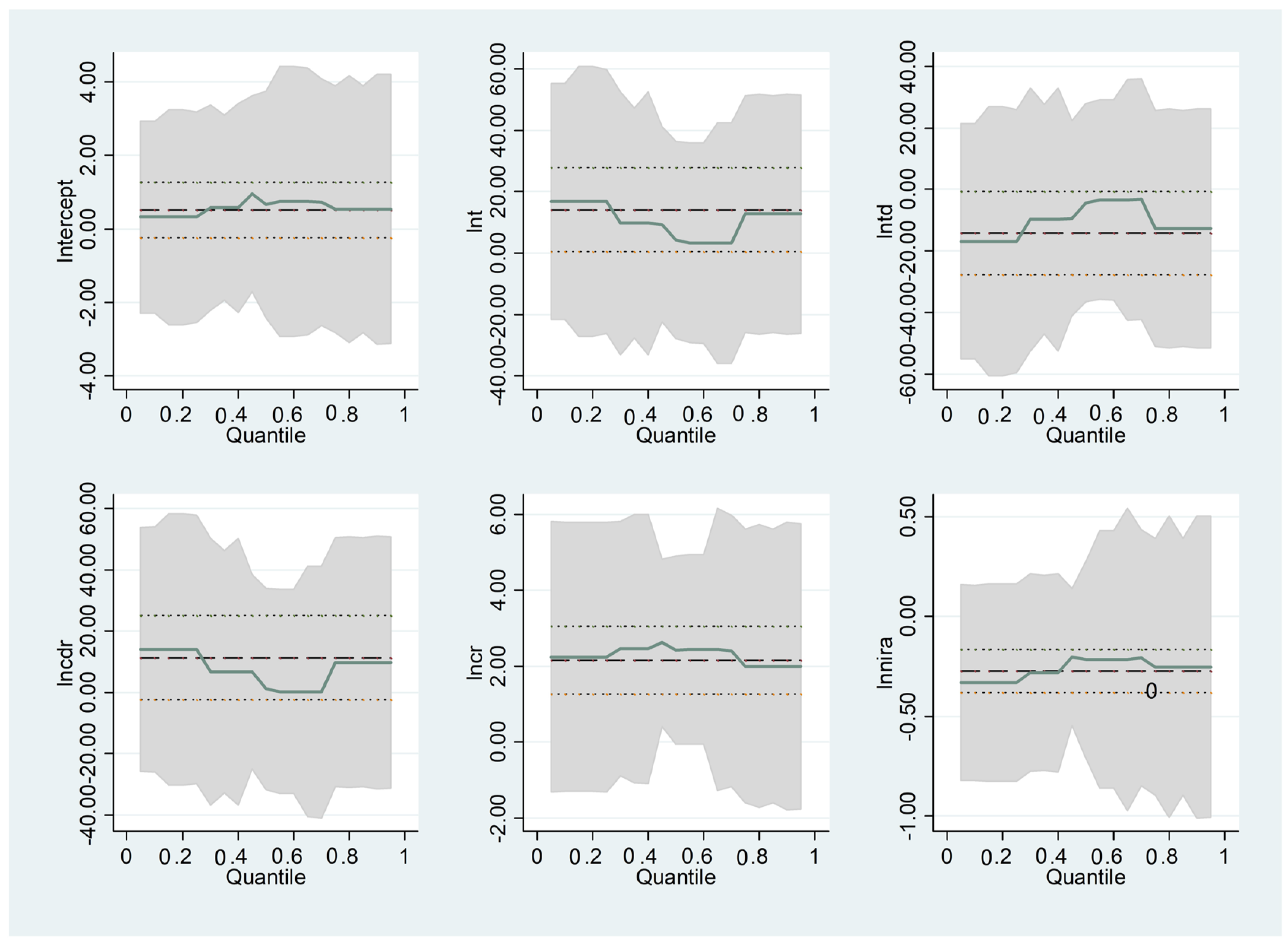
3.3. Robustness Test
4. Conclusions and Recommendations
4.1. Conclusions
4.2. Recommendations
Author Contributions
Funding
Institutional Review Board Statement
Informed Consent Statement
Data Availability Statement
Conflicts of Interest
References
- Shui, B.; Harriss, R.C. The role of CO2 embodiment in US-China trade. Energy Policy 2006, 34, 18. [Google Scholar] [CrossRef]
- Condon, J.B. Climate change and unresolved issue in WTO law. J. Int. Econ. Law 2009, 12, 17. [Google Scholar] [CrossRef]
- Dong, Y.; Whalley, J. Optimal tariff calculations in tariff games with climate change considerations. Appl. Econ. Lett. 2011, 15, 1431–1435. [Google Scholar] [CrossRef]
- Mander, T.; Veenendaal, P. Border tax adjustments and the EU-ETS: A quantitative assessment. Holland: Central Planning Bureau. CPB Doc. 2008, 171, 36. [Google Scholar]
- Feinerman, E.; Plessner, Y.; Dafna, M. Recycled effluent: Should the polluter pay. Am. J. Agric. Econ. 2001, 83, 958–971. [Google Scholar] [CrossRef]
- Erin, E. Dooley, Fifty years later: Clearing the air over the London smog. Environ. Health Perspect. 2002, 110, 748. [Google Scholar]
- Yu, M.; Cruz, J.M.; Li, D.M. The sustainable supply chain network competition with environmental tax policies. Int. J. Prod. Econ. 2019, 217, 218–231. [Google Scholar] [CrossRef]
- Lu, Y.; Wang, Y.; Zhang, W.; Hubacek, K.; Bi, F.; Zuo, J.; Jiang, H.; Zhang, Z.; Feng, K.; Liu, Y.; et al. Provincial air pollution responsibility and environmental tax of China based on interregional linkage indicators. J. Clean. Prod. 2019, 235, 337–347. [Google Scholar] [CrossRef]
- Michael, F.; Grimeaud, D. Financial Assurance Issue of Environmental Liability; Springer-Verlag: Wien, Austria, 2003; pp. 152–153. [Google Scholar]
- Whitmore, A. Compulsory environmental liability insurance as a means of dealing with climate change risk. Energy Policy 2000, 11, 739–741. [Google Scholar] [CrossRef]
- Lockett, N. Environmental Liability Insurance; May Ltd.: Geneva, Switzerland, 1996; p. 19. [Google Scholar]
- Felson, M.; Spaeth, J.L. Community structure and collaborative consumption: A routine activity approach. Am. Behav. Sci. 1978, 21, 4. [Google Scholar] [CrossRef]
- Rifkin, J. The age of access: The new culture of hyper-capitalism where all of life is a paid-for experience. Radic. Teach. 2001, 6, 114. [Google Scholar]
- Botsman, R.; Rogers, R. What’s Mine Is Yours: How Collaborative Consumption Is Changing the Way We Live; Collins: London, UK, 2011; pp. 10–15. [Google Scholar]
- Belk, R. Local government 2035: You are what you can access: Sharing and collaborative consumption. J. Bus. Res. 2015, 67, 1595–1600. [Google Scholar] [CrossRef]
- Yan, F.; Arthur, P.J.; Lu, Y.; He, G.; Van Koppen, C.S.A. Environmental pollution liability insurance in China: Compulsory or voluntary. J. Clean. Prod. 2014, 5, 211–219. [Google Scholar]
- Thomas, F. Welcome to the Sharing Economy; The New York Times: Manhattan, NY, USA, 2013. [Google Scholar]
- Dong, Q. Research on the energy-saving and revenue sharing strategy of ESCOs under the uncertainty of the value of Energy Performance Contracting Projects. Energy Policy 2014, 73, 710–721. [Google Scholar]
- Lee, P. Risks in energy performance contracting (EPC) projects. Energy Build. 2015, 92, 116–127. [Google Scholar] [CrossRef]
- Li, Y. AHP-fuzzy evaluation on financing bottleneck in energy performance contracting in China. Energy Procedia 2011, 14, 121–126. [Google Scholar] [CrossRef]
- Polzin, F. What encourages local authorities to engage with energy performance contracting for retrofitting? Evidence from German municipalities. Energy Policy 2016, 94, 317–330. [Google Scholar] [CrossRef]
- Xiaohong, Z. Problem and countermeasure of energy performance Contracting in China. Energy Procedia 2010, 5, 1377–1381. [Google Scholar] [CrossRef]
- Deng, Q. Strategic design of cost savings guarantee in energy performance contracting under uncertainty. Appl. Energy 2014, 139, 68–80. [Google Scholar] [CrossRef]
- Zhang, S.; Mendelsohn, R.; Cai, W.; Cai, B.; Wang, C. Incorporating health impacts into a differentiated pollution tax rate system: A case study in the Beijing-Tianjin-Hebei region in China. J. Environ. Manag. 2019, 15, 250. [Google Scholar] [CrossRef]
- Gilchrit, T. Insurance coverage for pollution liability in the United States and the United Kingdom: Covering troubled waters. Hein Online 1991, 23, 1. [Google Scholar]
- Maggie, J. A bumpy road leading to a bright prospect. Asia Insur. Rev. 2012, 1, 82–83. [Google Scholar]
- OECD. Environmental Risks and Insurance; OECD Home: Paris, France, 2003; p. 5. [Google Scholar]
- Merrifield, J. A general equilibrium analysis of the insurance bonding approach to pollution threats. Ecol. Econ. 2002, 1, 20. [Google Scholar] [CrossRef]
- Ackermana, F.; Ishikawab, M.; Suga, M. The carbon content of Japan-US trade. Energy Policy 2007, 35, 4455–4462. [Google Scholar] [CrossRef]
- Syunkova. WTO compatibility of four categories of US climate change policy. Natl. Foreign Trade Counc. Rep. 2007, 5, 12–13. [Google Scholar]
- Richardson, B.J. Mandating environmental liability insurance. Duke Environ. Law Policy Forum 2002, 15, 293–330. [Google Scholar]
- Dressler, L.; Hanappi, T.; van Dender, K. Unintended technology-bias in corporate income taxation. OECD Tax. Work. Pap. 2018, 37, 9f4a34ff-en. [Google Scholar]
- Choi, T.M. Multi-period risk minimization purchasing models for fashion products with interest rate, budget, and profit target considerations. Ann. Oper. Res. 2016, 237, 77–98. [Google Scholar] [CrossRef]
- Dong, Y.; Walley, J. Carbon motivated regional trade arrangements: Analytics and simulations. Econ. Model. 2011, 28, 2783–2792. [Google Scholar] [CrossRef]
- Ohno, T. Efficiency of environmental taxes in open and closed economics. Stud. Reg. Sci. 2014, 44, 167–180. [Google Scholar] [CrossRef]
- Lockwood, B.; Whalley, J. Carbon-motivated border tax adjustments: Old wine in green bottles? World Econ. 2010, 33, 810–819. [Google Scholar] [CrossRef]
- Ekins, P. Resource Productivity, Environmental Tax Reform and Sustainable Growth in Europe; Anglo-German Foundation: London, UK, 2009. [Google Scholar]
- Peterson, J.M. Estimating an Effluent Charge: The Reserve Mining Case; University of Wisconsin Press: Madison, WI, USA, 1977; pp. 328–341. [Google Scholar]
- Othman, J. Carbon and energy taxation for CO2 mitigation: A CGE model of the Malaysia. Environ. Dev. Sustain. 2017, 19, 239–262. [Google Scholar]
- Terkla, D. The efficiency value of effluent tax revenues. J. Environ. Econ. Manag. 1984, 11, 107–123. [Google Scholar] [CrossRef]
- Brenner, M.; Riddle, M.; Boyce, J.K. A Chinese sky trust: Distributional impacts of carbon charges am revenue recycling China. Energy Policy 2007, 35, 1771–1784. [Google Scholar] [CrossRef]
- Halkos, G.E.; Paizanos, E.A. The effect of government expenditure on the environment: An empirical investigation. Ecol. Econ. 2013, 91, 48–56. [Google Scholar] [CrossRef]
- Hu, X.; Liu, J.; Yang, H.; Meng, J.; Wang, X.; Ma, J.; Tao, S. Impacts of potential China’s environmental protection tax reforms on provincial air pollution emissions and economy. Earths Future 2020, 8, 4. [Google Scholar] [CrossRef]
- Karydas, C.; Zhang, L. Green tax reform, endogenous innovation and the growth dividend. J. Environ. Econ. Manag. 2019, 97, 158–181. [Google Scholar] [CrossRef]
- Fan, X.; Li, X.; Yin, J. Impact of environmental tax on green development: A nonlinear dynamical system analysis. PLoS ONE 2019, 14, 1–23. [Google Scholar] [CrossRef]
- Hamaguchi, Y. Dynamic analysis of bribery firms’ environmental tax evasion in an emissions trading market. J. Macroecon. 2020, 63, 103169. [Google Scholar] [CrossRef]
- Bovenberg, A.; de Mooij, L.; Ruu, A. Environmental levies and distortionary taxes: Comment. Am. Econ. Rev. 1997, 87, 245–251. [Google Scholar]
- Li, K.; Liu, C. Construction of carbon finance system and promotion of environmental finance Innovation in China. Energy Procedia 2011, 5, 1065–1072. [Google Scholar]
- Wang, N.; Chang, Y.-C. The development of policy instruments in supporting low-carbon governance in China. Renew. Sustain. Energy Rev. 2014, 35, 126–135. [Google Scholar] [CrossRef]
- Khanna, N.; Fridley, D.; Hong, L. China’s pilot low-carbon city initiative: A comparative assessment of national goals and local plans. Sustain. Cities Soc. 2014, 12, 110–121. [Google Scholar] [CrossRef]
- Zhang, B.; Yang, Y.; Bi, J. Tracking the implementation of green credit policy in China: Top-down perspective and bottom-up reform. J. Environ. Manag. 2011, 92, 1321–1327. [Google Scholar] [CrossRef]
- Carraro, C.; Favero, A.; Massetti, E. Investments and public finance in a green, low carbon, economy. Energy Econ. 2012, 34, 15–28. [Google Scholar] [CrossRef]
- Liu, J.; Shen, Z. Low carbon finance: Present situation and future development in China. Energy Procedia 2011, 5, 214–218. [Google Scholar]
- David, W. Clean development mechanism (CDM) after the first commitment period: Assessment of the world’s portfolio and the role of Latin America. Renew. Sustain. Energy Rev. 2015, 41, 1176–1189. [Google Scholar]
- Zhao, Z.-Y.; Li, Z.-W.; Xia, B. The impact of the CDM (clean development mechanism) on the cost price of wind power electricity: A China study. Energy 2014, 1, 179–185. [Google Scholar] [CrossRef]
- Kerchner, C.D.; Keeton, W.S. California’s regulatory forest carbon market: Viability for northeast landowners. For. Policy Econ. 2015, 50, 70–81. [Google Scholar] [CrossRef]
- Yang, R.; Zhang, R. Environmental pollution liability insurance and corporate performance: Evidence from China in the perspective of green development. Int. J. Environ. Res. Public Health 2022, 19, 12089. [Google Scholar] [CrossRef]


| Unit: CNY 100 Million | 2007 | 2008 | 2009 | 2010 | 2011 | 2012 | 2013 | 2014 | 2015 | 2016 |
|---|---|---|---|---|---|---|---|---|---|---|
| Liability insurance Premium | 66.6 | 81.75 | 92.2 | 115.9 | 148.01 | 183.77 | 216.63 | 253.3 | 301.8 | 362.4 |
| Liability insurance compensate | 26.25 | 33.08 | 38.9 | 44 | 57.07 | 75.14 | 89.21 | 107.72 | 129.3 | 166.23 |
| Unit: CNY 10,000 | 2007 | 2008 | 2009 | 2010 | 2011 | 2012 | 2013 | 2014 | 2015 | 2016 |
|---|---|---|---|---|---|---|---|---|---|---|
| Liability insurance compensate | 2529.6 | 503.39 | 591.96 | 669.57 | 868.46 | 1143.4 | 1357.5 | 1639.2 | 1967.6 | 2529.6 |
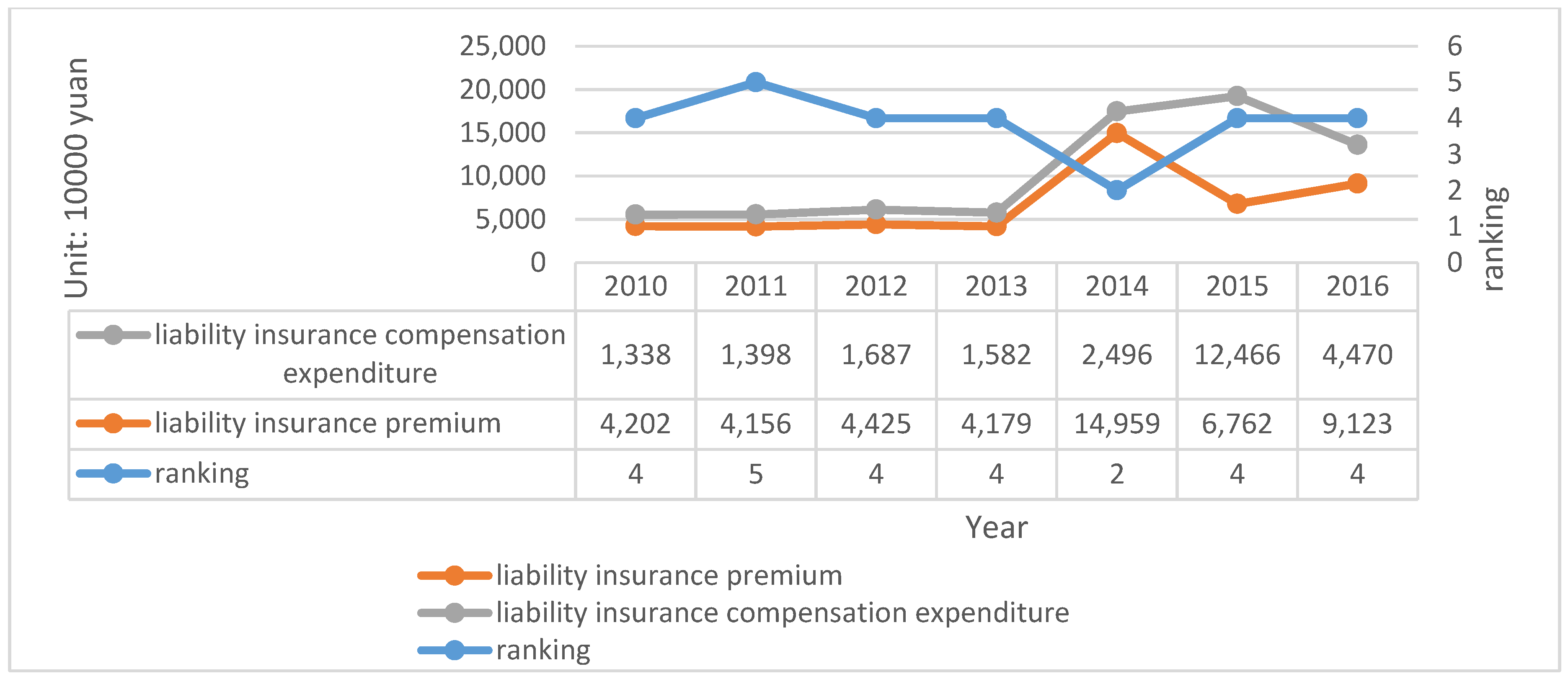
| Unit: CNY 10,000 | 2007 | 2008 | 2009 | 2010 | 2011 | 2012 | 2013 | 2014 | 2015 | 2016 |
|---|---|---|---|---|---|---|---|---|---|---|
| Liability insurance premium | 43.94 | 55.37 | 65.12 | 73.65 | 95.53 | 125.78 | 149.33 | 180.31 | 216.44 | 278.25 |
| Unit: CNY 10,000 | 2007 | 2008 | 2009 | 2010 | 2011 | 2012 | 2013 | 2014 | 2015 | 2016 |
|---|---|---|---|---|---|---|---|---|---|---|
| Liability insurance premium | 63.45 | 76.76 | 86.65 | 94.09 | 117.16 | 148.09 | 168.78 | 195.65 | 225.46 | 278.25 |
| VAR00001 | ||
|---|---|---|
| N | 10 | |
| Normal Parameters a,b | Mean | 145.4340 |
| Std. Deviation | 71.06075 | |
| Most Extreme Differences | Absolute | 0.165 |
| Positive | 0.165 | |
| Negative | −0.124 | |
| Test Statistic | 0.165 | |
| Asymp. Sig. (2-tailed) | 0.200 | |
| Year | 2012 | 2013 | 2014 | 2015 | 2016 | 2017 |
|---|---|---|---|---|---|---|
| Solvency adequacy ratio | 167% | 166.86% | 171.27% | 163.94% | 290.61% | 300.86% |
| Unit: CNY 1000 | 2012 | 2013 | 2014 | 2015 | 2016 | 2017 |
|---|---|---|---|---|---|---|
| Total Asset | 32,774,662 | 37,920,228 | 42,503,286 | 53,034,399 | 59,756,316 | 69,210,296 |
| Total Debt | 25,785,128 | 29,968,904 | 32,035,899 | 39,880,522 | 46,229,646 | 54,550,658 |
| Capital debt ratio | 78.67% | 79.03% | 75% | 75.19% | 77.36% | 78.81% |
| Claim ratio | 38.83% | 36.87% | 39.25% | 35.48% | 40.31% | 43.66% |
| Net interest rate on assets | 6.66% | 3% | 4.69% | 4.61% | 1.47% | 1.86% |
| Year | 2012 | 2013 | 2014 | 2015 | 2016 | 2017 |
|---|---|---|---|---|---|---|
| Solvency adequacy ratio | 175% | 180% | 239% | 226% | 287% | 278% |
| Unit: CNY 1000 | 2012 | 2013 | 2014 | 2015 | 2016 | 2017 |
|---|---|---|---|---|---|---|
| Total Asset | 290,424 | 319,424 | 366,130 | 420,420 | 475,949 | 524,566 |
| Total Debt | 244,974 | 261,920 | 280,355 | 311,469 | 356,637 | 391,452 |
| Capital debt ratio | 84.35% | 81.99% | 76.57% | 74.08% | 74.93% | 74.62% |
| Claim ratio | 44.58% | 42.73% | 44.56% | 44.47% | 47% | 44.99% |
| Net interest rate on assets | 3.58% | 3.30% | 4.12% | 5.19% | 3.78% | 3.77% |
| Year | 2010 | 2011 | 2012 | 2013 | 2014 | 2015 | 2016 |
|---|---|---|---|---|---|---|---|
| Solvency adequacy ratio | 146% | 102% | 441% | 293% | 202% | 210% | 514% |
| Unit: CNY 1000 | 2010 | 2011 | 2012 | 2013 | 2014 | 2015 | 2016 |
|---|---|---|---|---|---|---|---|
| Total Asset | 198,752 | 250,982 | 365,561 | 364,060 | 396,572 | 361,251 | 545,575 |
| Total Debt | 146,200 | 221,600 | 234,725 | 235,325 | 271,347 | 246,375 | 276,022 |
| Capital Debt Ratio | 73.55% | 88% | 64% | 64% | 68% | 68.20% | 50.59% |
| Claim Ratio | 31.84% | 33.63% | 38.12% | 37.85% | 16.68% | 184% | 48.99% |
| Net Interest Rate on Assets | −3.56% | −9.21% | 0.09% | 0.08% | −2.66% | −2.68% | −8.19% |
| Df | SS | MS | F | Significance F | |
|---|---|---|---|---|---|
| Regression Analysis | 4 | 0.4256 | 0.1064 | 10.31 | 0.2290 |
| Residual | 1 | 0.0103 | 0.0103 | ||
| Total | 5 | 0.4359 |
| Variables | SAR 1 | Standard Error | T |
|---|---|---|---|
| TA 2 | 0.2929 *** | 0.0414 | 7.07 |
| TD 3 | - | - | - |
| CDR 4 | 0.0449 | 1.0892 | 0.04 |
| CR 5 | 1.8823 *** | 0.4320 | 4.36 |
| NIRA 6 | −0.1744 *** | 0.0372 | −4.69 |
| Constant | −3.2878 | - | - |
| R-squared | 0.9763 | ||
| Adjusted R-squared | 0.8816 |
| Df | SS | MS | F | Significance F | |
|---|---|---|---|---|---|
| Regression Analysis | 5 | 1.2952 | 0.2590 | 26.24367 | 0.1471 |
| Residual | 1 | 0.0099 | 0.0099 | ||
| Total | 6 | 1.3051 |
| Variables | SAR 1 | Standard Error | T |
|---|---|---|---|
| TA 2 | 9.0461 *** | 2.7400 | 3.2988 |
| TD 3 | −0.0001 *** | 3.8400 | −3.2292 |
| CDR 4 | 19.6514 *** | 8.6160 | 2.2808 |
| CR 5 | 8.9803 * | 4.6747 | 1.9210 |
| NIRA 6 | −56.4684 *** | 15.9622 | −3.5376 |
| Constant | −12.7481 * | 7.1748 | −1.7768 |
| R-squared | 0.9924 | ||
| Adjusted R-squared | 0.9546 |
| Df | SS | MS | F | Significance F | |
|---|---|---|---|---|---|
| Regression Analysis | 5 | 13.4697 | 2.6939 | 4.4926 | 0.3431 |
| Residual | 1 | 0.5996 | 0.5996 | ||
| Total | 6 | 14.0693 |
| Variables | SAR 1 | Standard Error | T |
|---|---|---|---|
| TA 2 | 1.6856 ** | 8.6000 | 1.9605 |
| TD 3 | −2.2843 * | 1.1800 | −1.9283 |
| CDR 4 | 91.1216 * | 52.5091 | 1.7353 |
| CR 5 | 0.1527 | 0.6198 | 0.2464 |
| NIRA 6 | −90.3570 * | 48.4435 | 1.8652 |
| Constant | −62.5330 * | 37.1771 | −1.6820 |
| R-squared | 0.9574 | ||
| Adjusted R-squared | 0.7744 |
| (1) | (2) | (3) | (4) | |
|---|---|---|---|---|
| SAR 1 OLS | SAR 1 QR_10 | SAR 1 QR_50 | SAR 1 QR_90 | |
| TA 2 | 14.22 ** (5.565) | 16.87 *** (0.000) | 4.358 * (25.94) | 12.73 *** (2.273) |
| TD 3 | −14.19 ** (5.568) | −16.83 *** (0.000) | −4.313 * (25.96) | −12.70 *** (2.275) |
| CDR 4 | 11.29 * (5.604) | 13.99 *** (0.000) | 1.044 * (25.56) | 9.795 *** (2.371) |
| CR 5 | 2.162 *** (0.366) | 2.243 *** (3.52) | 2.424 * (1.427) | 1.997 *** (0.115) |
| NIRA 6 | −0.274 *** (0.0442) | −0.332 *** (3.98) | −0.217 * (0.142) | −0.253 *** (0.0163) |
| Time control | YES | YES | YES | YES |
| Individual control | YES | YES | YES | YES |
| _cons | 0.524 | 0.319 *** | 0.662 | 0.539 *** |
Disclaimer/Publisher’s Note: The statements, opinions and data contained in all publications are solely those of the individual author(s) and contributor(s) and not of MDPI and/or the editor(s). MDPI and/or the editor(s) disclaim responsibility for any injury to people or property resulting from any ideas, methods, instructions or products referred to in the content. |
© 2023 by the authors. Licensee MDPI, Basel, Switzerland. This article is an open access article distributed under the terms and conditions of the Creative Commons Attribution (CC BY) license (https://creativecommons.org/licenses/by/4.0/).
Share and Cite
Chen, S.; Yang, J. Environmental Pollution Liability Insurance Pricing and the Solvency of Insurance Companies in China: Based on the Black–Scholes Model. Int. J. Environ. Res. Public Health 2023, 20, 1630. https://doi.org/10.3390/ijerph20021630
Chen S, Yang J. Environmental Pollution Liability Insurance Pricing and the Solvency of Insurance Companies in China: Based on the Black–Scholes Model. International Journal of Environmental Research and Public Health. 2023; 20(2):1630. https://doi.org/10.3390/ijerph20021630
Chicago/Turabian StyleChen, Shuai, and Jiameng Yang. 2023. "Environmental Pollution Liability Insurance Pricing and the Solvency of Insurance Companies in China: Based on the Black–Scholes Model" International Journal of Environmental Research and Public Health 20, no. 2: 1630. https://doi.org/10.3390/ijerph20021630
APA StyleChen, S., & Yang, J. (2023). Environmental Pollution Liability Insurance Pricing and the Solvency of Insurance Companies in China: Based on the Black–Scholes Model. International Journal of Environmental Research and Public Health, 20(2), 1630. https://doi.org/10.3390/ijerph20021630