
Impact of Regional Mobility on Air Quality during COVID-19 Lockdown in Mississippi, USA Using Machine Learning


Abstract
1. Introduction
2. Materials and Methods
3. Results
3.1. Time Series Study and Results
- 3.1.1. Time series study of air pollutants
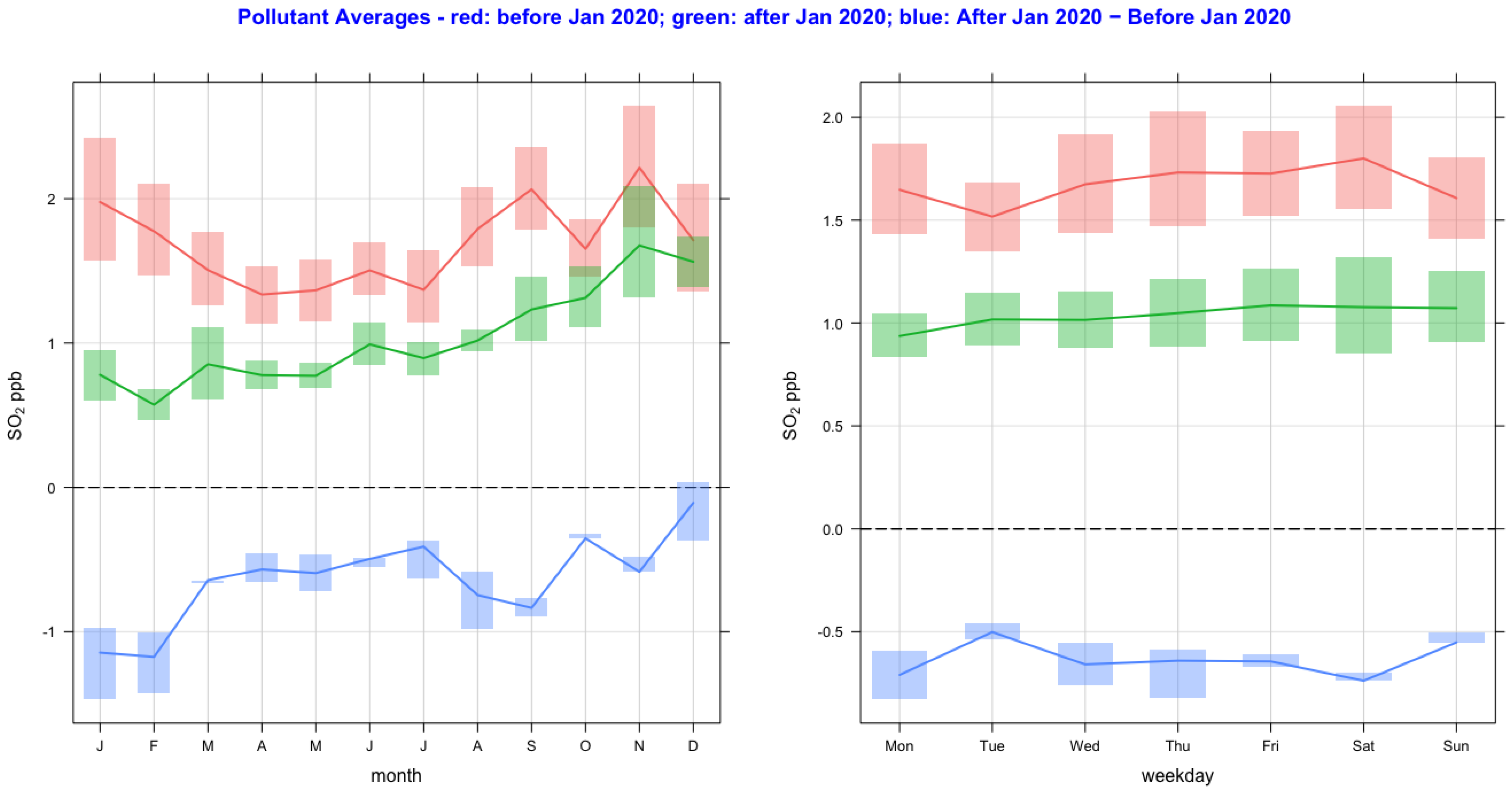
- 3.1.2. Monthly and day-of-the-week variations of air pollutants
- 3.1.3. Time series study of weather
- 3.1.4. Time series study of mobility in MS, 2020
3.1.1. Time Series Study of Air Pollutants
3.1.2. Monthly and Day-of-the-Week Averages of Air Quality
3.1.3. Time Series Study of Meteorological Trends
3.1.4. Mobility: Time Series Study and Results
3.2. Machine Learning Modeling: Business as Usual Scenario Model
- Install and run the packages in R studio [40].
- Load and run the data set for each pollutant and the independent variables.
- Features or independent variables.
- Meteorological variables—temperature, humidity, pressure, wind speed, wind direction, and precipitation.
- Temporal variables—year, month, day, weekday, season.
- Target variable—pollutant concentration.
- Run the random forest model for training and create a meteorological normalized trend.
- Define the training data set period.
- Split the data and the training set; the test is for validation.
- Input features—meteorological and temporal variables.
- Run the RF model using weather normalization.
- ii.
- For each day, resample the meteorological explanatory variables by repeating a certain number of times (say 300).
- iii.
- Aggregate the predicted values from each iteration to obtain the meteorological normalized concentration.
- iv.
- The estimated values represent the emission changes rather than the changes due to meteorological effects.
- v.
- Repeat resampling for every day in the data set.
- Set the hyper-parameters of the model.
- Check the model performance on the test part of the training set.
- Plot variable importance and decide which variables are more important, and remove insignificant variables if required.
- Run the model prediction and check if the model has suffered from overfitting.
- Check for partial dependencies and remove missing variables.
- Run the weather-normalized and trained RF model on the test data set (lockdown period) to obtain the predicted values of the pollutant concentrations.
- Collect the observed and predicted pollutant values; compute the pollutant change due to the lockdown, and plot for visualization.
4. Discussion
5. Conclusions
Author Contributions
Funding
Conflicts of Interest
References
- CDC Air Quality. Available online: https://www.cdc.gov/air/pollutants.htm#:~:text=These%20six%20pollutants%20are%20carbon,matter)%2C%20and%20sulfur%20oxides (accessed on 29 October 2022).
- EPA Air Quality. Available online: https://www.epa.gov/criteria-air-pollutants (accessed on 29 October 2022).
- CDC. Air Quality, and Health. Available online: https://www.cdc.gov/air/particulate_matter.html (accessed on 30 October 2022).
- EPA Asthma. Available online: https://www.epa.gov/asthma (accessed on 30 October 2022).
- WHO. Air Pollution and Health. Available online: https://www.who.int/data/gho/data/themes/topics/indicator-groups/indicator-group-details/GHO/ambient-air-pollution#:~:text=Air%20pollution%20is%20associated%20with,(COPD)%20and%20cardiovascular%20diseases (accessed on 1 November 2022).
- Zhou, X.; Josey, K.; Kamareddine, L.; Caine, M.C.; Dominici, F. Excess of COVID-19 cases and deaths due to fine particulate matter exposure during the 2020 wildfires in the United States. Sci. Adv. 2021, 7, eabi8789. [Google Scholar] [CrossRef] [PubMed]
- Yao, Y.; Pan, J.; Liu, Z.; Meng, X.; Wang, W.; Kan, H.; Wang, W. Temporal association between particulate matter pollution and case fatality rate of COVID-19 in Wuhan. Environ. Res. 2020, 189, 109941. [Google Scholar] [PubMed]
- WHO Declaring COVID-19 Pandemic. Available online: https://www.who.int/director-general/speeches/detail/who-director-general-s-opening-remarks-at-the-media-briefing-on-covid-19---11-march-2020 (accessed on 1 October 2021).
- COVID-19 Incidence World-Meter. Available online: https://www.worldometers.info/coronavirus/#countries (accessed on 1 November 2021).
- COVID-19 and WHO. Available online: https://www.who.int/emergencies/diseases/novel-coronavirus-2019?adgroupsurvey={adgroupsurvey}&gclid=Cj0KCQjwnvOaBhDTARIsAJf8eVMC_zdamVB_ZpNRu-gGtpqhw4a9c09-zjHE9pNVe-cwxCaBpJbeQdQaAqCJEALw_wcB (accessed on 28 October 2022).
- Lockdown Timeline CDC. Available online: https://www.cdc.gov/museum/timeline/covid19.html (accessed on 28 October 2022).
- World Data Lockdown Measures. Available online: https://ourworldindata.org/policy-responses-covid (accessed on 28 October 2022).
- Onyeaka, H.; Anumudu, C.K.; Al-Sharify, Z.T.; Egele-Godswill, E.; Mbaegbu, P. COVID-19 pandemic: A review of the global lockdown and its far-reaching effects. Sci. Prog. 2021, 104, 00368504211019854. [Google Scholar] [CrossRef]
- Lewis, D. What scientists have learnt from COVID lockdowns. Nature 2022, 609, 236–239. [Google Scholar] [CrossRef]
- Connerton, P.; de Assunção, J.V.; de Miranda, M.R.; Slovic, A.D.; Pérez-Martínez, P.J.; Helena Ribeiro, H. Air Quality during COVID-19 in Four Megacities: Lessons and Challenges for Public Health. Int. J. Environ. Res. Public Health 2020, 17, 5067. [Google Scholar] [CrossRef] [PubMed]
- Venter, Z.S.; Aunan, K.; Chowdhury, S.; Lelieveld, J. COVID-19 lockdowns cause global air pollution declines. Earth Atmos. Planet. Sci. 2020, 117, 18984–18990. [Google Scholar] [CrossRef]
- Sarmadi, M.; Rahimi, S.; Rezaei, M.; Sanaei, D.; Dianatinasab, M. Air quality index variation before and after the onset of COVID-19 pandemic: A comprehensive study on 87 capital, industrial and polluted cities of the world. Environ. Sci. Eur. 2021, 33, 134. [Google Scholar] [CrossRef]
- Shi, Z.; Song, C.; Liu, B.; Lu, G.; Xu, J.; Van Vu, T.; Elliott, R.J.; Li, W.; Bloss, W.J.; Harrison, R.M. Abrupt but smaller than expected changes in surface air quality attributable to COVID-19 lockdowns. Sci. Adv. 2021, 7, eabd6696. [Google Scholar] [CrossRef]
- Jiang, Z.; Shi, H.; Zhao, B.; Gu, Y.; Zhu, Y.; Miyazaki, K.; Zhang, Y.; Bowman, K.W.; Sekiya, T.; Kuo-Nan Liou, K.N. Modeling the Impact of COVID-19 on Air Quality in Southern California: Implications for Future Control Policies. Atmos. Chem. Phys. 2021, 21, 8693–8708. [Google Scholar] [CrossRef]
- Campbell, P.C.; Tong, D.; Tang, Y.; Baker, B.; Lee, P.; Saylor, R.; Stein, A.; Ma, S.; Lamsal, L.; Qu, Z. Impacts of the COVID-19 economic slowdown on ozone pollution in the U.S. Atmos. Environ. 2021, 264, 118713. [Google Scholar] [CrossRef]
- Hammer, M.S.; Donkelaar, A.V.; Martin, V.R.; Mcduffie, E.; Lyapustin, A.; Sayer, A.M.; Hsu, N.C.; Levy, R.C.; Garay, M.J.; Kahn, R.A. Effects of COVID-19 lockdowns on fine particulate matter concentrations. Sci. Adv. 2021, 7, eabg7670. [Google Scholar] [CrossRef]
- Lipsitt, J.; Chan-Golston, A.M.; Liu, J.; Su, J.; Zhu, Y.; Jerrett, M. Spatial analysis of COVID-19 and traffic-related air pollution in Los Angeles. Environ. Int. 2021, 153, 106531. [Google Scholar] [CrossRef]
- Ellis, S. The Effects of COVID-19 Lockdown on Air Pollution in LA County. Available online: https://github.com/COGS108/FinalProjects-Sp20 (accessed on 22 September 2022).
- Yumin, L.; Shiyuan, L.; Ling, H.; Ziyi, L.; Yonghui, Z.; Li, L.; Yangjun, W.; Kangjuan, L. The casual effects of COVID-19 lockdown on air quality and short-term health impacts in China. Environ. Pollut. 2021, 290, 117988. [Google Scholar] [CrossRef]
- Grange, S.K.; Carslaw, D.C.; Lewis, A.C.; Boleti, E.; Hueglin, C. Random forest meteorological normalization models for Swiss PM10 trend analysis. Atmos. Chem. Phys. 2018, 18, 6223–6239. [Google Scholar] [CrossRef]
- Grange, S. Rmweather Package. Available online: https://github.com/skgrange/rmweather (accessed on 28 October 2022).
- Grange, S.K.; Lee, J.D.; Drysdale, W.S.; Lewis, A.C.; Hueglin, C.; Emmenegger, L.; Carslaw, D.C. COVID-19 lockdowns highlight a risk of increasing ozone pollution in European urban areas. Atmos. Chem. Phys. 2021, 21, 4169–4185. [Google Scholar] [CrossRef]
- González-Pardo, J.; Ceballos-Santos, S.; Manzanas, R.; Santibáñez, M.; Fernández-Olmo, I. Estimating changes in air pollution levels due to COVID-19 lockdown measures based on a business-as-usual prediction scenario using data mining models: A case study for urban traffic sites in Spain. Sci. Total Environ. 2022, 823, 153786. [Google Scholar] [CrossRef] [PubMed]
- Vu, T.V.; Shi, Z.; Cheng, J.; Zhang, Q.; He, K.; Wang, S.; Harrison, M.R. Assessing the impact of clean air action on air quality trends in Beijing using a machine learning technique. Atmos. Chem. Phys. 2019, 19, 11303–11314. [Google Scholar] [CrossRef]
- Lovrić, M.; Antunović, M.; Šunić, I.; Vuković, M.; Kecorius, S.; Kröll, M.; Bešlić, I.; Godec, R.; Pehnec, G.; Geiger, B.C.; et al. Machine Learning and Meteorological Normalization for Assessment of Particulate Matter Changes during the COVID-19 Lockdown in Zagreb, Croatia. Int. J. Environ. Res. Public Health 2022, 19, 6937. [Google Scholar] [CrossRef]
- Chen, X.; Zhang, F.; Zhang, D.; Xu, L.; Liu, R.; Teng, X.; Zhang, X.; Wang, S.; Li, W. Variations of air pollutant response to COVID-19 lockdown in cities of the Tibetan Plateau. Environ. Sci. Atmos. 2023, 3, 708–716. [Google Scholar] [CrossRef]
- Farhadi, Z.; Bevrani, H.; Feizi-Derakhshi, M.; Kim, W.; Ijaz, M.F. An Ensemble Framework to Improve the Accuracy of Prediction Using Clustered Random-Forest and Shrinkage Methods. Appl. Sci. 2022, 12, 608. [Google Scholar] [CrossRef]
- EPA Air Quality Data. Available online: https://www.epa.gov/outdoor-air-quality-data/download-daily-data (accessed on 21 November 2021).
- NOAA. Available online: https://www.ncei.noaa.gov/access/crn/qcdatasets.html (accessed on 21 November 2021).
- Google LLC "Google COVID-19 Community Mobility Reports". Available online: https://www.google.com/covid19/mobility/ (accessed on 11 August 2022).
- Google LLC "Google COVID-19 Community Mobility Reports"—Google Community Mobility Report for MS, USA. Available online: https://www.gstatic.com/covid19/mobility/2022-09-30_US_MS_Mobility_Report_en.pdf (accessed on 22 August 2022).
- Google LLC "Google COVID-19 Community Mobility Reports"—Google Mobility and How to Find the Baseline. Available online: https://support.google.com/covid19-mobility/answer/9824897?hl=enCOVID-19%20pandemic%20over%20that%20of%20the%20baseline (accessed on 7 March 2020).
- Public Transport Closures during the COVID-19 Pandemic. Available online: https://ourworldindata.org/grapher/public-transport-covid (accessed on 24 October 2022).
- COVID LOCKDOWN in MS, USA. Available online: https://www.MSfreepress.org/9913/mississippcovid-19-timeline (accessed on 7 March 2020).
- RStudio Team. RStudio: Integrated Development for R.; RStudio, Inc.: Boston, MA, USA, 2019; Available online: http://www.rstudio.com/ (accessed on 17 August 2019).
- Breiman, L. Random Forests. Mach. Learn. 2001, 45, 5–32. [Google Scholar] [CrossRef]
- randomForest Package. Available online: https://cran.r-project.org/web/packages/randomForest/index.html (accessed on 12 May 2021).
- Muhammad, M.; Long, X.; Salman, M. COVID-19 pandemic and environmental pollution: A blessing in disguise? Sci. Total Environ. 2021, 728, 138820. [Google Scholar] [CrossRef] [PubMed]
- Chen, K.; Wang, M.; Huang, C.; Kinney, P.L.; Anastas, P.T. Air pollution reduction and mortality benefit during the COVID-19 outbreak in China. Lancet Planet Health 2020, 4, e210–e212.76. [Google Scholar] [CrossRef] [PubMed]
- Ghahremanloo, M.; Lops, Y.; Choi, Y.; Jung, J.; Mousavinezhad, S.; Hammond, D. A comprehensive study of the COVID-19 impact on PM2.5 levels over the contiguous United States: A deep learning approach. Atmos Environ. 2022, 272, 118944. [Google Scholar] [CrossRef]
- Fenech, S.; Aquilina, N.J.; Vella, R. COVID-19-Related Changes in NO2 and O3 Concentrations and Associated Health Effects in Malta. Front. Sustain. Cities 2021, 3, 631280. [Google Scholar] [CrossRef]
- MS Asthma Data. Available online: https://www.americashealthrankings.org/explore/annual/measure/Asthma_a/state/MS (accessed on 10 September 2022).


| Item | PM2.5 (µg/m3) | PM10 (µg/m3) | O2 (ppm) | NO2 (ppb) | SO2 (ppb) | CO (ppm) |
|---|---|---|---|---|---|---|
| Min. | 0.00 | 0.00 | 0.00 | 0.00 | 00.0 | 0.00 |
| 1st Quartile | 7.00 | 13.0 | 0.0200 | 7.00 | 0.50 | 0.20 |
| Median | 9.60 | 17.0 | 0.0350 | 11.20 | 0.90 | 0.30 |
| Mean | 10.36 | 18.7 | 0.0355 | 13.69 | 1.59 | 0.31 |
| 3rd Quartile | 12.80 | 22.0 | 0.0440 | 18.60 | 1.70 | 0.40 |
| Max. | 40.70 | 135.0 | 0.0880 | 48.30 | 39.10 | 1.90 |
| NA N | 1374 | 2240 | 375 | 562 | 383 | 459 |
| Item | PM2.5 (µg/m3) | PM10 (µg/m3) | O3 (ppm) | NO2 (ppb) | SO2 (ppb) | CO (ppm) |
|---|---|---|---|---|---|---|
| PM2.5 | 1.00 | 0.82 | 0.20 | 0.20 | 0.21 | 0.34 |
| PM10 | 0.82 | 1.00 | 0.15 | 0.14 | 0.14 | 0.12 |
| O3 | 0.20 | 0.15 | 1.00 | 0.19 | 0.11 | 0.10 |
| NO2 | 0.20 | 0.14 | 0.19 | 1.00 | 0.10 | 0.55 |
| SO2 | 0.21 | 0.14 | 0.11 | 0.10 | 1.00 | 0.29 |
| CO | 0.34 | 0.12 | 0.10 | 0.55 | 0.29 | 1.00 |
| Item | Temperature (°F) | Humidity (%) | Pressure (in. Hg) | Wind Speed (mph) | Wind Direction (Degrees) | Precipitation (in) |
|---|---|---|---|---|---|---|
| Min. | 4.00 | 30.00 | 29.11 | 0.11 | 10.0 | 0.00 |
| 1st Quartile | 45.00 | 64.00 | 29.60 | 3.70 | 130.0 | 0.00 |
| Median | 59.00 | 72.00 | 29.68 | 5.70 | 180.0 | 0.00 |
| Mean | 55.44 | 71.55 | 29.70 | 6.07 | 196.3 | 0.17 |
| 3rd Quartile | 69.00 | 80.00 | −29.78 | 8.00 | 300.0 | 0.04 |
| Max. | 76.00 | 100.00 | 30.32 | 20.6 | 360.0 | 5.97 |
| NA N | 82 | 63 | 2 | 40 |
| Item | Temperature (°F) | Humidity (%) | Pressure (in. Hg) | Wind Speed (mph) | Wind Direction (Degrees) | Precipitation (in) |
|---|---|---|---|---|---|---|
| Temperature | 1.00 | 0.44 | −0.63 | −0.10 | −0.08 | 0.13 |
| Humidity | 0.44 | 1.00 | −0.43 | 0.08 | −0.01 | 0.44 |
| Pressure | −0.63 | −0.43 | 1.00 | −0.10 | −0.09 | −0.27 |
| Wind Speed | −0.10 | 0.08 | −0.10 | 1.00 | 0.05 | 0.24 |
| Wind Direction | −0.08 | −0.01 | −0.09 | 0.05 | 1.00 | 0.00 |
| Precipitation | 0.13 | 0.44 | −0.27 | 0.24 | 0.00 | 1.00 |
| Item | Transit |
|---|---|
| Min. | −50.50 |
| 1st Quartile | −5.30 |
| Median | 0.36 |
| Mean | −2.79 |
| 3rd Quartile | 4.00 |
| Max. | 20.00 |
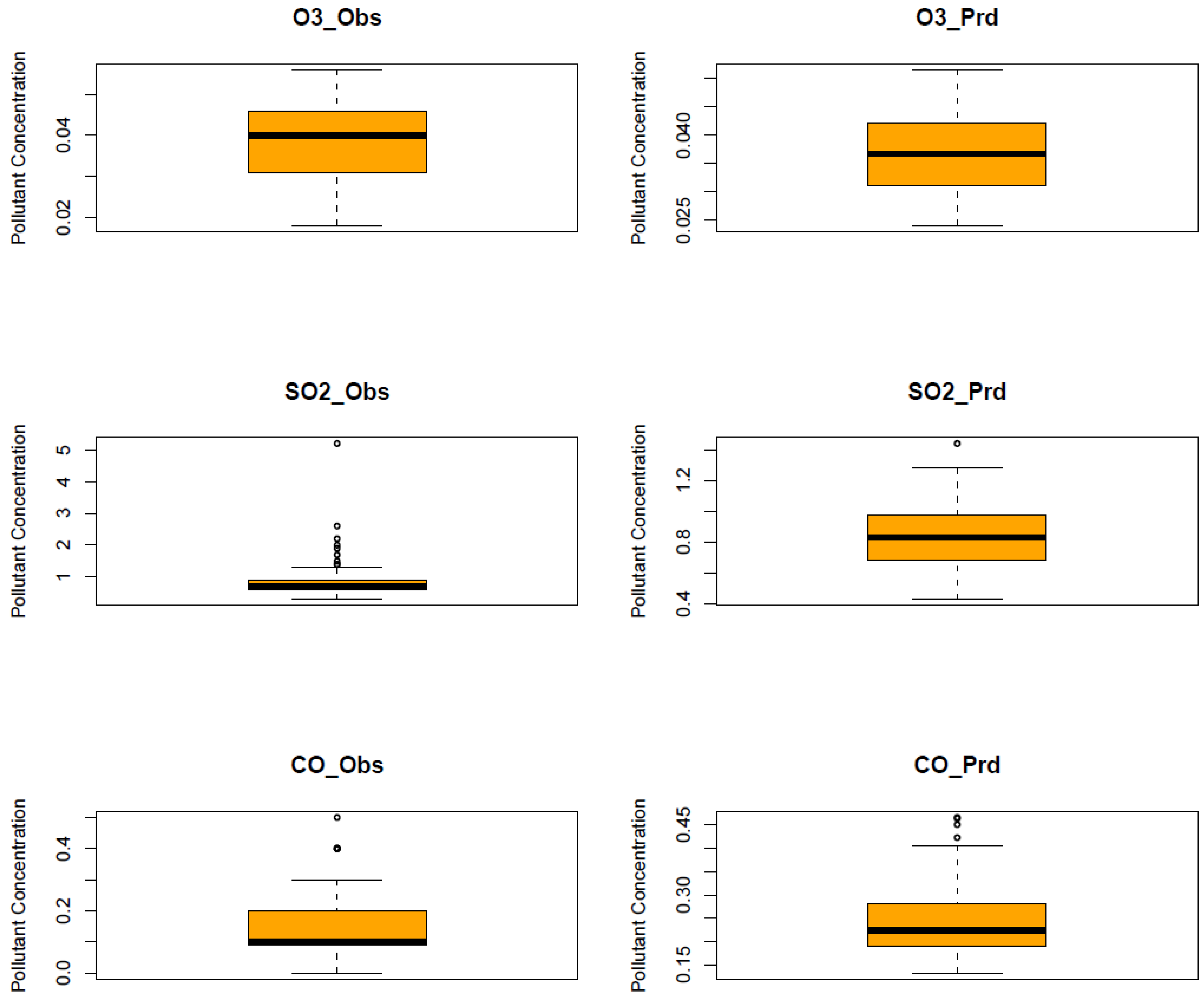
| Item | PM25_Obs (µg/m3) | PM25_Prd (µg/m3) | PM10_Obs (µg/m3) | PM10_Prd (µg/m3) | O3_Obs (ppm) | O3_Prd (ppm) | NO2_Obs (ppb) | NO2_Prd (ppb) | SO2_Obs (ppb) | SO2_Prd (ppb) | CO_Obs (ppm) | CO_Prd (ppm) |
|---|---|---|---|---|---|---|---|---|---|---|---|---|
| Min. | 3.10 | 6.35 | 7.00 | 12.98 | 0.018 | 0.024 | 1.40 | 8.27 | 0.300 | 0.430 | 0.000 | 0.132 |
| 1st Quartile | 6,82 | 8.98 | 14.00 | 17.44 | 0.031 | 0.031 | 5.95 | 12.59 | 0.600 | 0.688 | 0.100 | 0.190 |
| Median | 9.10 | 9.85 | 18.00 | 18.73 | 0.040 | 0.036 | 8.40 | 14.92 | 0.700 | 0.830 | 0.100 | 0.223 |
| Mean | 9.97 | 10.07 | 19.69 | 19.17 | 0.038 | 0.036 | 11.23 | 15.33 | 0.837 | 0.835 | 0.156 | 0.244 |
| 3rd Quartile | 11.50 | 10.87 | 22.0 | 20.60 | 0.046 | 0.042 | 14.00 | 17.60 | 0.900 | 0.971 | 0.200 | 0.278 |
| Max. | 40.70 | 15.85 | 135.0 | 28.85 | 0.056 | 0.051 | 33.00 | 24.33 | 5.200 | 1.439 | 0.500 | 0.466 |
| Item | PM2.5 | PM10 | NO2 | O3 | SO2 | CO |
|---|---|---|---|---|---|---|
| R squared | 0.332 | 0.298 | 0.310 | 0.489 | 0.188 | 0.488 |
| RMSE | 3.01 | 7.55 | 7.56 | 0.008 | 2.18 | 0.008 |
| Item | PM2.5 | PM10 | NO2 | O3 | SO2 | CO |
|---|---|---|---|---|---|---|
| p-value | 0.806 | 0.621 | 2.4 × 10⁻¹² | 1.82 × 10⁻⁵ | 0.971 | 2.2 × 10⁻¹⁶ |
| 95% ci interval | −0.863, 0.677 | −0.634, 2.680 | −5.141, −5.063 | 0.01, 0.003 | −0.102, 0.106 | −0.103, −0.072 |
| Mean difference | −0.095 | 0.523 | −4.102 | 0.002 | 0.001 | −0.087 |
Disclaimer/Publisher’s Note: The statements, opinions and data contained in all publications are solely those of the individual author(s) and contributor(s) and not of MDPI and/or the editor(s). MDPI and/or the editor(s) disclaim responsibility for any injury to people or property resulting from any ideas, methods, instructions or products referred to in the content. |
© 2023 by the authors. Licensee MDPI, Basel, Switzerland. This article is an open access article distributed under the terms and conditions of the Creative Commons Attribution (CC BY) license (https://creativecommons.org/licenses/by/4.0/).
Share and Cite
Tuluri, F.; Remata, R.; Walters, W.L.; Tchounwou, P.B. Impact of Regional Mobility on Air Quality during COVID-19 Lockdown in Mississippi, USA Using Machine Learning. Int. J. Environ. Res. Public Health 2023, 20, 6022. https://doi.org/10.3390/ijerph20116022
Tuluri F, Remata R, Walters WL, Tchounwou PB. Impact of Regional Mobility on Air Quality during COVID-19 Lockdown in Mississippi, USA Using Machine Learning. International Journal of Environmental Research and Public Health. 2023; 20(11):6022. https://doi.org/10.3390/ijerph20116022
Chicago/Turabian StyleTuluri, Francis, Reddy Remata, Wilbur L. Walters, and Paul B. Tchounwou. 2023. "Impact of Regional Mobility on Air Quality during COVID-19 Lockdown in Mississippi, USA Using Machine Learning" International Journal of Environmental Research and Public Health 20, no. 11: 6022. https://doi.org/10.3390/ijerph20116022
APA StyleTuluri, F., Remata, R., Walters, W. L., & Tchounwou, P. B. (2023). Impact of Regional Mobility on Air Quality during COVID-19 Lockdown in Mississippi, USA Using Machine Learning. International Journal of Environmental Research and Public Health, 20(11), 6022. https://doi.org/10.3390/ijerph20116022