Abstract
The purpose of this paper is to develop a multiple dependent state (MDS) sampling plan based on time-truncated sampling schemes for the daily number of cases of the coronavirus disease COVID-19 using gamma distribution under indeterminacy. The proposed sampling scheme parameters include average sample number (ASN) and accept and reject sample numbers when the indeterminacy parameter is known. In addition to the parameters of the proposed sampling schemes, the resultant tables are provided for different known indeterminacy parametric values. The outcomes resulting from various sampling schemes show that the ASN decreases as indeterminacy values increase. This shows that the indeterminacy parameter plays a vital role for the ASN. A comparative study between the proposed sampling schemes and existing sampling schemes based on indeterminacy is also discussed. The projected sampling scheme is illustrated with the help of the daily number of cases of COVID-19 data. From the results and real example, we conclude that the proposed MDS sampling scheme under indeterminacy requires a smaller sample size compared to the single sampling plan (SSP) and the existing MDS sampling plan.
1. Introduction
Nowadays, most of the countries in the world are affected by the current COVID-19 pandemic. COVID-19 is the infectious disease caused by the most recently discovered coronavirus. The most common symptoms of COVID-19 are fever, tiredness, and a dry cough. In more severe cases, the infection can cause pneumonia, severe acute respiratory syndrome, and even death. The number of cases in the pandemic is unknown in most countries worldwide. Aside from that, when cases are spreading, the usual practice of any country is to test the people who show more symptoms; on the other hand, there are some people that do not have any symptoms or only experience a few symptoms [1]. Through these less symptomatic people, the coronavirus spreads more in society. To identify these types of people, more health workers are employing the methodology of randomly testing chosen persons to approximately calculate the actual number of cases in a specified area and, hence, the total state. In such situations, an acceptance sampling plan under indeterminacy is a suitable alternative to testing or assessing the number of cases in a particular locality. Health workers endure pressure to approximate the average daily number of cases of COVID-19 at present and for the next few days, few weeks, or months. For more details, see [2]. The researchers or health workers are interested in testing the null hypothesis that the average daily number of cases is equivalent to the specified average daily number of cases of COVID-19 and the alternative hypothesis that the average daily number of cases of COVID-19 differs significantly. The null hypothesis may be rejected if the average daily number of cases of COVID-19 is more than or equal to the specified average daily number of cases of COVID-19 during the specified number of days.
Numerous authors have studied classical acceptance sampling plans based on time-condensed life tests using various life distributions. A few references to acceptance sampling plans can be seen in [3,4,5,6]. In recent years, different researchers have concentrated on a variety of sampling schemes, from single sampling plans (SSP) to multiple dependent state (MDS) sampling plans based on different distributions. The methodology of the MDS sampling plan was pioneered by [7], and it is based on the attribute assessment procedure, which is based on one out of three situations, namely, acceptance of the lot, rejection of the lot, or the conditional acceptance or rejection of the lot based on the character of future related lots. Subsequently, several authors studied MDS sampling designs on various distributions, such as [8,9,10,11,12,13,14,15,16,17,18].
Two decades ago, the author of [19] introduced a new perception of measurements, namely, neutrosophic logics, the measure of determinacy, and indeterminacy. Subsequently, various researchers discussed neutrosophic logic for a variety of valid problems and proved its effectiveness over fuzzy logic. For additional information, see [20,21,22,23,24,25]. The proposal of neutrosophic statistics was developed based on neutrosophic logic [26,27,28]. The author of [29] stated that neutrosophic statistics provide a lot of information on the measure of determinacy and the measure of indeterminacy. A generalization of traditional statistics is defined as neutrosophic statistics. For more information on acceptance sampling plans using neutrosophic statistics, refer to [30,31,32,33,34]. The authors of [35] proposed a single sampling plan for the inspection of COVID-19 patients using indeterminate Weibull distribution.
The aforementioned sampling designs using traditional statistics and a fuzzy environment do not provide background knowledge about the measure of indeterminacy. Reference [36] studied a single sampling plan based on a fuzzy environment. Reference [37] suggested the outcome of sampling error on assessment based on a fuzzy environment. Some other authors studied the single plan using a fuzzy logic environment; please refer to [38,39,40,41,42].
The present study is based on gamma distribution under indeterminacy. The gamma distribution is a generalization of exponential distribution and is associated with Erlang, normal, chi-square, beta, and some other distributions. This distribution was used for modeling in various life sciences such as epidemiology, computational biology, medical sciences, biostatistics, neuroscience, and so on. In recent years, more researchers studied the applications of gamma distribution in statistical quality control, reliability, queuing theory, survival analysis, and communication engineering. For more details, refer to [43]. The present research is motivated by the idea of neutrosophic statistics given by [26] and extensive studies by Aslam from 2018 onwards on various neutrosophic and indeterminacy probability distributions in different sampling and control chart schemes; some citations are given in the introduction section. Reference [44] originally introduced the indeterminate Weibull distribution and discussed its application in testing wind speed.
Having explored the current research literature related to sampling plans, we were able to conclude that our research work is pioneering, as there has been no previous research work on MDS sampling plan for gamma distribution under indeterminacy. In this paper, we introduce the MDS sampling plan for gamma distribution in the presence of uncertainty. The present piece of work is a targeted MDS sampling plan for gamma distribution under indeterminacy to test the daily number of cases occurring due to COVID-19. It is projected that the developed sampling design will demonstrate a smaller ASN compared with the on-hand sampling designs when testing the daily number of cases occurring due to COVID-19.
In Section 2, we provide a demonstration of the MDS sampling plan for gamma distribution (GD) under indeterminacy. Section 3 examines the comparative study with the existing sampling plans under indeterminacy, as well as existing, classical sampling plans. The proposed sampling plan for the indeterminacy is presented in Section 4 using a real example related to the daily number of cases occurring due to COVID-19. Section 5 deals with the conclusions and future research work.
2. Multiple Dependent State Sampling Plan under Indeterminacy
In this section, the development of the MDS sampling plan is discussed. The following are the essential conditions of pertinence to the proposed MDS sampling plan (see [16]):
- (i)
- The inspection policy consists of taking successive lots manufactured from a continuous manufacturing process. This means that the lots are submitted for inspection serially in the order they have been manufactured in the manufacturing process;
- (ii)
- The submitted lots for the examination have, for all intents and purposes, the same quality level. This means that the manufacturing process has a constant non-conforming fraction;
- (iii)
- The consumer has assurance in the reliability of the manufacturer’s manufacturing process. It means that there is not any basis to consider that any specific lot quality is of inferior quality to the previous lots;
- (iv)
- The quality attribute under contemplation follows a gamma distribution.
The MDS plan is an extension of the SSP. In the MDS plan, the lot-declaring scheme is developed from a one-critical-point to a two-critical-point plan, namely, a lot-accepted critical point and a lot-rejected critical point , which allows the experiential quality level in between () to judge the past, m-lot quality history. Based on this well-versed review, the MDS plan gains an advantage, economically, from governing smaller samples than the SSP.
The following, well-designed methodology for the MDS sampling design was given by [16] under neutrosophic statistics suggested by [44].
Step 1: Select a sample of size n from the batch. These specimens are employed for a life test for a predetermined time . Stipulate the average , and indeterminacy quantity is .
Step 2: The test can be accepted if the average daily number of cases for days is greater or equal to (i.e.,). If the average daily number of cases in days is less than (i.e., > ), then test can be rejected, and the test can be ended where .
Step 3: When , then accept the current lot provided that, in m preceding lots, the mean number of cases is less than or equal to before the test termination time .
The planned MDS sampling plan under indeterminacy is totally differentiated by four values, namely, , and m, where n is the sample size, is the maximum number of allowable items that failed for unconditional acceptance, , is the maximum number of additional items that failed for conditional acceptance , and m is the number of successive lots (previous) needed to make a decision. The attributes’ MDS sampling plan converges to and/or (say), and MDS is an oversimplification of SSP. The operating characteristic (OC) function can reveal the concert of any sampling design.
Applying binomial chance law, the OC function for the MDS sampling design based on GD is expressed as follows [16]:
where
and
where T is a random variable.
Thus, the final expression for the OC function for MDS sampling design is:
The chance of lot approval is obtained at failure probability p under binomial probability distribution.
Suppose that is the neutrosophic random variable that follows the gamma distribution. By following [44], let us assume that is a neutrosophic probability density function (npdf) with the determinate part , indeterminate part , and indeterminacy period . Note that the measure of indeterminacy presents uncertainty in the observations and parameters under an uncertain environment. Remember that considers a neutrosophic random variable (nrv) which abides by the npdf. The npdf is the oversimplification of pdf based on traditional figures. Thus, the planned neutrosophic form of becomes the pdf of traditional figures as soon as = 0. Using this information, the npdf and neutrosophic cumulative distribution function (ncdf) of the GD is determined as under:
and
where is the lower incomplete gamma function, and . is the shape and scale parameters.
The average lifetime of the neutrosophic GD is . A product failure probability before the time is denoted as and is conveyed below:
Here, the neutrosophic termination time is express as product of constant and neutrosophic mean life , i.e., . The scale parameter can be expressed in terms of the neutrosophic mean .
Therefore, Equation (4) can be rewritten in terms of the neutrosophic mean as follows:
where is the ratio of the exact average to the stipulated average.
Suppose that and are the probabilities of type-I and type-II errors. The researcher should pay attention to the projected plan when examining in order to calculate the chance of accepting as soon as the true quantity becomes at least at and the chance of accepting as soon as the false quantity becomes at most at . The plan constants for examining are determined in such a way that the below two inequalities are fulfilled.
where and are defined by
and
Frequently, on-hand sampling schemes are intended to minimize the ASN. Commonly, the foremost intention of any sampling design is to decrease the ASN, which, in turn, minimizes both time and cost for inspection. Correspondingly, the projected MDS sampling design is intended to diminish the ASN for GD for the proposed situation. The non-linear programming method is adopted to get the optimal quantities, and it is expressed as follows:
where and are the failure probabilities of the producer’s and consumer’s risks, respectively. These acceptance chances can be found by means of the following expressions:
and
The proposed plan consists of parameters is obtained by solving the non-linear programming problem in Equation (11) for , , and , and known is placed in Table 1, Table 2, Table 3, Table 4, Table 5, Table 6, Table 7 and Table 8. Table 1 and Table 2 show the GD for , Table 3 and Table 4 show the GD for , Table 5 and Table 6 for , Table 5 and Table 6 for , and Table 7 and Table 8 for . (exponential distribution). From the results in the tables, the following few points can be noticed:

Table 1.
The MDS design values for , , and .
Table 2.
The MDS design values for and .
Table 3.
The MDS design values for and .
Table 4.
The MDS design values for and .
Table 5.
The MDS design values for and .
Table 6.
The MDS design values for , and .
Table 7.
The MDS design values for and .
Table 8.
The MDS design values for and .
- (a)
- The values of the ASN decrease as the value of increases from 0.5 to 1.0;
- (b)
- The ASN decreases as the shape parameter increases from when other parameters are fixed;
- (c)
- In addition, to minimize ASN values, the indeterminacy parameter . shows a significant influence;
- (d)
- The ASN is larger for the traditional MDS plan than the proposed MDS sampling plan under indeterminacy;
- (e)
- (f)
- Furthermore, it is depicted by the OC curves that the proposed MDS sampling plan under indeterminacy is more efficient than the existing single sampling plan.
3. Comparative Studies
This section deals with a comparative study of the proposed sampling scheme with the existing SSP. The efficiency of the developed sampling plan is calculated based on the ASN; a low-sample-size design is more economical to test the hypothesis about the mean. It is important to note that the proposed MDS sampling plan under indeterminacy is the generalization of the MDS sampling plan for traditional statistics if no uncertainty or indeterminacy happens when measuring the average. If = 0, the proposed MDS sampling plan under indeterminacy becomes the MDS sampling plan in hand. In Table 1, Table 2, Table 3, Table 4, Table 5, Table 6, Table 7 andTable 8, the first column, i.e., at = 0, is the plan parameter of the traditional or existing MDS sampling plan. From the results, we conclude that the ASN is large in the traditional MDS sampling plan compared with the proposed MDS sampling plan. For example, when = 1.4, = 2, and = 0.5, from Table 1 it can be seen that = 39 from the plan under classical statistics, and = 34 for the projected sampling plan when = 0.05. Furthermore, when = 1, the GD becomes an exponential distribution; we constructed Table 7 and Table 8 for exponential distribution for comparison purposes. Table 7 depicts that the GD shows a lower sample number compared with exponential distribution. For example, when = 1.5, = 0.5, and = 0.04, Table 7 shows that the ASN is 42, whereas the proposed plan values are ASN = 25 for = 2, ASN = 24 for = 2.5, and ASN = 20 for = 3. From this study, it is concluded that the projected plan under indeterminacy is more efficient than the existing sampling plan under traditional statistics with respect to sample size. The operating characteristic (OC) curve of the plan of the GD when and is depicted in Figure 1 and Figure 2. Therefore, the application of the proposed plan for testing the null hypothesis demands a smaller sample compared to the on-hand plan. The OC curve in Figure 1 also shows the same performance. Researchers can apply the proposed plan under uncertainty to save time and money.
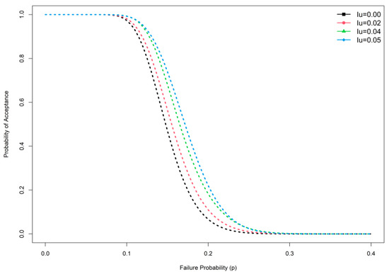
Figure 1.
OC curve plan at different indeterminacy values.
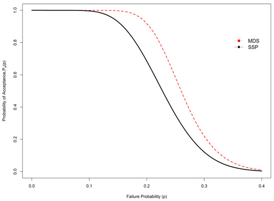
Figure 2.
OC curve comparison between SSP and MDS under indeterminacy.
4. Applications for COVID-19 Data
The practical utility of the anticipated sampling design for the GD under indeterminacy is presented in this section using a real example. The real data set is constituted of newly notified cases on a daily basis. These data consist of a 61-day COVID-19 data set taken from Italy, which reports the daily number of cases between 13 June and 12 August 2021. For more details, refer to the new, discrete distribution with application to COVID-19 data developed by [45]. For ready reference, the data are reported here:
Daily number of cases: 52, 26, 36, 63, 52, 37, 35, 28, 17, 21, 31, 30, 10, 56, 40, 14, 28, 42, 24, 21, 28, 22, 12, 31, 24, 14, 13, 25, 12, 7, 13, 20, 23, 9, 11, 13, 3, 7, 10, 21, 15, 17, 5, 7, 22, 24, 15, 19, 18, 16, 5, 20, 27, 21, 27, 24, 22, 11, 22, 31, and 31.
The daily number of cases occurring due to COVID-19 plays a vital role for medical administrators in every nation in the world nowadays. COVID-19 cases encounter unpredictability and uncertainty; thus, the daily number of cases data become a probability distribution under neutrosophic information. The government administrators are anxious to monitor the average daily number of cases under indeterminacy.
It is established that the daily number of cases data can be drawn from the GD with shape parameter = 3.1946 and scale parameter , and the maximum distance between the real-time data and the fitted of GD can be found from the Kolmogorov–Smirnov test statistic 0.0803 and also the p-value 0.8262. The demonstration of the goodness of fit for the given model, the empirical and theoretical pdfs, cdf, P-P plot and Q-Q plots for the GD for the daily number of cases data are shown in Figure 3. Therefore, GD is well fitted for the daily number of cases of COVID-19 data. The plan parameters for this shape parameter are shown in Table 9 and Table 10. For the proposed plan, the shape parameter is when = 0.04. Suppose that medical administrators are concerned with testing with the aid of the proposed sampling plan when = 0.04,, = 1.4, = 0.5, and = 0.10. From Table 9, it can be noted that = 55, , = 14, m = 1, and ASN = 55. The developed MDS sampling plan works by accepting the null hypothesis if the average daily number of cases in 6 days is more than equal to daily number of cases. A sample of 55 daily due to COVID-19 can be selected at random for a crowd of people, and the null hypothesis . If the average daily number of cases before is less than or equal to 6 days, then the crowd of people can be accepted, and the crowd of people can be rejected if it is greater than 14 days. If the prevalence of the number of cases of COVID-19 is between 6 and 14 days, a property of the present crowd of people can be deferred until the preceding crowd of people has be tested. From the data, it can be noted that an average daily number of cases of COVID-19 was greater than equal to encounter in more than 36 days; therefore, the claim about the average daily number of cases could be rejected. Hence, medical administrators could suggest to the government that the average daily number of cases of COVID-19 was at an unendurable stage. Therefore, the proposed sampling plan is useful in medical applications, specifically, in taking decisions regarding the daily number of cases of COVID-19 and the average daily number of COVID-19 patients, and this is very important for any government making policy decisions.
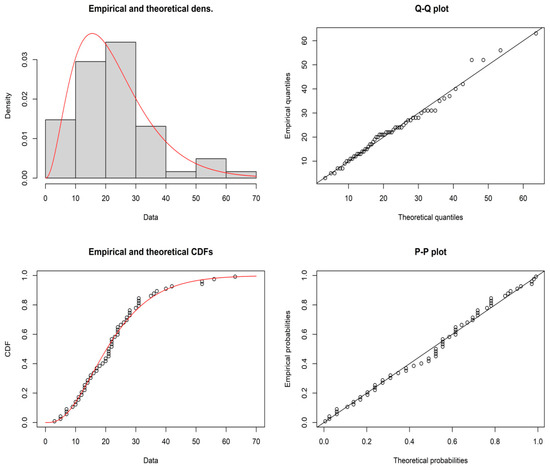
Figure 3.
Pictorial presentation of various plots for the GD for daily number of cases data.
Table 9.
The MDS design values for and .
Table 10.
The MDS design values for and .
5. Conclusions
A broad analysis of the daily number of cases of COVID-19 for gamma distribution based on indeterminacy situation for a time-truncated MDS sampling design was formulated. The sampling plan’s quantities were determined at pre-assigned values of indeterminacy parameters. Comprehensive tables were given for ready reference to the researchers for the known indeterminacy constant values. The formulated MDS sampling design based on indeterminacy was compared with the already available sampling schemes based on classical statistics. The results showed that the formulated MDS sampling plan under indeterminacy was more reasonable than the already available SSP under indeterminacy and traditional MDS sampling plans. In addition, the developed MDS under indeterminacy was greatly cheaper to run than the SSP. It is important to note that the indeterminacy parameter showed a prime role in decreasing ASN values, which means that, if the indeterminacy value increased then the ASN values were in decreasing trend. Therefore, the formulated MDS sampling plan under indeterminacy is more useful to scientists, in particular to medical practitioners and those who are studying or testing sensitive issues which require skilled researchers and need more money. Thus, the formulated MDS sampling plan under indeterminacy is approved to be applicable for testing the average daily number of cases of COVID-19. The exemplification based on the daily number of cases of COVID-19 data for the formulated MDS sampling plan under indeterminacy showed confirmation. The formulated MDS sampling plan under indeterminacy can be used by other researchers working in various fields. Considering a control chart methodology based on multiple dependent state sampling plans will be the topic of a further research study to monitor the mean.
Author Contributions
Conceptualization, M.A. (Muhammad Aslam) and G.S.R.; methodology, M.A. (Muhammad Aslam) and M.A. (Mohammed Albassam); software, G.S.R.; validation, M.A. (Muhammad Aslam) and M.A. (Mohammed Albassam); formal analysis, M.A. (Mohammed Albassam); investigation, M.A. (Muhammad Aslam); resources, G.S.R.; data curation, M.A. (Mohammed Albassam); writing—original draft preparation, M.A. (Muhammad Aslam), G.S.R. and M.A. (Mohammed Albassam); writing—review and editing, M.A. (Muhammad Aslam), G.S.R. and M.A. (Mohammed Albassam); visualization, G.S.R.; supervision, M.A. (Muhammad Aslam); project administration, M.A. (Muhammad Aslam); funding acquisition, M.A. (Muhammad Aslam). All authors have read and agreed to the published version of the manuscript.
Funding
This research received no external funding.
Institutional Review Board Statement
Not applicable.
Informed Consent Statement
Not applicable.
Data Availability Statement
Not applicable.
Acknowledgments
The authors are deeply thankful to the editor and reviewers for their valuable suggestions to improve the quality and presentation of the paper. The work was supported by the Deanship of Scientific Research (DSR) at King Abdulaziz University. The authors, therefore, thank the DSR for their financial and technical support.
Conflicts of Interest
The authors declare no conflict of interest.
Abbreviations
| MDS | Multiple dependent state |
| ASN | Average sample number |
| SSP | Single sampling plan |
| COVID-19 | Coronavirus disease |
| OC | Operating characteristic |
| GD | Gamma distribution |
References
- Mizumoto, K.; Kagaya, K.; Zarebski, A.; Chowell, G. Estimating the asymptomatic proportion of coronavirus disease 2019 (COVID-19) cases on board the Diamond Princess cruise ship, Yokohama, Japan, 2020. Euro Surveill. Bull. Eur. Sur Mal. Transm. Eur. Commun. Dis. Bull. 2020, 25, 2000180. [Google Scholar] [CrossRef] [Green Version]
- Hogan, C.A.; Sahoo, M.K.; Pinsky, B.A. Sample pooling as a strategy to detect community transmission of SARS-CoV-2. J. Am. Med. Assoc. 2020, 323, 1967–1969. [Google Scholar] [CrossRef] [Green Version]
- Kantam, R.R.L.; Rosaiah, K.; Rao, G.S. Acceptance sampling based on life tests: Log-logistic model. J. Appl. Stat. 2001, 28, 121–128. [Google Scholar] [CrossRef]
- Tsai, T.-R.; Wu, S.-J. Acceptance sampling based on truncated life tests for generalized Rayleigh distribution. J. Appl. Stat. 2006, 33, 595–600. [Google Scholar] [CrossRef]
- Yan, A.; Liu, S.; Dong, X. Variables two stage sampling plans based on the coefficient of variation. J. Adv. Mech. Des. Syst. Manuf. 2016, 10, JAMDSM0002. [Google Scholar] [CrossRef] [Green Version]
- Yen, C.-H.; Lee, C.-C.; Lo, K.-H.; Shiue, Y.-R.; Li, S.-H. A Rectifying Acceptance Sampling Plan Based on the Process Capability Index. Mathematics 2020, 8, 141. [Google Scholar] [CrossRef] [Green Version]
- Wortham, A.W.; Baker, R.C. Multiple deferred state sampling inspection. Int. J. Prod. Res. 1976, 14, 719–731. [Google Scholar] [CrossRef]
- Soundararajan, V.; Vijayaraghavan, R. Construction and selection of multiple dependent (deferred) state sampling plan. J. Appl. Stat. 1990, 17, 397–409. [Google Scholar] [CrossRef]
- Govindaraju, K.; Subramani, K. Selection of multiple deferred (dependent) state sampling plans for given acceptable quality level and limiting quality level. J. Appl. Stat. 1993, 20, 423–428. [Google Scholar] [CrossRef]
- Balamurali, S.; Jun, C.H. Multiple dependent state sampling plans for lot acceptance based on measurement data. Eur. J. Oper. Res. 2007, 180, 1221–1230. [Google Scholar] [CrossRef]
- Subramani, K.; Haridoss, V. Development of multiple deferred state sampling plan based on minimum risks using the weighted poisson distribution for given acceptance quality level and limiting quality level. Int. J. Qual. Eng. Technol. 2012, 3, 168–180. [Google Scholar] [CrossRef]
- Aslam, M.; Azam, M.; Jun, C. Multiple dependent state sampling plan based on process capability index. J. Test. Eval. 2013, 41, 340–346. [Google Scholar] [CrossRef]
- Subramani, K.; Haridoss, V. Selection of multiple deferred state MDS-1 sampling plan for given acceptable quality level and limiting quality level involving minimum risks using weighted Poisson distribution. Int. J. Qual. Res. 2013, 7, 347–358. [Google Scholar]
- Aslam, M.; Yen, C.H.; Chang, C.H.; Jun, C.H. Multiple dependent state variable sampling plans with process loss consideration. Int. J. Adv. Manuf. 2014, 71, 1337–1343. [Google Scholar] [CrossRef]
- Yan, A.; Liu, S.; Dong, X. Designing a multiple dependent state sampling plan based on the coefficient of variation. Springerplus 2016, 5, 1447. [Google Scholar] [CrossRef] [Green Version]
- Balamurali, S.; Jeyadurga, P.; Usha, M. Designing of multiple deferred state sampling plan for generalized inverted exponential distribution. Seq. Anal. 2017, 36, 76–86. [Google Scholar] [CrossRef]
- Wang, T.-C.; Wu, C.-W.; Shu, M.-H. A variables-type multiple-dependent-state sampling plan based on the lifetime performance index under a Weibull distribution. Ann. Oper. Res. 2022, 311, 381–399. [Google Scholar] [CrossRef]
- Rao, G.S.; Rosaiah, K.; RameshNaidu, C. Design of multiple-deferred state sampling plans for exponentiated half logistic distribution. Cogent Math. Stat. 2020, 7, 1857915. [Google Scholar]
- Smarandache, F. Neutrosophy. Neutrosophic Probability, Set, and Logic, ProQuest Information & Learning. Ann. Arbor Mich. USA 1998, 105, 118–123. [Google Scholar]
- Smarandache, F.; Khalid, H.E. Neutrosophic Precalculus and Neutrosophic Calculus: Infinite Study; Pons Publishing House: Brussels, Belgium, 2015. [Google Scholar]
- Peng, X.; Dai, J. Approaches to single-valued neutrosophic MADM based on MABAC, TOPSIS and new similarity measure with score function. Neural. Comput. Appl. 2018, 29, 939–954. [Google Scholar] [CrossRef]
- Abdel-Basset, M.; Mohamed, M.; Elhoseny, M.; Chiclana, F.; Zaied, A.E.-N.H. Cosine similarity measures of bipolar neutrosophic set for diagnosis of bipolar disorder diseases. Artif. Intell. Med. 2019, 101, 101735. [Google Scholar] [CrossRef]
- Nabeeh, N.A.; Smarandache, F.; Abdel-Basset, M.; El-Ghareeb, H.A.; Aboelfetouh, A. An integrated neutrosophic-topsis approach and its application to personnel selection: A new trend in brain processing and analysis. IEEE Access 2019, 7, 29734–29744. [Google Scholar] [CrossRef]
- Pratihar, J.; Kumar, R.; Dey, A.; Broumi, S. Transportation Problem in Neutrosophic Environment Neutrosophic Graph Theory and Algorithms; IGI Global: Hershey, PA, USA, 2020; pp. 180–212. [Google Scholar]
- Pratihar, J.; Kumar, R.; Edalatpanah, S.; Dey, A. Modified Vogel’s approximation method for transportation problem under uncertain environment. Complex Intell. Syst. 2021, 7, 29–40. [Google Scholar] [CrossRef]
- Smarandache, F. Introduction to Neutrosophic Statistics: Infinite Study; Sitech & Education Publishing: Craiova, Romania, 2014. [Google Scholar]
- Chen, J.; Ye, J.; Du, S. Scale effect and anisotropy analyzed for neutrosophic numbers of rock joint roughness coefficient based on neutrosophic statistics. Symmetry 2017, 9, 208. [Google Scholar] [CrossRef]
- Chen, J.; Ye, J.; Du, S.; Yong, R. Expressions of rock joint roughness coefficient using neutrosophic interval statistical numbers. Symmetry 2017, 9, 123. [Google Scholar] [CrossRef]
- Aslam, M. Introducing Kolmogorov–Smirnov Tests under Uncertainty: An Application to Radioactive Data. ACS Omega 2019, 5, 914–917. [Google Scholar] [CrossRef] [Green Version]
- Aslam, M. A new sampling plan using neutrosophic process loss consideration. Symmetry 2018, 10, 132. [Google Scholar] [CrossRef] [Green Version]
- Aslam, M. Design of Sampling Plan for exponential distribution under neutrosophic statistical interval method. IEEE Access 2018, 6, 64153–64158. [Google Scholar] [CrossRef]
- Aslam, M. A new attribute sampling plan using neutrosophic statistical interval method. Complex Intell. Syst. 2019, 5, 365–370. [Google Scholar] [CrossRef] [Green Version]
- Aslam, M.; Jeyadurga, P.; Balamurali, S.; AL-Marshadi, A.H. Time-truncated group plan under a Weibull distribution based on neutrosophic statistics. Mathematics 2019, 7, 905. [Google Scholar] [CrossRef] [Green Version]
- Alhasan, K.F.H.; Smarandache, F. Neutrosophic Weibull distribution and neutrosophic family Weibull distribution: Infinite Study. Neutrosophic Sets Syst. 2019, 28, 191–199. [Google Scholar]
- Rao, G.S.; Aslam, M. Inspection plan for COVID-19 patients for Weibull distribution using repetitive sampling under indeterminacy. BMC Med. Res. Methodol. 2021, 21, 229. [Google Scholar] [CrossRef] [PubMed]
- Jamkhaneh, E.B.; Sadeghpour-Gildeh, B.; Yari, G. Important criteria of rectifying inspection for single sampling plan with fuzzy parameter. Int. J. Contemp. Math. Sci. 2009, 4, 1791–1801. [Google Scholar]
- Jamkhaneh, E.B.; Sadeghpour-Gildeh, B.; Yari, G. Inspection error and its effects on single sampling plans with fuzzy parameters. Struct. Multidiscip. Optim. 2011, 43, 555–560. [Google Scholar] [CrossRef]
- Sadeghpour Gildeh, B.; Baloui Jamkhaneh, E.; Yari, G. Acceptance single sampling plan with fuzzy parameter. Iran. J. Fuzzy Syst. 2011, 8, 47–55. [Google Scholar]
- Afshari, R.; Sadeghpour Gildeh, B. Designing a multiple deferred state attribute sampling plan in a fuzzy environment. Am. J. Math. Manag. Sci. 2017, 36, 328–345. [Google Scholar] [CrossRef]
- Tong, X.; Wang, Z. Fuzzy acceptance sampling plans for inspection of geospatial data with ambiguity in quality characteristics. Comput. Geosci. 2012, 48, 256–266. [Google Scholar] [CrossRef]
- Uma, G.; Ramya, K. Impact of Fuzzy Logic on Acceptance Sampling Plans—A Review. Autom. Auton. Syst. 2015, 7, 181–185. [Google Scholar]
- Shawky, A.I.; Aslam, M.; Khan, K. Multiple dependent state sampling-based chart using belief statistic under neutrosophic statistics. J. Math. 2020, 2020, 7680286. [Google Scholar] [CrossRef]
- Okagbue, H.; Adamu, M.O.; Anake, T.A. Approximations for the inverse cumulative distribution function of the gamma distribution used in wireless communication. Heliyon 2020, 6, e05523. [Google Scholar] [CrossRef]
- Aslam, M. Testing average wind speed using sampling plan for Weibull distribution under indeterminacy. Sci. Rep. 2021, 11, 7532. [Google Scholar] [CrossRef] [PubMed]
- Almetwally, E.M.; Abdo, D.A.; Hafez, E.H.; Jawa, T.M.; Sayed-Ahmed, N.; Almongy, H.M. The new discrete distribution with application to COVID-19 Data. Results Phys. 2022, 32, 104987. [Google Scholar] [CrossRef] [PubMed]
Publisher’s Note: MDPI stays neutral with regard to jurisdictional claims in published maps and institutional affiliations. |
© 2022 by the authors. Licensee MDPI, Basel, Switzerland. This article is an open access article distributed under the terms and conditions of the Creative Commons Attribution (CC BY) license (https://creativecommons.org/licenses/by/4.0/).