
Socioeconomic Disparities in Hypertension by Levels of Green Space Availability: A Cross-Sectional Study in Philadelphia, PA


Abstract
:1. Introduction
2. Materials and Methods
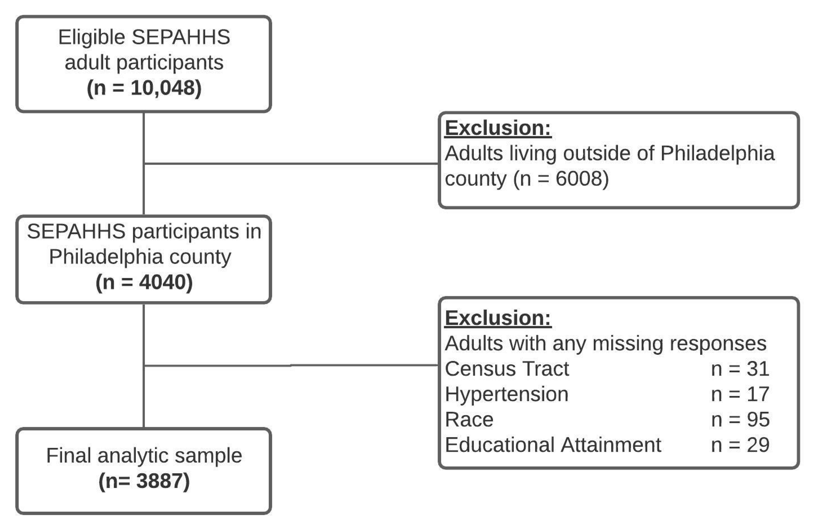
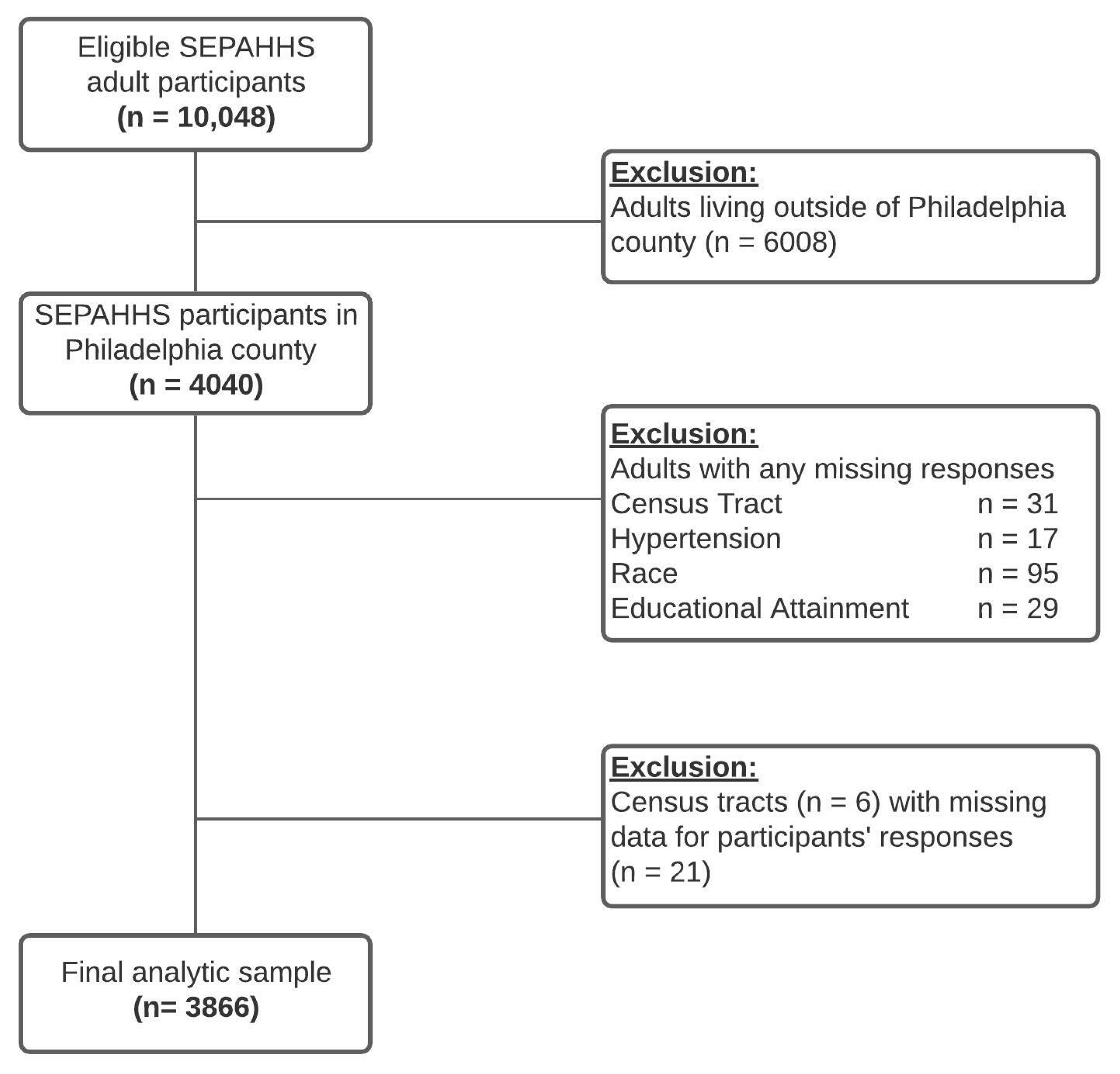
2.1. Study Setting
2.2. Outcome (Hypertension)
2.3. Exposure
2.4. Effect Modifier (Green Spaces)
2.5. Covariates
2.6. Statistical Data Analysis
3. Results
4. Discussion
5. Conclusions
Author Contributions
Funding
Institutional Review Board Statement
Informed Consent Statement
Data Availability Statement
Acknowledgments
Conflicts of Interest
Appendix A

| Measure | Categorization |
|---|---|
| Median household income | Q1 (USD 11,473 to 27,188) Q2 (USD 27,202 to 39,225) Q3 (USD 39,318 to 53,708) Q4 (USD 53,742 to 145,104) |
| Tree canopy cover | Low (2–11.8%) Medium (11.8–20.9%) High (21.4–87.9%) |
| Distance to nearest park 1 | Low (0–175.6 m) Medium (176.8–332.4 m) High (332.4–2222 m) |
| Normalized Difference Vegetation Index (NDVI) | Low (−0.075 to 0.142) Medium (0.142 to 0.237) High (0.238 to 0.530) |
| Inclusion | Exclusion |
|---|---|
| Community Parks, Farms, Gardens, Greenhouses, Nursery, Linear Parks, Parkways, Metropolitan Parks, Mini Parks, Neighborhood Parks, Regional/Watershed Parks, Square/Plaza Parks, and Watershed/Conservation Parks. | Athletic Fields, Barns, Batting Cages, Boathouses, Concessions/Retail/Cafes, Dugouts, Environmental Education Centers, Garages/Maintenance/Storage, Golf Courses and Ranges, Greenhouses/Nursery, Guard Boxes, Historic Houses, Ice Rinks, Lot/Breezeway/Island, Multi-Use Area, Multi-Use Building, Museums, Older Adult Centers, Pavilion/Shelter, Pool, Pumping Station, Recreation Building, Recreation Center, Recreation Site, Restrooms, Shed, Stables, Stage/Stands, Statue/Monument/Sculpture, Weigh Station, Youth and Tot/Play Areas, and Zoo Habitat. |
| OR (95% CI) | p-Value | |
|---|---|---|
| Median Household Income | ||
| Q1 | 1.00 (Ref.) | |
| Q2 | 0.78 (0.58; 1.06) | 0.118 |
| Q3 | 0.73 (0.53; 1.02) | 0.064 |
| Q4 | 0.51 (0.36; 0.72) | <0.001 * |
| Age (years) | ||
| 18–34 | 1.00 (Ref.) | |
| 35–49 | 3.13 (2.04; 4.79) | <0.001 * |
| 50–64 | 11.26 (7.78; 16.28) | <0.001 * |
| 65+ | 22.28 (15.18; 32.71) | <0.001 * |
| Sex | ||
| Male | 1.00 (Ref.) | |
| Female | 0.94 (0.76; 1.16) | 0.565 |
| Race/Ethnicity | ||
| NH White 1 | 1.00 (Ref.) | |
| NH Black 1 | 2.13 (1.64; 2.76) | <0.001 * |
| Hispanic/Latino | 1.23 (0.8; 1.89) | 0.348 |
| Other | 0.75 (0.47; 1.21) | 0.238 |
| Our Study | Philadelphia * | |
|---|---|---|
| Hypertension (yes) | 38.3% | 38.2% |
| Age (years) | ||
| 18–34 | 30.2% | 32.4% |
| 35–49 | 17.9% | 29.8% |
| 50–64 | 32.7% | 21.8% |
| 65+ | 19.1% | 16.0% |
| Sex | ||
| Male | 45.0% | 46.5% |
| Female | 55.0% | 53.5% |
| Race/Ethnicity | ||
| NH White | 39.9% | 38.2% |
| NH Black | 41.4% | 41.5% |
| Hispanic/Latino | 12.0% | 12.6% |
| Other | 6.8% | 7.7% |

References
- US EPA. REG 01. “What Is Open Space/Green Space? | Urban Environmental Program in New England”. Overviews & Factsheets. Available online: https://www3.epa.gov/region1/eco/uep/openspace.html (accessed on 12 January 2022).
- Twohig-Bennett, C.; Jones, A. The health benefits of the great outdoors: A systematic review and meta-analysis of greenspace exposure and health outcomes. Environ. Res. 2018, 166, 628–637. [Google Scholar] [CrossRef]
- Maas, J.; Verheij, R.A.; de Vries, S.; Spreeuwenberg, P.; Schellevis, F.G.; Groenewegen, P.P. Morbidity is related to a green living environment. J. Epidemiol. Community Health 2009, 63, 967–973. [Google Scholar] [CrossRef] [Green Version]
- Wolch, J.R.; Byrne, J.; Newell, J.P. Urban green space, public health, and environmental justice: The challenge of making cities ‘just green enough’. Landsc. Urban Plan. 2014, 125, 234–244. [Google Scholar] [CrossRef] [Green Version]
- Department of Economic and Social Affairs; United Nations. World Urbanization Prospects: The 2018 Revision (ST/ESA/SER.A/420). United Nations, New York. 2019. Available online: https://population.un.org/wup/Publications/Files/WUP2018-Report.pdf (accessed on 12 January 2022).
- Ali, M.U.; Liu, G.; Yousaf, B.; Ullah, H.; Abbas, Q.; Munir, M.A.M. A systematic review on global pollution status of particulate matter-associated potential toxic elements and health perspectives in urban environment. Environ. Geochem. Heal. 2018, 41, 1131–1162. [Google Scholar] [CrossRef]
- Frumkin, H. Urban sprawl and public health. Public Health Rep. 2002, 117, 201–217. [Google Scholar] [CrossRef]
- US EPA. Green Streets and Community Open Space. 11 January 2018. Available online: https://www.epa.gov/G3/green-streets-and-community-open-space (accessed on 12 January 2022).
- Kondo, M.C.; Fluehr, J.M.; McKeon, T.P.; Branas, C.C. Urban Green Space and Its Impact on Human Health. Int. J. Environ. Res. Public Heal. 2018, 15, 445. [Google Scholar] [CrossRef] [Green Version]
- Richardson, E.A.; Mitchell, R.; Hartig, T.; de Vries, S.; Astell-Burt, T.; Frumkin, H. Green cities and health: A question of scale? J. Epidemiol. Community Health 2012, 66, 160–165. [Google Scholar] [CrossRef] [Green Version]
- Taylor, L.; Hochuli, D.F. Defining greenspace: Multiple uses across multiple disciplines. Landsc. Urban Plan. 2017, 158, 25–38. [Google Scholar] [CrossRef] [Green Version]
- Astell-Burt, T.; Feng, X. Urban green space, tree canopy and prevention of cardiometabolic diseases: A multilevel longitudinal study of 46 786 Australians. Int. J. Epidemiol. 2020, 49, 926–933. [Google Scholar] [CrossRef] [Green Version]
- Wheeler, B.W.; Lovell, R.; Higgins, S.L.; White, M.P.; Alcock, I.; Osborne, N.J.; Husk, K.; Sabel, C.E.; Depledge, M.H. Beyond greenspace: An ecological study of population general health and indicators of natural environment type and quality. Int. J. Health Geogr. 2015, 14, 17. [Google Scholar] [CrossRef] [Green Version]
- Aram, F.; Garcia, E.H.; Solgi, E.; Mansournia, S. Urban green space cooling effect in cities. Heliyon 2019, 5, e01339. [Google Scholar] [CrossRef] [Green Version]
- Nowak, D.J.; Crane, D.E.; Stevens, J.C. Air pollution removal by urban trees and shrubs in the United States. Urban For. Urban Green. 2006, 4, 115–123. [Google Scholar] [CrossRef]
- Liu, W.; Chen, W.; Peng, C. Assessing the effectiveness of green infrastructures on urban flooding reduction: A community scale study. Ecol. Model. 2014, 291, 6–14. [Google Scholar] [CrossRef]
- Brown, S.C.; Perrino, T.; Lombard, J.; Wang, K.; Toro, M.; Rundek, T.; Gutierrez, C.M.; Dong, C.; Plater-Zyberk, E.; Nardi, M.I.; et al. Health Disparities in the Relationship of Neighborhood Greenness to Mental Health Outcomes in 249,405 U.S. Medicare Beneficiaries. Int. J. Environ. Res. Public Health 2018, 15, 430. [Google Scholar] [CrossRef] [PubMed] [Green Version]
- Lachowycz, K.; Jones, A.P. Greenspace and obesity: A systematic review of the evidence. Obes. Rev. 2011, 12, e183–e189. [Google Scholar] [CrossRef]
- Akpinar, A. How is quality of urban green spaces associated with physical activity and health? Urban For. Urban Green. 2016, 16, 76–83. [Google Scholar] [CrossRef]
- Richardson, E.; Pearce, J.; Mitchell, R.; Kingham, S. Role of physical activity in the relationship between urban green space and health. Public Health 2013, 127, 318–324. [Google Scholar] [CrossRef] [Green Version]
- Jennings, V.; Bamkole, O. The Relationship between Social Cohesion and Urban Green Space: An Avenue for Health Promotion. Int. J. Environ. Res. Public Health 2019, 16, 452. [Google Scholar] [CrossRef] [Green Version]
- Brunner, E. Socioeconomic determinants of health: Stress and the biology of inequality. BMJ 1997, 314, 1472. [Google Scholar] [CrossRef]
- Lee, J.; Tsunetsugu, Y.; Takayama, N.; Park, B.-J.; Li, Q.; Song, C.; Komatsu, M.; Ikei, H.; Tyrväinen, L.; Kagawa, T.; et al. Influence of Forest Therapy on Cardiovascular Relaxation in Young Adults. Evid. Based Complementary Altern. Med. 2014, 2014, 1–7. [Google Scholar] [CrossRef]
- Mobley, L.R.; Root, E.; Finkelstein, E.A.; Khavjou, O.; Farris, R.P.; Will, J.C. Environment, Obesity, and Cardiovascular Disease Risk in Low-Income Women. Am. J. Prev. Med. 2006, 30, 327–332.e1. [Google Scholar] [CrossRef] [PubMed]
- Dzhambov, A.M.; Markevych, I.; Lercher, P. Greenspace seems protective of both high and low blood pressure among residents of an Alpine valley. Environ. Int. 2018, 121, 443–452. [Google Scholar] [CrossRef] [PubMed]
- Browning, M.H.; Rigolon, A.; McAnirlin, O.; McAnirlin, O. Where greenspace matters most: A systematic review of urbanicity, greenspace, and physical health. Landsc. Urban Plan. 2021, 217, 104233. [Google Scholar] [CrossRef]
- Zhang, L.; Tan, P.Y. Associations between Urban Green Spaces and Health are Dependent on the Analytical Scale and How Urban Green Spaces are Measured. Int. J. Environ. Res. Public Health 2019, 16, 578. [Google Scholar] [CrossRef] [Green Version]
- Knobel, P.; Kondo, M.; Maneja, R.; Zhao, Y.; Dadvand, P.; Schinasi, L.H. Associations of objective and perceived greenness measures with cardiovascular risk factors in Philadelphia, PA: A spatial analysis. Environ. Res. 2021, 197, 110990. [Google Scholar] [CrossRef]
- Mitchell, R.; Popham, F. Effect of exposure to natural environment on health inequalities: An observational population study. Lancet 2008, 372, 1655–1660. [Google Scholar] [CrossRef] [Green Version]
- Tamosiunas, A.; Grazuleviciene, R.; Luksiene, D.; Dedele, A.; Reklaitiene, R.; Baceviciene, M.; Vencloviene, J.; Bernotiene, G.; Radisauskas, R.; Malinauskiene, V.; et al. Accessibility and use of urban green spaces, and cardiovascular health: Findings from a Kaunas cohort study. Environ. Health 2014, 13, 20. [Google Scholar] [CrossRef] [Green Version]
- Wilker, E.H.; Wu, C.-D.; McNeely, E.; Mostofsky, E.; Spengler, J.; Wellenius, G.A.; Mittleman, M.A. Green space and mortality following ischemic stroke. Environ. Res. 2014, 133, 42–48. [Google Scholar] [CrossRef] [Green Version]
- Liburd, L.C.; Hall, J.E.; Mpofu, J.J.; Williams, S.M.; Bouye, K.; Penman-Aguilar, A. Addressing Health Equity in Public Health Practice: Frameworks, Promising Strategies, and Measurement Considerations. Annu. Rev. Public Health 2020, 41, 417–432. [Google Scholar] [CrossRef] [Green Version]
- Krieger, N.; Williams, D.R.; Moss, N.E. Measuring Social Class in US Public Health Research: Concepts, Methodologies, and Guidelines. Annu. Rev. Public Health 1997, 18, 341–378. [Google Scholar] [CrossRef] [Green Version]
- Loucks, E.B.; Abrahamowicz, M.; Xiao, Y.; Lynch, J.W. Associations of education with 30 year life course blood pressure trajectories: Framingham Offspring Study. BMC Public Health 2011, 11, 139. [Google Scholar] [CrossRef] [PubMed] [Green Version]
- Camacho, P.A.; Gomez-Arbelaez, D.; Molina, D.I.; Sanchez, G.; Arcos, E.; Narvaez, C.; García, H.; Pérez, M.; Hernandez, E.A.; Duran, M.; et al. Social disparities explain differences in hypertension prevalence, detection and control in Colombia. J. Hypertens. 2016, 34, 2344–2352. [Google Scholar] [CrossRef] [PubMed]
- Rosengren, A.; Subramanian, S.V.; Islam, S.; Chow, C.K.; Avezum, A.; Kazmi, K.; Sliwa, K.; Zubaid, M.; Rangarajan, S.; Yusuf, S.; et al. Education and risk for acute myocardial infarction in 52 high, middle and low-income countries: INTERHEART case-control study. Heart 2009, 95, 2014–2022. [Google Scholar] [CrossRef] [PubMed]
- Rosengren, A.; Smyth, A.; Rangarajan, S.; Ramasundarahettige, C.; Bangdiwala, S.I.; Alhabib, K.F.; Avezum, A.; Boström, K.B.; Chifamba, J.; Gulec, S.; et al. Socioeconomic status and risk of cardiovascular disease in 20 low-income, middle-income, and high-income countries: The Prospective Urban Rural Epidemiologic (PURE) study. Lancet Glob. Health 2019, 7, e748–e760. [Google Scholar] [CrossRef] [Green Version]
- Gullón, P.; Díez, J.; Cainzos-Achirica, M.; Franco, M.; Bilal, U. Social inequities in cardiovascular risk factors in women and men by autonomous regions in Spain. Gac. Sanit. 2021, 35, 326–332. [Google Scholar] [CrossRef]
- Bromfield, S.; Muntner, P. High Blood Pressure: The Leading Global Burden of Disease Risk Factor and the Need for Worldwide Prevention Programs. Curr. Hypertens. Rep. 2013, 15, 134–136. [Google Scholar] [CrossRef]
- Leng, B.; Jin, Y.; Li, G.; Chen, L.; Jin, N. Socioeconomic status and hypertension. J. Hypertens. 2015, 33, 221–229. [Google Scholar] [CrossRef]
- GBD 2019 Risk Factors Collaborators. Global burden of 87 risk factors in 204 countries and territories, 1990–2019: A systematic analysis for the Global Burden of Disease Study 2019. Lancet 2019, 396, 1223–1249. [Google Scholar] [CrossRef]
- Bureau, US Census. Educational Attainment. Available online: https://www.census.gov/topics/education/educational-attainment.html (accessed on 2 February 2022).
- Bureau, US Census. Income. Available online: https://www.census.gov/topics/income-poverty/income.html (accessed on 6 February 2022).
- Chum, A.; O’Campo, P. Cross-sectional associations between residential environmental exposures and cardiovascular diseases. BMC Public Health 2015, 15, 438. [Google Scholar] [CrossRef] [Green Version]
- Grazuleviciene, R.; Dedele, A.; Danileviciute, A.; Vencloviene, J.; Grazulevicius, T.; Andrusaityte, S.; Uzdanaviciute, I.; Nieuwenhuijsen, M.J. The Influence of Proximity to City Parks on Blood Pressure in Early Pregnancy. Int. J. Environ. Res. Public Health 2014, 11, 2958–2972. [Google Scholar] [CrossRef] [Green Version]
- Grazuleviciene, R.; Andrusaityte, S.; Gražulevičius, T.; Dėdelė, A. Neighborhood Social and Built Environment and Disparities in the Risk of Hypertension: A Cross-Sectional Study. Int. J. Environ. Res. Public Health 2020, 17, 7696. [Google Scholar] [CrossRef]
- Brown, S.C.; Lombard, J.; Wang, K.; Byrne, M.M.; Toro, M.; Plater-Zyberk, E.; Feaster, D.J.; Kardys, J.; Nardi, M.I.; Perez-Gomez, G.; et al. Neighborhood Greenness and Chronic Health Conditions in Medicare Beneficiaries. Am. J. Prev. Med. 2016, 51, 78–89. [Google Scholar] [CrossRef] [PubMed]
- Citywide Cluster Randomized Trial to Restore Blighted Vacant Land and Its Effects on Violence, Crime, and Fear|PNAS. Available online: https://www.pnas.org/content/115/12/2946.short (accessed on 13 January 2022).
- Frontiers|Three Histories of Greening and Whiteness in American Cities|Ecology and Evolution. Available online: https://www.frontiersin.org/articles/10.3389/fevo.2021.621783/full?&utm_source=Email_to_authors_&utm_medium=Email&utm_content=T1_11.5e1_author&utm_campaign=Email_publication&field=&journalName=Frontiers_in_Ecology_and_Evolution&id=621783 (accessed on 13 January 2022).
- PHILA2035. THE PLAN. Available online: https://www.phila2035.org/plan (accessed on 20 January 2022).
- Bureau, US Census. Glossary. Available online: https://www.census.gov/programs-surveys/geography/about/glossary.html (accessed on 16 November 2021).
- 2014–2015 Southeastern Pennsylvania (SEPA) Household Health Survey. Available online: https://research.phmc.org/52-project-spotlight/248-southeastern-pennsylvania-household-health-survey (accessed on 16 November 2021).
- Bilal, U.; Tabb, L.P.; Barber, S.S.; Roux, A.V.D. Spatial Inequities in COVID-19 Testing, Positivity, Confirmed Cases, and Mortality in 3 U.S. Cities. Ann. Intern. Med. 2021, 174, 936–944. [Google Scholar] [CrossRef] [PubMed]
- Brown, E.J.; Polsky, D.; Barbu, C.M.; Seymour, J.; Grande, D. Racial Disparities In Geographic Access To Primary Care In Philadelphia. Health Aff. 2016, 35, 1374–1381. [Google Scholar] [CrossRef] [PubMed] [Green Version]
- Quick, H.; Terloyeva, D.; Wu, Y.; Moore, K.; Roux, A.V.D. Trends in Tract-Level Prevalence of Obesity in Philadelphia by Race-Ethnicity, Space, and Time. Epidemiology 2020, 31, 15–21. [Google Scholar] [CrossRef] [PubMed]
- Mudd, A.E.; Michael, Y.L.; Melly, S.; Moore, K.; Diez-Roux, A.; Forrest, C.B. Spatial accessibility to pediatric primary care in Philadelphia: An area-level cross sectional analysis. Int. J. Equity Health 2019, 18, 76. [Google Scholar] [CrossRef] [PubMed]
- U.S. Census Bureau. 2012–2016 American Community Survey 5-Year Estimates, American FactFinder. Available online: https://www.census.gov/programs-surveys/acs/technical-documentation/table-and-geography-changes/2016/5-year.html (accessed on 13 January 2022).
- Chesapeake Conservancy. Land Cover Data Project 2013/2014. Available online: https://chesapeakeconservancy.org/conservation-innovation-center-2/high-resolution-data/land-cover-data-project/ (accessed on 13 December 2020).
- Earth Explorer; 2022; FS; 083-00; Geological Survey (U.S.). Available online: https://earthexplorer.usgs.gov/ (accessed on 16 November 2021).
- Parks and Recreation Assets. Open Data Philly. July 2019. Available online: https://www.opendataphilly.org/dataset/parks-and-recreation-assets (accessed on 5 January 2021).
- Esri Inc. ArcGIS Pro, version 2.9.1; Software; Esri Inc.: Redlands, CA, USA, 2016. [Google Scholar]
- Williams, D.R. Understanding Associations between Race, Socioeconomic Status and Health: Patterns and Prospects. Health Psychol. 2016, 35, 407–411. [Google Scholar] [CrossRef] [PubMed]
- Wen, M.; Zhang, X.; Harris, C.D.; Holt, J.B.; Croft, J.B. Spatial Disparities in the Distribution of Parks and Green Spaces in the USA. Ann. Behav. Med. 2013, 45, 18–27. [Google Scholar] [CrossRef] [Green Version]
- R Core Team. R: A Language and Environment for Statistical Computing; R Foundation for Statistical Computing: Vienna, Austria, 2020; Available online: https://www.R-project.org/ (accessed on 5 January 2021).
- Martin, L.M.; Leff, M.; Calonge, N.; Garrett, C.; Nelson, D.E. Validation of self-reported chronic conditions and health services in a managed care population. Am. J. Prev. Med. 2000, 18, 215–218. [Google Scholar] [CrossRef]
- Kondo, M.C.; Clougherty, J.E.; Hohl, B.C.; Branas, C.C. Gender Differences in Impacts of Place-Based Neighborhood Greening Interventions on Fear of Violence Based on a Cluster-Randomized Controlled Trial. J. Hered. 2021, 98, 812–821. [Google Scholar] [CrossRef]


| Hypertension | |||
|---|---|---|---|
| No (N = 2208) | Yes (N = 1679) | Overall (N = 3887) | |
| Tree Canopy Cover | |||
| Low | 682 (57%) | 514 (43%) | 1196 |
| Medium | 701 (53%) | 617 (47%) | 1318 |
| High | 825 (60%) | 548 (40%) | 1373 |
| Mean NDVI | |||
| Low | 686 (61%) | 439 (39%) | 1125 |
| Medium | 668 (50%) | 679 (50%) | 1347 |
| High | 854 (60%) | 561 (40%) | 1415 |
| Distance to Nearest Park | |||
| Low | 700 (57%) | 532 (43%) | 1232 |
| Medium | 774 (57%) | 578 (43%) | 1352 |
| High | 734 (56%) | 569 (44%) | 1303 |
| Age (years) | |||
| 18–34 | 462 (87%) | 67 (13%) | 529 |
| 35–49 | 771 (75%) | 263 (25%) | 1034 |
| 50–64 | 667 (48%) | 716 (52%) | 1383 |
| 65+ | 308 (33%) | 633 (67%) | 941 |
| Sex | |||
| Male | 797 (58%) | 586 (42%) | 1383 |
| Female | 1411 (56%) | 1093 (44%) | 2504 |
| Race/Ethnicity | |||
| NH White 1 | 1087 (65%) | 598 (35%) | 1685 |
| NH Black 1 | 757 (46%) | 874 (54%) | 1631 |
| Hispanic/Latino | 213 (61%) | 135 (39%) | 348 |
| Other | 151 (68%) | 72 (32%) | 223 |
| Educational Attainment | |||
| Less than high school | 142 (37%) | 240 (63%) | 382 |
| High school graduate | 670 (51%) | 654 (49%) | 1324 |
| Some college or equivalent | 531 (57%) | 406 (43%) | 937 |
| College graduate or higher | 865 (70%) | 379 (30%) | 1244 |
| Median Household Income | |||
| Q1 | 361 (46%) | 416 (54%) | 777 |
| Q2 | 599 (54%) | 517 (46%) | 1116 |
| Q3 | 627 (59%) | 440 (41%) | 1067 |
| Q4 | 609 (67%) | 297 (33%) | 906 |
| Missing | 12 (57%) | 9 (43%) | 21 |
| OR (95% CI) | p-Value | |
|---|---|---|
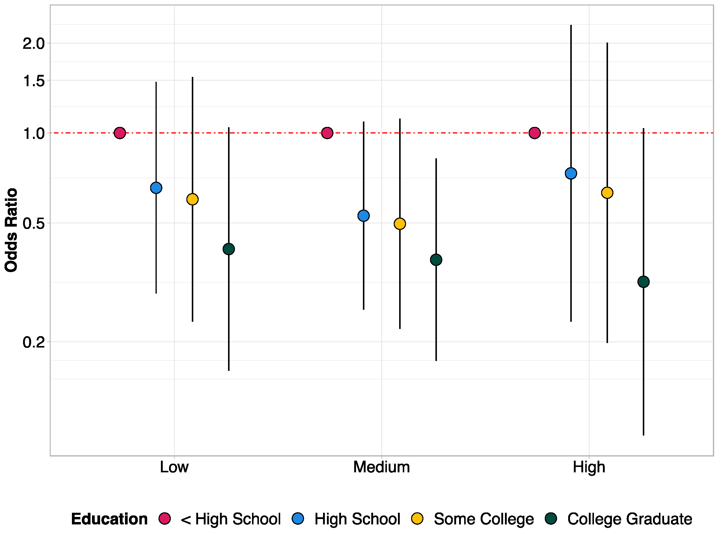
| Educational Attainment | ||
| Less than high school | 1.00 (Ref.) | |
| High school graduate | 0.63 (0.44; 0.90) | 0.012 * |
| Some college or equivalent | 0.57 (0.38; 0.85) | 0.005 * |
| College graduate or higher | 0.36 (0.24; 0.53) | <0.001 * |
| Age (years) | ||
| 18–34 | 1.00 (Ref.) | |
| 35–49 | 3.07 (2.02; 4.66) | <0.001 * |
| 50–64 | 10.92 (7.57; 15.75) | <0.001 * |
| 65+ | 20.38 (13.82; 30.04) | <0.001 * |
| Sex | ||
| Male | 1.00 (Ref.) | |
| Female | 0.96 (0.78; 1.19) | 0.73 |
| Race/Ethnicity | ||
| NH White 1 | 1.00 (Ref.) | |
| NH Black 1 | 2.28 (1.79; 2.89) | <0.001 * |
| Hispanic/Latino | 1.17 (0.77; 1.76) | 0.465 |
| Other | 0.85 (0.53; 1.37) | 0.513 |
Publisher’s Note: MDPI stays neutral with regard to jurisdictional claims in published maps and institutional affiliations. |
© 2022 by the authors. Licensee MDPI, Basel, Switzerland. This article is an open access article distributed under the terms and conditions of the Creative Commons Attribution (CC BY) license (https://creativecommons.org/licenses/by/4.0/).
Share and Cite
Koh, C.; Kondo, M.C.; Rollins, H.; Bilal, U. Socioeconomic Disparities in Hypertension by Levels of Green Space Availability: A Cross-Sectional Study in Philadelphia, PA. Int. J. Environ. Res. Public Health 2022, 19, 2037. https://doi.org/10.3390/ijerph19042037
Koh C, Kondo MC, Rollins H, Bilal U. Socioeconomic Disparities in Hypertension by Levels of Green Space Availability: A Cross-Sectional Study in Philadelphia, PA. International Journal of Environmental Research and Public Health. 2022; 19(4):2037. https://doi.org/10.3390/ijerph19042037
Chicago/Turabian StyleKoh, Celina, Michelle C. Kondo, Heather Rollins, and Usama Bilal. 2022. "Socioeconomic Disparities in Hypertension by Levels of Green Space Availability: A Cross-Sectional Study in Philadelphia, PA" International Journal of Environmental Research and Public Health 19, no. 4: 2037. https://doi.org/10.3390/ijerph19042037
APA StyleKoh, C., Kondo, M. C., Rollins, H., & Bilal, U. (2022). Socioeconomic Disparities in Hypertension by Levels of Green Space Availability: A Cross-Sectional Study in Philadelphia, PA. International Journal of Environmental Research and Public Health, 19(4), 2037. https://doi.org/10.3390/ijerph19042037