Abstract
The reduction in locational traffic accident risks through appropriate traffic safety management is important to support, maintain, and improve children’s safe and independent mobility. This study proposes and verifies a method to evaluate the risk of elementary school students-vehicle accidents (ESSVAs) at individual intersections on residential roads in Toyohashi city, Japan, considering the difference in travel purposes (i.e., school commuting purpose; SCP or non-school commuting purpose: NSCP), based on a statistical regression model and Empirical Bayes (EB) estimation. The results showed that the ESSVA risk of children’s travel in SCP is lower than that in NSCP, and not only ESSVAs in SCP but also most ESSVAs in NSCP occurred on or near the designated school routes. Therefore, it would make sense to implement traffic safety management and measures focusing on school routes. It was also found that the locational ESSVA risk structure is different depending on whether the purpose of the children’s travels is SCP or NSCP in the statistical model. Finally, it was suggested that evaluation of locational ESSVA risks based on the EB estimation is useful for efficiently extracting locations where traffic safety measures should be implemented compared to that only based on the number of accidents in the past.
1. Introduction
Road traffic accidents are one of the major causes of death and disability among children over the world [1]. The threat of being involved in a traffic accident contains not only the risk of direct physical damage but also the long-term impact on children’s lifestyles. Namely, the greater the concern parents/guardians feel about traffic accidents involving their children, the less likely they are to allow their children to play freely outside or to go out independently without adults [2,3,4,5,6]. In fact, it has been reported that children’s opportunities to walk and cycle, and play outside, as well as children’s independent mobility (CIM), have decreased in the 21st century in some countries [7,8,9,10,11,12]. The decrease in daily walking and cycling opportunities leads to children’s lack of physical activity [7]. Children’s opportunities for physical activity are important for their physical maturation and the form of normal bone and behavior, and physical inactivity is widely recognized as one of the major risk factors in human health [8,13]. It has been argued that CIM is also important in fostering children’s autonomy and in curbing car-independent transportation style which reduces time lost by parents taking their children as well as traffic congestion [10]. Therefore, the reduction in traffic accident risks and threats through appropriate traffic safety management is very important in urban planning to support, maintain, and improve children’s safe and independent mobility (CSIM).
In traffic safety management, it is important to properly assess the risk of traffic accidents at each area or location, especially for identifying areas/locations where countermeasures should be implemented and verifying the effectiveness of those countermeasures. In previous studies on the evaluation of accident risk by areas/locations, statistical model analyses (so-called safety performance functions: SPF) have often been used to clarify the effects of various explanatory variables on the number of accidents [14]. Table 1 lists the main previous studies using a statistical modeling approach for the assessment of accident risk involving children by areas/locations [15,16,17,18,19,20]. The aggregation units for accident risk assessment are diverse, ranging from the microscopic level such as intersections and road segments to the macroscopic level such as prefectures. While these previous studies have made important contributions to the methodology for assessments of accident risks involving children by areas/locations, there have been issues to be dealt with.

Table 1.
Main previous studies using a statistical modeling approach for the assessment of accident risk involving children by areas/locations.
The first is the consideration of the children’s travel purposes. The risk of children walking and cycling being involved in accidents may be different between traveling for school commuting purposes (SCP) and traveling for non-school commuting purposes (NSCP). In Japan, children are expected to be safer on the road in SCP than in NSCP, because many elementary schools have adopted a group walking system, called “Shudan-togeko”, to and from schools, and parents/guardians and district communities provide generous safety support [21,22]. In recent years, several countries, including the United Kingdom, also have begun to implement group walking initiatives, called “Walking bus”, to school [21]. Thus, accident risk assessments that take into account the differences between children’s travel in SCP and in NSCP are internationally important. Inada et al. [20] analyzed traffic accidents involving elementary school students and junior high school students by prefecture in Japan, dividing the accidents into those involving the students in SCP and NSCP, and found that the number of killed or seriously injured (KSI) cases during travels in SCP was approximately 30–40% lower than that during travels in NSCP. However, the study was conducted only at the macro level (i.e., prefecture-level), and, to the best of the author’s knowledge, there have been no studies in which whether the children’s purpose was SCP or NCSP was taken into account in a micro level (such as intersections or road segments level) analysis.
As the second issue, the accident risk of each location may be affected by a great variety of factors specific to the location. It is difficult to incorporate all of the factors as explanatory variables in a statistical model, and the effects of factors other than the explanatory variables are represented as the error term with a probability distribution. Therefore, in assessing accident risks at different locations, it is necessary to properly consider the balance between the average effects of explanatory variables and the effect of location-specific characteristics. While the Empirical Bayesian (EB) estimation method has been proposed and used in the context of a before–after study on the evaluation of traffic safety measures [23,24,25,26,27,28,29,30], it is also applicable to the purpose of extracting locations where countermeasures should be implemented by properly evaluating the accident risks at individual locations [31,32,33,34,35,36,37]. Although there have been some previous studies applying the EB method to evaluate the locational risks of accidents involving general pedestrian [30,33], no studies applying the EB method to assess the locational risks of accidents involving children have been seen.
Therefore, this study proposes and verifies a method to evaluate the risk of vehicle–children accidents at individual intersections on residential roads in Toyohashi city, Japan, considering the difference in travel purposes (i.e., SCP or NSCP), based on a statistical regression model and EB estimation.
2. Materials and Methods
2.1. Target Area
The target area was the entire Toyohashi City, Aichi Prefecture, Japan. There are 52 elementary schools in the city (see Figure 1), and the number of elementary school students is approximately 20,000 as of 2018. Almost all the students walk to school, except for about 10 students who cycle to school.
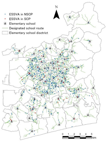
Figure 1.
Locations of ESSVAs and designated school routes in the target area.
2.2. Data
2.2.1. Traffic Accident Data
The accident data used in this study were police-reported elementary school student-vehicle accidents (ESSVAs: injury accidents in which the first or second party was an elementary school student while walking or cycling) that occurred in Toyohashi City over a 12-year period from 2009 to 2020 (totally 638 ESSVAs). The individual accident data include the children’s travel purpose (i.e., SCP or NSCP). Figure 1 shows the distribution of the locations of the ESSVAs by the children’s travel purpose.
The ESSVAs which occurred within a radius of 50 m from the center of each community street intersection were extracted as “intersection ESSVAs”, which were 360 ESSVAs (56.4% of all the ESSVAs). The community street intersections were defined as intersections with three or more legs of community streets other than “national expressways”, “general national highways”, “major regional roads”, “general prefectural roads”, and “major general roads” in the road network data of Zmap-Area II (ZENRIN corp.). Of the 7719 target intersections, one ESSVA occurred at 296 (3.8%) intersections, two ESSVAs at 24 (0.31%) intersections, three ESSVAs at four (0.052%) intersections, and four ESSVAs at one (0.013%) intersection, during the 12-year period.
We used the 299 ESSVAs in the first nine years as the “risk estimation period” to estimate the ESSVA risk at each intersection, and the 61 ESSVAs in the last three years as the “evaluation period” to evaluate the results of the estimation.
2.2.2. Risk Exposure Data
Accident risk exposure is an important factor for the statistical model analysis of locational accident risks, and some studies have made efforts to measure exposure for evaluating the locational risk of accidents involving pedestrians [38,39,40,41]. In this study, the exposure should be the number of passings or activities of elementary school students at each intersection. However, it is difficult to measure these data over the wide city area. As shown in Table 1, the previous studies have tried to estimate exposure by children population [18,20], by questionnaire surveys asking about travel routes [16,17], by an observation survey of travel mode to schools [19], and by a journey allocation model based on shortest routes [16].
On the other hand, the author and the Toyohashi City Board of Education have collaboratively georeferenced the designated school route data (see Figure 1) and the gathering point data, with the number of elementary school students for each school commuting group in the city. In this study, based on the designated school route data (2018 version), we calculated the following indices as surrogate variables for ESSVA risk exposure at the intersections [42]:
- Number of elementary school students on the surrounding school routes (NSSR15, 50, 100): the number of elementary school students on the designated school route that passes within a radius of 15 m, 50 m, or 100 m from the center of each target intersection;
- Number of elementary school students at the surrounding gathering points (NSGP15, 50, 100): the number of elementary school students at the gathering points located within a radius of 15 m, 50 m, or 100 m from the center of each target intersection;
- Distance to the nearest school route (DSR): the distance from the center of each intersection to the nearest designated school route.
Note that there are no major differences in the designated school route data in recent years.
2.2.3. Other Data
The ESSVA risk at an intersection is also may be greatly affected by the vehicle traffic volume [16,43,44]. Therefore, in order to take into account the effect of vehicle traffic volume at each target intersection, this study used probe vehicle data corrected by Pioneer Corp. for the years 2016–2019. The validity of the probe vehicle data has been confirmed in our previous studies [30]. The probe vehicle traffic volumes of all legs in the direction of inflow to the intersection were summed up to obtain the probe vehicle traffic volume for each target intersection, which was used as a variable to represent the vehicle traffic volume.
As other explanatory variables for road traffic environment conditions, we used the number of legs for each intersection, the presence or absence of traffic signals, the urban area land use type by 1/10 mesh (100 m mesh) of the National Land Information, whether each intersection is within the densely inhabited district (DID), and the distance to the nearest park.
2.3. Statistical Model
In this study, the locational accident risk is defined as the expected value of the number of ESSVAs by intersections in a specific period. Therefore, a count data model is used as the statistical model. The Poisson regression model is the simplest count data model. However, because the error structure (i.e., Poisson distribution) has a strong limitation that the variance equals the expected value, the negative binomial (NB) regression model, which is one of the extensions of the Poisson regression model, is commonly applied in recent accident count data modeling [14]. Additionally, in this study, the NB regression model is used.
To the best of the author’s knowledge, the EB estimation has been found in the field of traffic accident risk assessment since Gipps [23], Abbess et al. [24], and Jarrett et al. [31] in the early 1980s, and later it was well-organized by Hauer [25] in the context of before/after study of traffic safety measures. In order to summarize the method for assessing accident risk considering location-specific factors using the EB estimation, it is first explained that the Poisson regression model can be extended to the NB regression model by assuming the property that the expected value in the Poisson regression model itself varies stochastically according to the gamma distribution. Then, the EB method is presented for the evaluation of the risk of accidents at each location, taking into account the location-specific effects that cannot be explained by the average effects (fixed effects) of the explanatory variables considered in the model.
2.3.1. Poisson Regression Model
Suppose that the number of accidents at location during a certain period of time follows a Poisson distribution with an expected value that is a function of the explanatory variable vector and the corresponding parameter vector :
Thus, the probability that accidents occur at location during the period is
and the expected value and variance of are
where
2.3.2. Accident Risk Evaluation That Considers Location-Specific Factors
Assuming that the expected value of the Poisson regression model described above is not completely determined only by the function of explanatory variables and parameters, but is also affected by factors specific to location , and then assuming as an alternative to the expected value the random variable which follows a gamma distribution with the shape parameter and the rate parameter :
The probability that be a certain value is
and the expected value and variance of are
The structure that the expected value of the number of accidents is determined following the gamma distribution, and the realization of the number of accidents occurs following the Poisson distribution with as the parameter can be interpreted as a hierarchical model. Therefore, under the information that accidents actually occurred at location , the probability that is a certain value can be obtained by Bayes’ theorem:
Here, and are the prior parameters. Furthermore, the gamma distribution is the natural conjugate distribution of the Poisson distribution, thus it is known that the posterior distribution is also gamma, so that:
and its expected value is
The expected value of can be used as an accident risk evaluation index that takes into account location-specific factors.
2.3.3. EB Estimation through an NB Regression Model
The accident risk evaluation index in Equation (11) depends on the prior parameters and . Therefore, in this study, these prior parameters are estimated by the EB method. That is, we use and which maximize the marginal likelihood:
Expanding Equation (12) further and setting , we obtain:
indicating that follows an NB distribution with parameters and :
The expected value and variance of are
Here, is called the dispersion parameter. The larger , the smaller the variance (residual deviation) of . When , the variance is equal to the expected value, which means that the NB distribution is consistent with the Poisson distribution.
From the above, the EB estimation of is possible by estimating the NB regression model using the actual number of accidents by locations and the explanatory variable vector , and then by using the variance parameter and the expected number of accidents by location obtained from the estimated NB regression model as prior parameters. Denoting the EB estimator of as , it can be shown that,
Therefore, it can be found that this EB estimator is a weighted average of the two variables: (1) the expected number of accidents , which is calculated based on the average effects of the explanatory variables in the estimated NB regression model; and (2) the number of accidents that actually occurred. It can be also found that the larger the dispersion parameter of the NB regression model is (i.e., the smaller the residual deviation by the NB regression model is), the greater the weight is given to . According to Ghosh and Meeden [45], “one of the main features of EB analysis is to borrow strength from the ensemble; that is, use information from similar sources in constructing estimators and predictors in addition to the most directly available source of information.”
Therefore, this study first estimated the parameter and the dispersion parameter of the NB regression model shown in Equations (4) and (14), using the actual number of ESSVAs at each intersection (explained in Section 2.2.1) as the objective variable and the risk exposure indices (explained in Section 2.2.2) and other road traffic environment conditions (explained in Section 2.2.3) as explanatory variables . Next, using the explanatory variables and the estimated model parameter , the NB estimate of the expected number of ESSVAs at each intersection, , was calculated by Equation (4). Then, using the NB estimate of the expected number of ESSVAs, the actual number of ESSVAs , and the parameter , the EB estimate of the expected number of ESSVAs at each intersection, , was calculated by Equation (17). This EB estimate of the expected number of ESSVAs was the risk evaluation value for each intersection.
2.4. Evaluation of Efficiency to Extract Risky Locations
To evaluate the usefulness of the EB estimation from the view of efficient extraction of high ESSVA risk locations, we calculated efficiency criteria by the following procedure. The concept of efficiency here is that “the higher the number of ESSVAs in the evaluation period per one extracted ESSVA risk intersection, the higher the efficiency”.
- Each location was ranked in order of riskiness based on the three criteria, respectively:
- Actual number criterion, i.e., the higher the actual number of ESSVAs in the risk estimation period (the first nine years), the higher the risk is;
- NB estimate criterion, i.e., the higher the expected number of ESSVAs calculated by the NB regression model, the higher the risk is;
- EB estimate criterion, i.e., the higher the expected number of ESSVAs corrected by the EB estimation method, the higher the risk is.
- Based on the rankings of the three criteria, the cumulative sums of the actual number of ESSVAs in the evaluation period (the last three years) up to the rank were, respectively calculated.
- The cumulative sums of the actual number of ESSVAs in the evaluation period for the three criteria were, respectively divided by the number of intersections up to the rank, which is the efficiency in this study.
Figure 2 illustrates the flow of this study described so far.
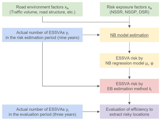
Figure 2.
The flow of this study.
3. Results
3.1. Aggregation Analyses
Figure 3 shows the distribution of the occurrence time of ESSVAs by the children’s travel purposes, indicating that many of the ESSVAs occurred in the time period of 4:00–5:00 p.m. in NSCP. The high number of ESSVAs occurring in NSCP at this time means that elementary school students are mostly involved in an accident when being out to play or go somewhere (e.g., friends’ houses or shops) after returning home on weekdays or on holidays.
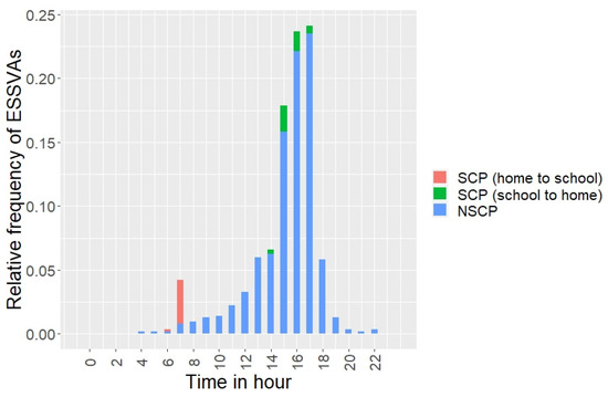
Figure 3.
Time distribution of the occurrences of ESSVAs in the target area by travel purpose.
Figure 4 shows the distribution of the occurrence of ESSVAs regarding the distance from the nearest school route by the children’s travel purposes. As expected, most (roughly 80%) of the ESSVAs in SCP occurred on the school routes since children basically walk to school and walk back home along the designated school routes. On the other hand, it is a surprise that most ESSVAs in NSCP also occurred on or close to (roughly within 100 m of) the school routes. This could be an important fact and will be discussed, along with the statistical model estimation results below, in detail in Section 4.
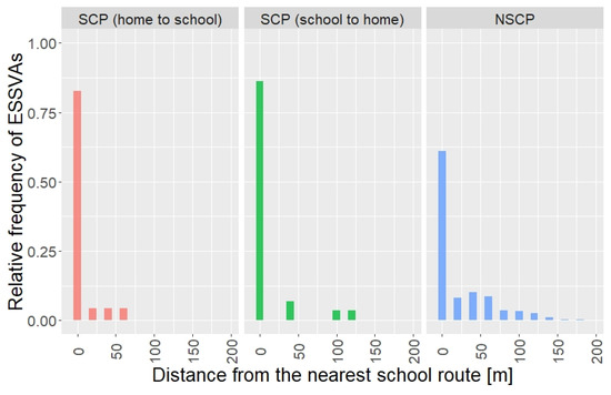
Figure 4.
Distribution of the occurrences of ESSVAs in target area by the distance from the nearest school route and travel purpose.
3.2. Estimation Results of the NB Regression Model
Table 2 shows the estimation results of two types of final NB regression models using the numbers of ESSVAs in SCP and the numbers of ESSVAs in NSCP, at the target intersections in the risk estimation period as the objective variable. They indicated that the statistically significant explanatory variables were different between the SCP model and the NSCP model.
Table 2.
Estimation results of the NB regression models for the ESSVAs.
The parameter of the constant term in the SCP model was strongly lesser than those in the other models, indicating that children’s risk to be involved in an accident during school commuting is very lower than during other travels.
Regarding the surrogate variables for the ESSVA risk exposure, the more the number of elementary school students on the designated school route passing within the intersections (NSSR15), the higher the ESSVA risk was in the SCP model. In the NSCP model, on the other hand, the nearer the distance from the intersections to the nearest designated school route, the higher the ESSVA risk was. These results suggest that the designated school route data could be useful as surrogate variables for ESSVA risk exposure indicators.
As for the other explanatory variables, the main findings were as follows:
- ESSVA risk increased with vehicle traffic volume in both models, but the impact was less in the SCP model than in the NSCP model;
- ESSVA risk was higher at four-leg intersections than at three-leg intersections in the NCSP model, but there was no such effect of road structure in the SCP model;
- The SCP model showed a lower ESSVA risk at intersections near parks, but the NCSP model did not show such an effect;
- ESSVA risk was higher in areas with building use in both models, but was particularly strong in the SCP model;
- Intersections within the DID had lower ESSVA risk in the SCP model, but the effect is not shown in the NSCP model.
3.3. Results of the EB Estimation
Figure 5 shows the scatter charts plotting the ESSVA risks calculated by the NB regression model () on the horizontal axes and those corrected by the EB estimation () on the vertical axes, according to the number of ESSVAs actually occurred during the risk estimation period shown at the top of the charts (0–3). The 45-degree line is also plotted. It can be seen that in the chart for the intersections where the actual numbers of ESSVAs were zero (the leftmost chart in Figure 5), all points were below the 45-degree line. This means that the expected numbers of ESSVAs were adjusted downward through the EB estimation because the actual numbers of ESSVAs had been smaller than the expected numbers estimated by the NB model. On the other hand, in the chart for the intersections where the actual numbers of ESSVAs were two or three (the right two charts in Figure 5), all points were above the 45-degree line. This means that the expected numbers of ESSVAs were adjusted upward through the EB estimation because the actual numbers of ESSVAs had been greater than the expected numbers estimated by the NB model. Additionally, in the chart for the intersections where the actual numbers of ESSVAs were one (the second left chart in Figure 5), the downward and upward adjustments described above were mixed. It can also be seen that even for the intersections with the same actual numbers of ESSVAs, the further to the right, the greater the difference between each point and the 45-degree line tended to be. This means that the higher the ESSVA risks calculated by the NB regression model were, the larger the magnitude of the adjustment by the EB estimation was.
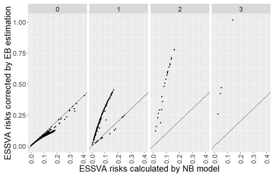
Figure 5.
Comparison of ESSVA risks (the expected numbers of ESSVAs) according to the actual number of ESSVAs (0–3 from left to right) in the risk estimation period (nine years).
Figure 6 shows the efficiencies calculated by the procedure explained in Section 2.4 based on the three criteria. It can be seen that the actual number criterion had the highest efficiency up to the 6th ESSVA risk rank, whereas the EB estimate criterion had the highest efficiency from the 7th up to about the 60th risk rank. This means that, in this study case, while using the actual number of ESSVAs was more efficient in extracting the top six risky locations, using the EB estimation was more efficient in extracting the risky locations beyond these six locations.
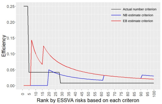
Figure 6.
Comparison of the efficiencies for risky location extraction among the three criteria.
4. Discussion and Conclusions
The results of the aggregation analyses and the statistical model analysis showed that ESSVAs in SCP are less frequent than those in NSCP. This tendency is similar throughout Japan [20], and this may be due in large part to the effect of the cultural safety systems such as group school commuting (called “shudan-togeko”) and the safety supports such as crossing guard by district communities when traveling in SCP, as suggested by Waygood et al. [21] and Matsuo et al. [22] in macroscopic levels. Rothman et al. [19] showed a different result that intersections with school crossing guards had higher collision risk. However, there is a possibility that the locations where school crossing guards are located reflect the areas where many children walk, namely the risk exposure is higher resulting in higher accident frequencies. The result in this study is considered reasonable because the amount of risk exposure in SCP used in this is valid as described below.
The results of the aggregation analysis revealed that not only ESSVAs in SCP but also most ESSVAs in NSCP occurred on or near the designated school routes. The statistical model analysis showed that the number of elementary students commuting to school on each designated school route passing within a radius of 15 m from the center of each target intersection (NSSR15) was significant in the SCP model. This can be interpreted as the number of children passing through the designated school routes functioning as a risk exposure variable for ESSVAs in SCP. This is precisely because the number of children commuting to school on the school route itself is appropriate as exposure for ESSVA risk in SCP. Lee et al. [17] showed similar results using the number of children on the route to school based on a questionnaire survey as an exposure variable. On the other hand, in the NSCP model, the distance from each intersection to the nearest school route (DSR) was significant, indicating that the structure regarding ESSVA risk exposure differs depending on the children’s travel purposes. This result suggests that elementary school students tend to use the designated school routes even for NSCP because they are familiar with the school routes due to daily use in SCP, resulting that the number of ESSVAs on or near school routes would be higher. Therefore, even though the fact described above is that the majority of the ESSVAs occurred while walking and cycling for NSCP, it would make sense to implement traffic safety management and measures focusing on school routes as the Japanese national and regional government currently makes efforts [46].
As Bennet and Yiannakoulias [16] showed, ESSVA risk increased with vehicle traffic volume. However, the impact was less in the SCP model than in the NSCP model. This may be because there is a cultural system that contributes to the safety of children traveling to and from school in Japan, as mentioned above, and also because crossing guards are present especially in locations with heavy vehicle traffic. On the other hand, it suggests that traffic calming is more important for the safety of children traveling in NCSP. Many previous studies showed the safety effect of traffic calming devices on residential roads [47,48].
Although some previous studies used the number of legs of intersections but could not find a significant effect [17,18], this study found that ESSVA risk was higher at four-leg intersections than at three-leg intersections for NCSP travels. While the result that ESSVA risk was higher in areas with building use in both models is similar to the previous studies [15,16,17,19], this study additionally found that the effect was particularly strong for SCP travels. Inada et al. [20] showed that locations of DID have the effect of an increase in children’s accident risk through the prefectural level macroscopic analyses; however, this study revealed that the intersections within the DID have lower ESSVA risk for SCP travels. This may be because the size of group commuting and safety support by district communities, as described above, are more extensive in densely populated areas. As mentioned so far, the locational ESSVA risk structure, including the exposure, varies depending on whether the purpose of the children’s travels is SCP or NSCP, which is considered an important finding of this study.
Regarding the EB estimation results, it was shown that in this study case, using the EB estimate criterion was more efficient when extracting more than six risky locations. This suggested that the evaluation of locational accident risks based on the EB estimation is useful also for efficiently extracting locations where traffic safety measures for ESSVAs should be implemented compared to that only based on the number of accidents in the past, as argued in the previous studies applying EB method for other types of accidents [33,34,35,36,37]. In practice, it would be better to use both the number of accidents and the EB estimation method to identify risky locations.
Finally, this study has some limitations and further issues. The first is that the exposure data for locational ESSVA risks in NSCP were insufficient. While we used designated school route data as a surrogate variable for exposure in this study, the spatial distribution of children’s travels and activities in NSCP should be measured and used in some way (e.g., questionnaire/diary survey [15,17], observation survey [19], GPS logger survey [49], etc.).
The second is to be able to assess in detail the safety effects of group commuting and safety support by district communities. For this purpose, it is necessary to make comparisons between districts with different approaches to safety support, and between elementary school districts with and without group commuting.
Thirdly, although the same statistical modeling and predicting approach (i.e., NB regression model and EB estimation method) can be used for other regions and countries, the road traffic environment conditions and data availability differ among regions or countries. Therefore, it is necessary to consider an objective variable and a variety of explanatory variables including risk exposure indicators by tailoring them to those conditions.
Author Contributions
Conceptualization, K.M. (Kojiro Matsuo); methodology, K.M. (Kojiro Matsuo); software, K.M. (Kojiro Matsuo); validation, K.M. (Kojiro Matsuo), K.M. (Kosuke Miyazaki) and N.S.; formal analysis, K.M. (Kojiro Matsuo); investigation, K.M. (Kojiro Matsuo); resources, K.M. (Kojiro Matsuo); data curation, K.M. (Kojiro Matsuo); writing—original draft preparation, K.M. (Kojiro Matsuo); writing—review and editing, K.M. (Kojiro Matsuo), K.M. (Kosuke Miyazaki) and N.S.; visualization, K.M. (Kojiro Matsuo); supervision, K.M. (Kojiro Matsuo) and N.S.; project administration, K.M. (Kojiro Matsuo); funding acquisition, K.M. (Kojiro Matsuo) and K.M. (Kosuke Miyazaki). All authors have read and agreed to the published version of the manuscript.
Funding
This research was funded by the Japan Society for the Promotion of Science (JSPS) under the Grant-in-Aid for Scientific Research (C) 20K04743 and Toyohashi University of Technology under the Cooperative Project for Innovative Research 2-1.
Institutional Review Board Statement
Not applicable.
Informed Consent Statement
Not applicable.
Data Availability Statement
Not applicable.
Acknowledgments
The authors would like to express their gratitude to Aichi Prefectural Police for providing the traffic accident data and to Toyohashi City Government for providing the designated school route data, respectively, used in this study.
Conflicts of Interest
The authors declare no conflict of interest.
References
- World Health Organization. Youth and Road Safety; World Health Organization: Geneva, Switzerland, 2007. [Google Scholar]
- Kerr, J.; Rosenberg, D.; Sallis, J.F.; Saelens, B.E.; Frank, L.D.; Conway, T.L. Active commuting to school: Associations with environment and parental concerns. Med. Sci. Sport. Exerc. 2006, 38, 787–794. [Google Scholar] [CrossRef] [PubMed]
- Timperio, A.; Ball, K.; Salmon, J.; Roberts, R.; Giles-Corti, B.; Simmons, D.; Baur, L.A.; Crawford, D. Personal, family, social, and environmental correlates of active commuting to school. Am. J. Prev. Med. 2006, 30, 45–51. [Google Scholar] [CrossRef] [PubMed]
- Carver, A.; Timperio, A.; Hesketh, K.; Crawford, D. Are children and adolescents less active if parents restrict their physical activity and active transport due to perceived risk? Soc. Sci. Med. 2010, 70, 1799–1805. [Google Scholar] [CrossRef]
- Napier, M.A.; Brown, B.B.; Werner, C.M.; Gallimore, J. Walking to school: Community design and child and parent barriers. J. Environ. Psychol. 2011, 31, 45–51. [Google Scholar] [CrossRef]
- Fallah Zavareh, M.; Abolhasannejad, V.; Mamdoohi, A.; Nordfjærn, T. Barriers to children’s walking to school in Iranian and Chinese samples. Transp. Res. Part F Traffic Psychol. Behav. 2020, 73, 399–414. [Google Scholar] [CrossRef]
- Cooper, A.R.; Andersen, L.B.; Wedderkopp, N.; Page, A.S.; Froberg, K. Physical activity levels of children who walk, cycle, or are driven to school. Am. J. Prev. Med. 2005, 29, 179–184. [Google Scholar] [CrossRef]
- Rosenberg, D.E.; Sallis, J.F.; Conway, T.L.; Cain, K.L.; McKenzie, T.L. Active transportation to school over 2 years in relation to weight status and physical activity. Obesity 2006, 14, 1771–1776. [Google Scholar] [CrossRef] [PubMed]
- Nevelsteen, K.; Steenberghen, T.; Van Rompaey, A.; Uyttersprot, L. Controlling factors of the parental safety perception on children’s travel mode choice. Accid. Anal. Prev. 2012, 45, 39–49. [Google Scholar] [CrossRef]
- Shaw, B.; Bicket, M.; Elliott, B.; Fagan-Watson, B.; Mocca, E.; Hillman, M. Children’s Independent Mobility: An International Comparison and Recommendations for Action; Policy Studies Institute: London, UK, 2015. [Google Scholar]
- Waygood, E.O.D.; Susilo, Y.O. Walking to school in Scotland: Do perceptions of neighbourhood quality matter? IATSS Res. 2015, 38, 125–129. [Google Scholar] [CrossRef]
- Xu, X.; Taniguchi, A.; Ishigami, T.; Hirata, S. The Current Status and Transition of Japanese Children’s Travel Behavior. In Proceedings of the Infrastructure Planning 51, Fukuoka, Japan, 6–7 June 2015. [Google Scholar]
- World Health Organization. Global Recommendation on Physical Activity for Health; World Health Organization: Geneva, Switzerland, 2010. [Google Scholar]
- Lord, D.; Mannering, F. The statistical analysis of crash-frequency data: A review and assessment of methodological alternatives. Transp. Res. Part A Policy Pract. 2010, 44, 291–305. [Google Scholar] [CrossRef]
- Elias, W.; Shiftan, Y. Analyzing and modeling risk exposure of pedestrian children to involvement in car crashes. Accid. Anal. Prev. 2014, 62, 397–405. [Google Scholar] [CrossRef]
- Bennet, S.A.; Yiannakoulias, N. Motor-vehicle collisions involving child pedestrians at intersection and mid-block locations. Accid. Anal. Prev. 2015, 78, 94–103. [Google Scholar] [CrossRef] [PubMed]
- Lee, G.; Park, Y.; Kim, J.; Cho, G.-H. Association between intersection characteristics and perceived crash risk among school-aged children. Accid. Anal. Prev. 2016, 97, 111–121. [Google Scholar] [CrossRef] [PubMed]
- Hwang, J.; Joh, K.; Woo, A. Social inequalities in child pedestrian traffic injuries: Differences in neighborhood built environments near schools in Austin, TX, USA. J. Transp. Health 2017, 6, 40–49. [Google Scholar] [CrossRef]
- Rothman, L.; Howard, A.; Buliung, R.; Macarthur, C.; Richmond, S.A.; Macpherson, A. School environments and social risk factors for child pedestrian-motor vehicle collisions: A case-control study. Accid. Anal. Prev. 2017, 98, 252–258. [Google Scholar] [CrossRef] [PubMed]
- Inada, H.; Tomio, J.; Ichikawa, M.; Nakahara, S. Regional disparities in road traffic injury rates involving elementary and junior high school children while commuting among Japan’s 47 prefectures between 2004 and 2013. Accid. Anal. Prev. 2019, 125, 79–84. [Google Scholar] [CrossRef] [PubMed]
- Waygood, O.; Taniguchi, A.; Craig-St-Louis, C.; Xu, X. International Origins of Walking School Buses and Child Fatalities in Japan and Canada. Traffic Sci. 2015, 46, 30–42. [Google Scholar]
- Matsuo, K.; Ibrahim, N.D.; Miyazaki, K.; Sugiki, N. A Macroscopic Analysis of the Traffic Safety Effects of Group School Commuting for Elementary School Students. In Proceedings of the Infrastructure Planning 64, Online, 3–5 December 2021. [Google Scholar]
- Gipps, P.G. Examining the Safety Contributions of Traffic Control Devices. Transport Research for Social and Economic Progress. In Proceedings of the Second World Conference on Transport Research, London, UK, 14–17 April 1980; pp. 2604–2609. [Google Scholar]
- Abbess, C.; Jarrett, D.; Wright, C.C. Accidents at blackspots: Estimating the effectiveness of remedial treatment, with special reference to the “regression-to-mean” effect. Traffic Eng. Control 1981, 22, 535–542. [Google Scholar]
- Hauer, E. Observational Before/After Studies in Road Safety: Estimating the Effect of Highway and Traffic Engineering Measures on Road Safety; Emerald Publishing: London, UK, 1997; pp. 175–218. [Google Scholar]
- Hauer, E.; Harwood, D.W.; Council, F.M.; Griffith, M.S. Estimating safety by the Empirical Bayes method: A tutorial. Transp. Res. Rec. 2002, 1784, 126–131. [Google Scholar] [CrossRef]
- Ko, M.; Geedipally, S.R.; Walden, T.D.; Wunderlich, R.C. Effects of red light running camera systems installation and then deactivation on intersection safety. J. Saf. Res. 2017, 62, 117–126. [Google Scholar] [CrossRef]
- Tang, H.; Gayah, V.V.; Donnell, E.T. Crash modification factors for adaptive traffic signal control: An Empirical Bayes before-after study. Accid. Anal. Prev. 2020, 144, 105672. [Google Scholar] [CrossRef] [PubMed]
- Wood, J.; Donnell, E.T. Empirical Bayes before-after evaluation of horizontal curve warning pavement markings on two-lane rural highways in Pennsylvania. Accid. Anal. Prev. 2020, 146, 105734. [Google Scholar] [CrossRef] [PubMed]
- Matsuo, K.; Chigai, N.; Chattha, M.I.; Sugiki, N. Vulnerable road user safety evaluation using probe vehicle data with collision warning information. Accid. Anal. Prev. 2022, 165, 106528. [Google Scholar] [CrossRef] [PubMed]
- Jarrett, D.F.; Abbess, C.; Wright, C.C. Bayesian Methods Applied to Road Accident Black Spot Studies: Some Recent Progress; Institute for Road Safety Research (SWOV): Hague, The Netherlands, 1982; pp. 69–74. [Google Scholar]
- Hauer, E. Empirical Bayes approach to the estimation of “unsafety”: The multivariate regression method. Accid. Anal. Prev. 1992, 24, 457–477. [Google Scholar] [CrossRef]
- Ng, K.S.; Hung, W.T.; Wong, W.G. An algorithm for assessing the risk of traffic accident. J. Saf. Res. 2002, 33, 387–410. [Google Scholar] [CrossRef]
- Montella, A. A comparative analysis of hotspot identification methods. Accid. Anal. Prev. 2010, 42, 571–581. [Google Scholar] [CrossRef] [PubMed]
- Lee, J.; Chung, K.; Kang, S. Evaluating and addressing the effects of regression to the mean phenomenon in estimating collision frequencies on urban high collision concentration locations. Accid. Anal. Prev. 2016, 97, 49–56. [Google Scholar] [CrossRef]
- Yang, B.Z.; Loo, B.P.Y. Land use and traffic collisions: A link-attribute analysis using Empirical Bayes method. Accid. Anal. Prev. 2016, 95, 236–249. [Google Scholar] [CrossRef] [PubMed]
- Chattha, M.I.; Matsuo, K.; Sugiki, N. Risk Analysis of Pedestrian and Bicycle Accidents at Intersections in Toyohashi City Using Empirical Bayes Method. J. East. Asia Soc. Transp. Stud. 2022, 14, 2093–2112. [Google Scholar]
- Lam, W.W.Y.; Yao, S.; Loo, B.P.Y. Pedestrian exposure measures: A time-space framework. Travel Behav. Soc. 2014, 11, 22–30. [Google Scholar] [CrossRef]
- Yao, S.; Loo, B.P.; Lam, W.W. Measures of activity-based pedestrian exposure to the risk of vehicle-pedestrian collisions: Space-time path vs. potential path tree methods. Accid. Anal. Prev. 2015, 75, 320–332. [Google Scholar] [CrossRef] [PubMed]
- Papadimitriou, E. Towards an integrated approach of pedestrian behaviour and exposure. Accid. Anal. Prev. 2016, 92, 139–152. [Google Scholar] [CrossRef] [PubMed]
- Xie, S.Q.; Dong, N.; Wong, S.C.; Huang, H.; Xu, P. Bayesian approach to model pedestrian crashes at signalized intersections with measurement errors in exposure. Accid. Anal. Prev. 2018, 121, 285–294. [Google Scholar] [CrossRef] [PubMed]
- Sahdan, H.; Matsuo, K.; Sugiki, N. Statistical Model Analyses of Traffic Accidents Involving Elementary Students at Intersections Considering Exposure Factors. In Proceedings of the 12th International Symposium on City Planning and Environment Management in Asian Countries, Seoul, Korea, 1–4 November 2019. [Google Scholar]
- Davis, G.A. Method for estimating effect of traffic volume and speed on pedestrian safety for residential streets. Transp. Res. Rec. 1998, 1636, 110–115. [Google Scholar] [CrossRef]
- Wang, Y.; Kockelman, K.M. A Poisson-lognormal conditional-autoregressive model for multivariate spatial analysis of pedestrian crash counts across neighborhoods. Accid. Anal. Prev. 2013, 60, 71–84. [Google Scholar] [CrossRef] [PubMed]
- Ghosh, M.; Meeden, G. Empirical Bayes estimation in finite population sampling. J. Am. Stat. Assoc. 1986, 81, 1058–1062. [Google Scholar] [CrossRef]
- Japan Cabinet Office, Government of Japan. Securing Traffic Safety in School Roads. In White Paper on Traffic Safety in Japan 2014; Japan Cabinet Office, Government of Japan: Tokyo, Japan, 2015. [Google Scholar]
- Jones, S.J.; Lyons, R.A.; John, A.; Palmer, S.R. Traffic calming policy can reduce inequalities in child pedestrian injuries: Database study. Inj. Prev. 2005, 11, 152–156. [Google Scholar] [CrossRef] [PubMed]
- Matsuo, K.; Sugihara, M.; Yamazaki, M.; Mimura, Y.; Yang, J.; Kanno, K.; Sugiki, N. Hierarchical Bayesian modeling to evaluate the impacts of intelligent speed adaptation considering individuals’ usual speeding tendencies: A correlated random parameters approach. Anal. Methods Accid. Res. 2020, 27, 100125. [Google Scholar] [CrossRef]
- Nguyen, A.; Borghese, M.M.; Janssen, I. Pedestrian traffic safety and outdoor active play among 10–13 year olds living in a mid-sized city. Prev. Med. Rep. 2018, 10, 304–309. [Google Scholar] [CrossRef] [PubMed]


Publisher’s Note: MDPI stays neutral with regard to jurisdictional claims in published maps and institutional affiliations. |
© 2022 by the authors. Licensee MDPI, Basel, Switzerland. This article is an open access article distributed under the terms and conditions of the Creative Commons Attribution (CC BY) license (https://creativecommons.org/licenses/by/4.0/).