
Geospatial Correlation Analysis between Air Pollution Indicators and Estimated Speed of COVID-19 Diffusion in the Lombardy Region (Italy)

 ,
,  ,
, 
Abstract
:1. Introduction
- (1)
- Data reliability: It is widely recognized that the official data relevant to COVID-19 were underestimating its actual diffusion [21,29,30,31], and this was particularly true when considering Italy during the first pandemic peak (March–April 2020, ISTAT, https://www.istat.it/it/archivio/245415, last access on 3 November 2021): immediately after the first confirmed case, screening protocols were arranged in an attempt to understand the contagion line, tracing back all contacts of people positive to tests but, after few days, when the recorded cases exceeded tracing possibilities [32], testing started to be performed (according to limited capabilities) only to people showing compatible symptoms with COVID-19. Still, diagnosis capabilities were quickly saturated, and the swab test for COVID-19 was performed for the most severe patients only [33,34].
- (2)
- Confounding factors: As clearly stated in a letter to the editors by Riccò et al. [35], it is possible that, studying the relationship between air pollution and COVID-19 cases, ‘we are observing a correlation rather than a causation’. The use of territorial subdivisions for administrative purposes may force the comparison of areas with significant socio-economic disparities, which is likely to be a much more relevant factor (compared to pollution) when assessing the speed of diffusion of the pandemic. Therefore, Riccò et al. suggested that ‘a more appropriate way in dealing with and understanding the relationship between air pollution and SARS-CoV-2 infection incidence rates may occur comparing geographical areas characterized by similar socio-economic development, but strikingly different environmental status (e.g., highly polluted areas versus those with low pollution levels)’. Some studies [13,14,17,20,21,23,26] did take into account possible confounding factors (as suggested by the literature [29]), such as population density [13,20,26], population age [13,14,20,26], socio-economic status [20,23,26], ethnicity [20], people mobility [17,20], and healthcare resources [20,23].
- (3)
- Lockdown-related biases: As once again stated by Riccò et al. [35], ‘it should be stressed that lockdown measures are significantly affecting air pollutants, reducing their daily concentrations’. The comparison of territories where lockdown measures were established at very different epidemic phases (a widely applied approach, especially in studies relevant to the Italian territory) lacks in meaningfulness, as the impact of complete lockdown measures heavily affects both phenomena under analysis (COVID-19 epidemic and air pollution).
- Diffusion of the pandemic could be inferred by the analysis of georeferenced Emergency Medical Services (EMS) interventions (ambulances dispatches) for respiratory problems, which is an approach we recently proposed and validated [36]. Such indirect data are not biased by testing policies and management strategies, which instead affected consistently the reliability of official data, especially in the very first phases of the pandemic.
- A comparison among areas having very similar territorial and socio-economic characteristics within the Lombardy region could highlight possible differences in relation to pandemic diffusion and air pollutants, thus reducing the effect of confounding factors; in addition, limiting the analysis during the first peak (up to 23 March 2020) could minimize the confounding effects of lockdown measures.
2. Materials and Methods
Data Sources and Software
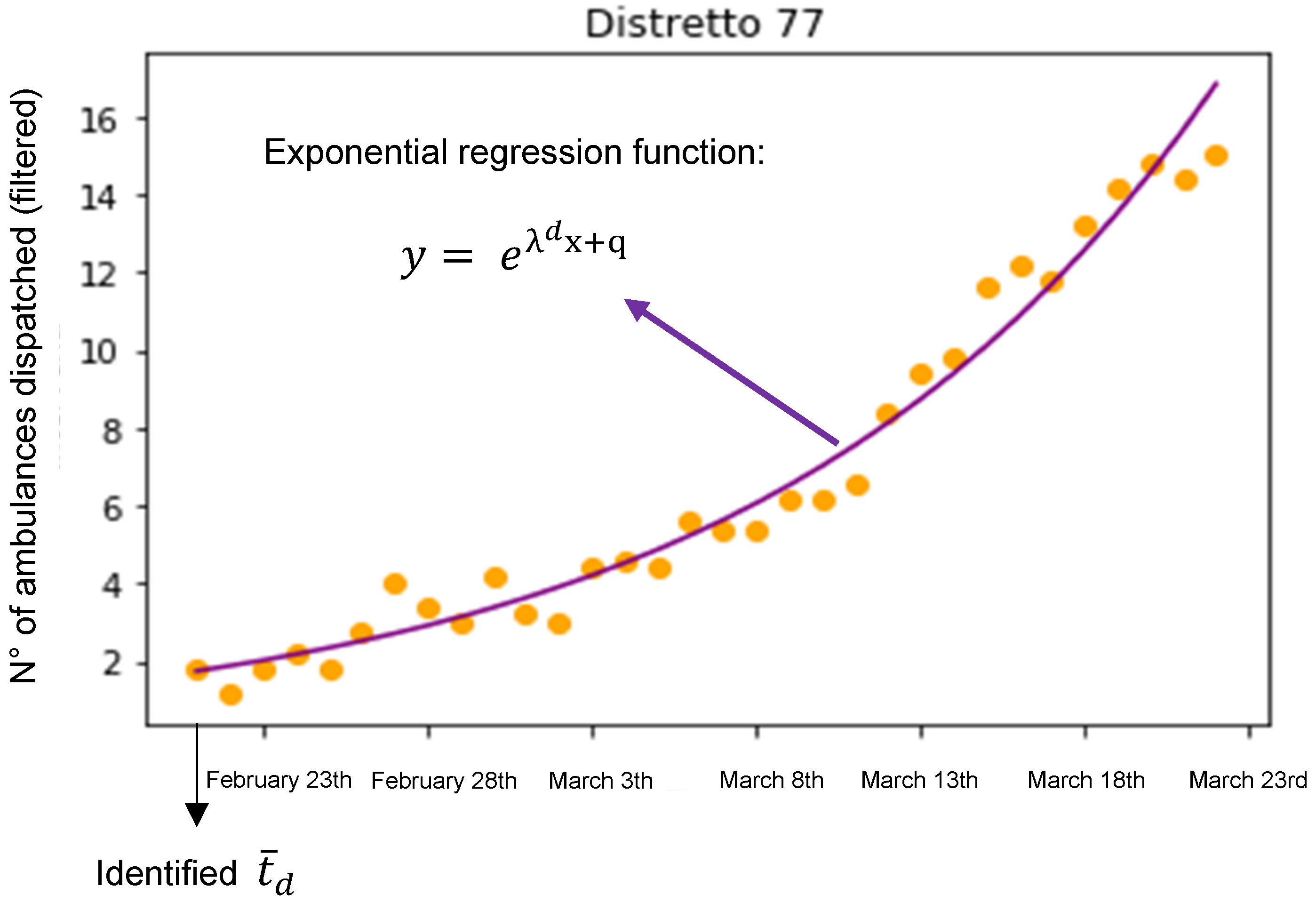
- A moving average filter with a window of 5 days was applied;
- The exponential data regression in the form was iteratively computed on a sequence having as its last point the value at 23 March 2020 (last data point available) and as the first point each possible previous day (moving backward up to 1 January 2020); then, the earliest point with a correlation coefficient R2 > 0.9 was selected as the starting day () of the pandemic diffusion;
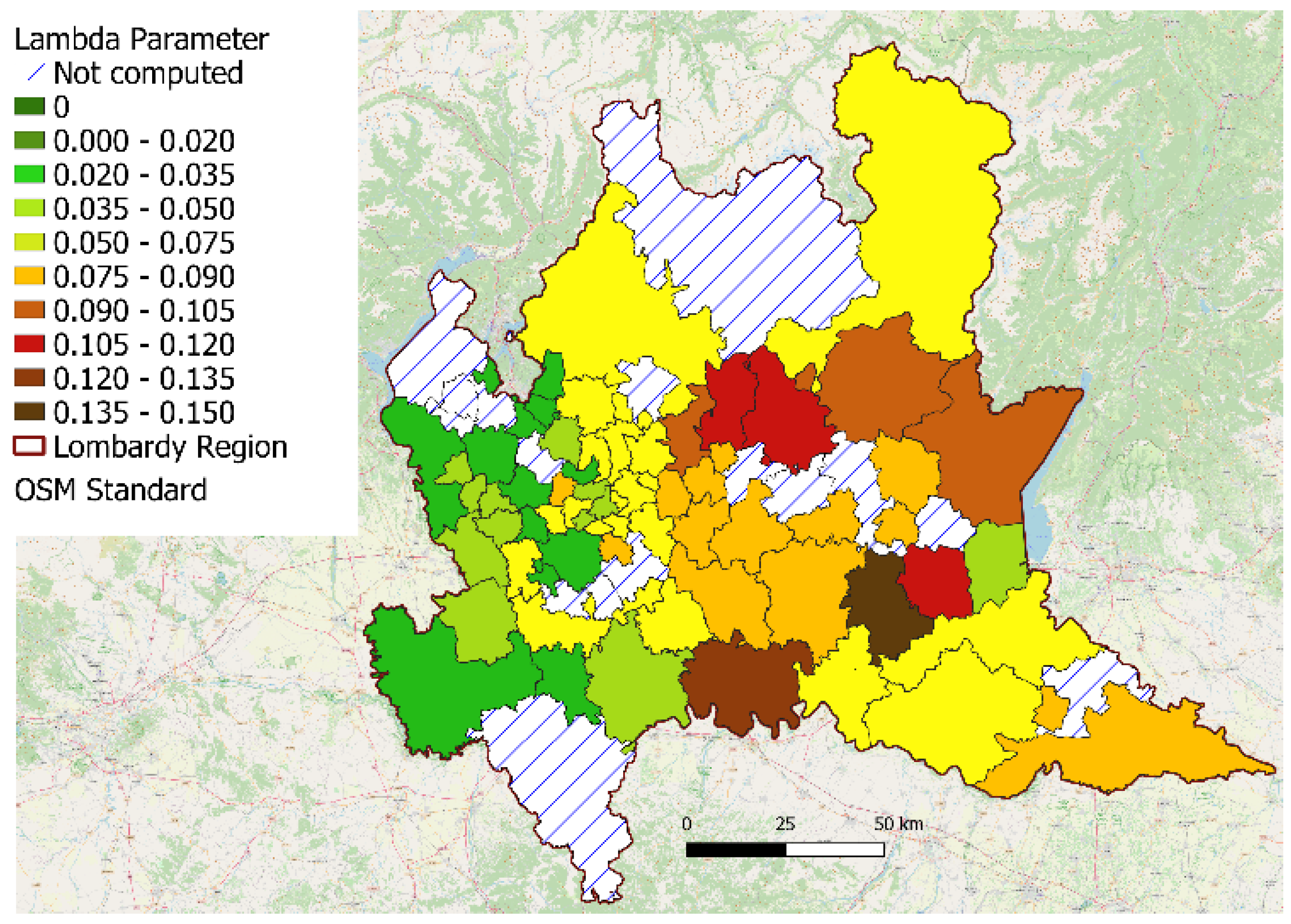
- The parameter resulting from the exponential regression between () and 23 March 2020 was considered as a representative estimate of the speed of the pandemic diffusion for the district d.
3. Results
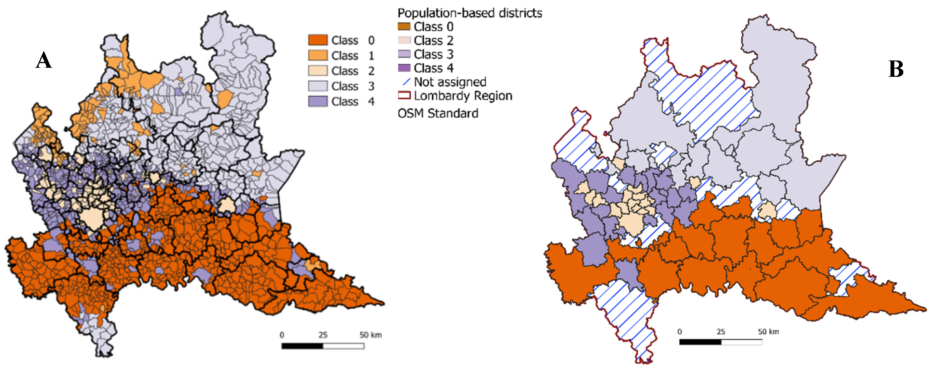
3.1. Territorial Subdivision and Clustering
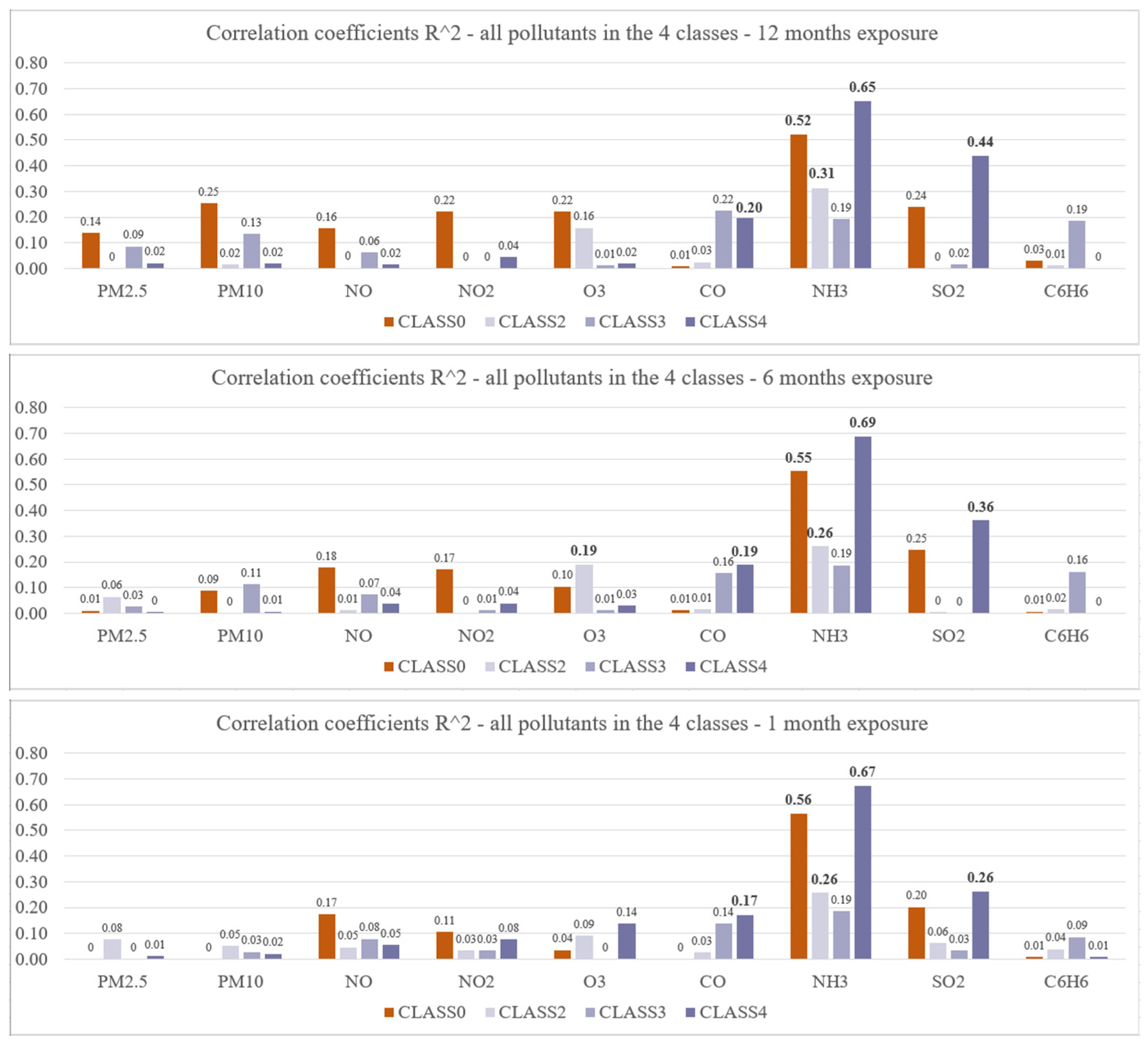
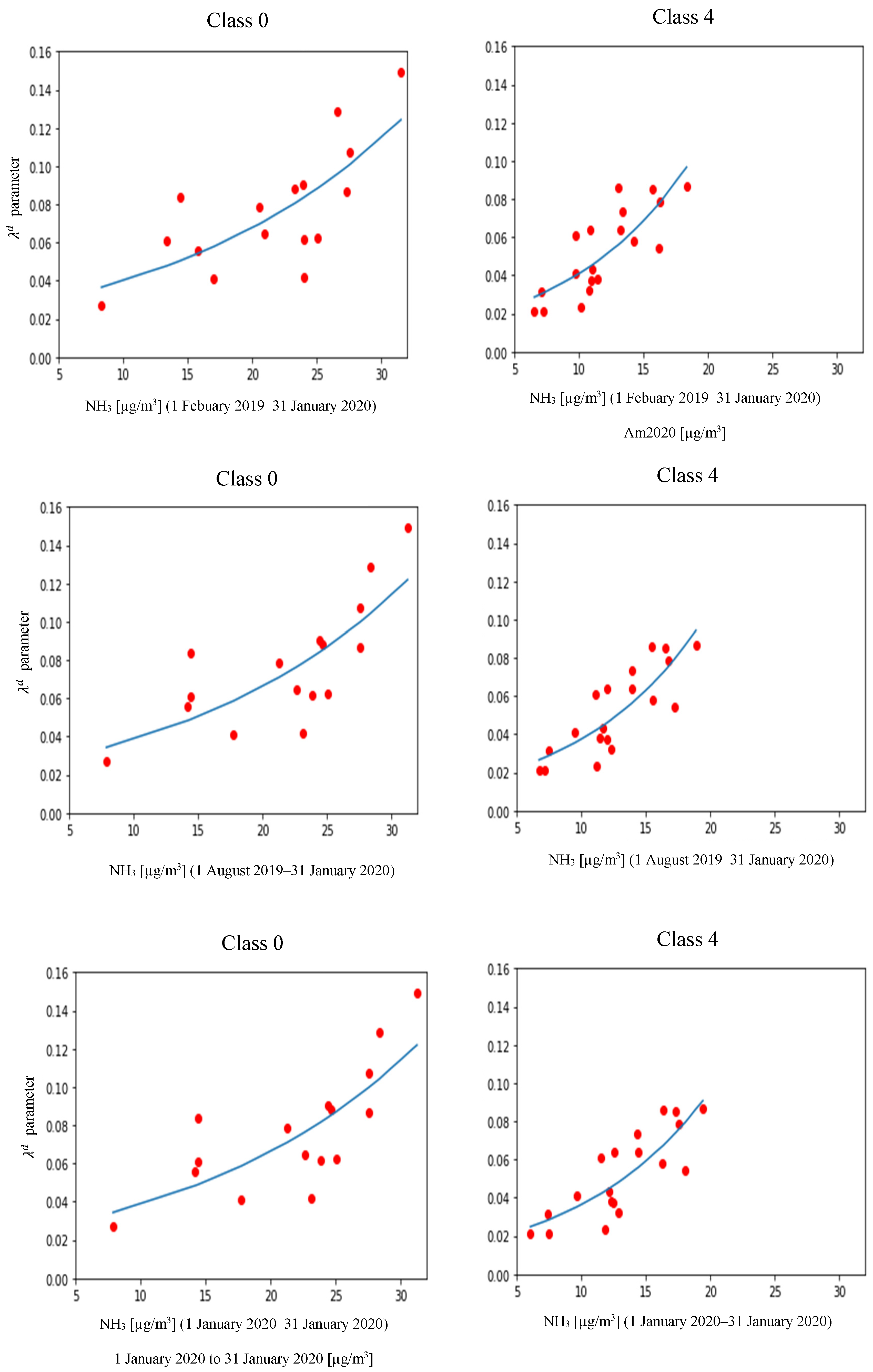
3.2. Data Correlations
4. Discussion
5. Conclusions
- The reliability of analyzed data, by considering the number of ambulances dispatches for respiratory issues;
- The management of confounding factors, by comparing only territories with similar land-use characteristics;
- Considering the time component, by focusing on the initial spread of the disease, to avoid biases introduced by effect of lockdown measures;
- The method to estimate the speed of diffusion, by computing the slope of the exponential interpolation of daily data rather than using cumulated data.
Author Contributions
Funding
Institutional Review Board Statement
Informed Consent Statement
Data Availability Statement
Conflicts of Interest
References
- Mallapaty, S. How deadly is the coronavirus? Scientists are close to an answer. Nat. Cell Biol. 2020, 582, 467–468. [Google Scholar] [CrossRef] [PubMed]
- Carugno, M.; Consonni, D.; Randi, G.; Catelan, D.; Grisotto, L.; Bertazzi, P.A.; Biggeri, A.; Baccini, M. Air pollution exposure, cause-specific deaths and hospitalizations in a highly polluted Italian region. Environ. Res. 2016, 147, 415–424. [Google Scholar] [CrossRef] [Green Version]
- Teoldi, F.; Lodi, M.; Benfenati, E.; Colombo, A.; Baderna, D. Air quality in the Olona Valley and in vitro human health effects. Sci. Total Environ. 2017, 579, 1929–1939. [Google Scholar] [CrossRef]
- Renzi, M.; Forastiere, F.; Schwartz, J.; Davoli, M.; Michelozzi, P.; Stafoggia, M. Long-Term PM10 Exposure and Cause-Specific Mortality in the Latium Region (Italy): A Difference-in-Differences Approach. Environ. Health Perspect. 2019, 127, 67004. [Google Scholar] [CrossRef]
- De Marco, A.; Proietti, C.; Anav, A.; Ciancarella, L.; D’Elia, I.; Fares, S.; Fornasier, M.F.; Fusaro, L.; Gualtieri, M.; Manes, F.; et al. Impacts of air pollution on human and ecosystem health, and implications for the National Emission Ceilings Directive: Insights from Italy. Environ. Int. 2019, 125, 320–333. [Google Scholar] [CrossRef]
- Frontera, A.; Martin, C.; Vlachos, K.; Sgubin, G. Regional air pollution persistence links to COVID-19 infection zoning. J. Infect. 2020, 81, 318–356. [Google Scholar] [CrossRef]
- Domingo, J.L.; Rovira, J. Effects of air pollutants on the transmission and severity of respiratory viral infections. Environ. Res. 2020, 187, 109650. [Google Scholar] [CrossRef]
- Bashir, M.F.; Jiang, B.; Komal, B.; Bashir, M.A.; Farooq, T.H.; Iqbal, N.; Bashir, M. Correlation between environmental pollution indicators and COVID-19 pandemic: A brief study in Californian context. Environ. Res. 2020, 187, 109652. [Google Scholar] [CrossRef]
- Chau, T.T.; Wang, K.Y. An association between air pollution and daily most frequently visits of eighteen outpatient diseases in an industrial city. Nat. Sci. Rep. 2020, 10, 2321. [Google Scholar] [CrossRef] [PubMed] [Green Version]
- Bontempi, E. First data analysis about possible COVID-19 virus airborne diffusion due to air particulate matter (PM): The case of Lombardy (Italy). Environ. Res. 2020, 186, 109639. [Google Scholar] [CrossRef]
- Coccia, M. Factors determining the diffusion of COVID-19 and suggested strategy to prevent future accelerated viral infectivity similar to COVID. Sci. Total Environ. 2020, 729, 138474. [Google Scholar] [CrossRef]
- Fattorini, D.; Regoli, F. Role of the chronic air pollution levels in the COVID-19 outbreak risk in Italy. Environ. Pollut. 2020, 264, 114732. [Google Scholar] [CrossRef]
- Fiasca, F.; Minelli, M.; Maio, D.; Minelli, M.; Vergallo, I.; Necozione, S.; Mattei, A. Associations between COVID-19 Incidence Rates and the Exposure to PM2.5 and NO2: A Nationwide Observational Study in Italy. Int. J. Environ. Res. Public Health 2020, 17, 9318. [Google Scholar] [CrossRef] [PubMed]
- Frontera, A.; Cianfanelli, L.; Vlachos, K.; Landoni, G.; Cremona, G. Severe air pollution links to higher mortality in COVID-19 patients: The “double-hit” hypothesis. J. Infect. 2020, 81, 255–259. [Google Scholar] [CrossRef] [PubMed]
- Martelletti, L.; Martelletti, P. Air Pollution and the Novel COVID-19 Disease: A Putative Disease Risk Factor. SN Compr. Clin. Med. 2020, 2, 383–387. [Google Scholar] [CrossRef] [Green Version]
- Sebastianelli, A.; Mauro, F.; Di Cosmo, G.; Passarini, F.; Carminati, M.; Ullo, S.L. AIRSENSE-TO-ACT: A Concept Paper for COVID-19 Countermeasures Based on Artificial Intelligence Algorithms and Multi-Source Data Processing. ISPRS Int. J. Geo-Inf. 2021, 10, 34. [Google Scholar] [CrossRef]
- Setti, L.; Passarini, F.; De Gennaro, G.; Barbieri, P.; Licen, S.; Perrone, M.G.; Piazzalunga, A.; Borelli, M.; Palmisani, J.; Di Gilio, A.; et al. Potential role of particulate matter in the spreading of COVID-19 in Northern Italy: First observational study based on initial epidemic diffusion. BMJ Open 2020, 10, e039338. [Google Scholar] [CrossRef]
- Zoran, M.A.; Savastru, R.S.; Savastru, D.M.; Tautan, M.N. Assessing the relationship between surface levels of PM2.5 and PM10 particulate matter impact on COVID-19 in Milan, Italy. Sci. Total. Environ. 2020, 738, 139825. [Google Scholar] [CrossRef]
- Zoran, M.A.; Savastru, R.S.; Savastru, D.M.; Tautan, M.N. Assessing the relationship between ground levels of ozone (O3) and nitrogen dioxide (NO2) with coronavirus (COVID-19) in Milan, Italy. Sci. Total. Environ. 2020, 740, 140005. [Google Scholar] [CrossRef]
- Liang, D.; Shi, L.; Zhao, J.; Liu, P.; Sarnat, J.A.; Gao, S.; Schwartz, J.; Liu, Y.; Ebelt, S.T.; Scovronick, N.; et al. Urban Air Pollution May Enhance COVID-19 Case-Fatality and Mortality Rates in the United States. Innovation 2020, 1, 100047. [Google Scholar] [CrossRef]
- Wu, X.; Nethery, R.C.; Sabath, M.B.; Braun, D.; Dominici, F. Air pollution and COVID-19 mortality in the United States: Strengths and limitations of an ecological regression analysis. Sci. Adv. 2020, 6, eabd4049. [Google Scholar] [CrossRef]
- Li, H.; Xu, X.L.; Dai, D.W.; Huang, Z.Y.; Ma, Z.; Guan, Y.J. Air pollution and temperature are associated with increased COVID-19 incidence: A time series study. Int. J. Infect. Dis. 2020, 97, 278–282. [Google Scholar] [CrossRef]
- Yao, Y.; Pan, J.; Wang, W.; Liu, Z.; Kan, H.; Qiu, Y.; Meng, X.; Wang, W. Association of particulate matter pollution and case fatality rate of COVID-19 in 49 Chinese cities. Sci. Total Environ. 2020, 741, 140396. [Google Scholar] [CrossRef]
- Zhu, Y.; Xie, J.; Huang, F.; Cao, L. Association between short-term exposure to air pollution and COVID-19 infection: Evidence from China. Sci. Total Environ. 2020, 727, 138704. [Google Scholar] [CrossRef]
- Magazzino, C.; Mele, M.; Schneider, N. The relationship between air pollution and COVID-19-related deaths: An application to three French cities. Appl. Energy 2020, 279, 115835. [Google Scholar] [CrossRef] [PubMed]
- Travaglio, M.; Yu, Y.; Popovic, R.; Selley, L.; Leal, N.S.; Martins, L.M. Links between air pollution and COVID-19 in England. Environ. Pollut. 2021, 268, 115859. [Google Scholar] [CrossRef] [PubMed]
- Ogen, Y. Assessing nitrogen dioxide (NO2) levels as a contributing factor to coronavirus (COVID-19) fatality. Sci. Total. Environ. 2020, 726, 138605. [Google Scholar] [CrossRef]
- Pansini, R.; Fornacca, D. Early Spread of COVID-19 in the Air-Polluted Regions of Eight Severely Affected Countries. Atmosphere 2021, 12, 795. [Google Scholar] [CrossRef]
- Contini, D.; Costabile, F. Does Air Pollution Influence COVID-19 Outbreaks? Atmosphere 2020, 11, 377. [Google Scholar] [CrossRef] [Green Version]
- Baud, D.; Qi, X.; Nielsen-Saines, K.; Musso, D.; Pomar, L.; Favre, G. Real estimates of mortality following COVID-19 infection. Lancet Infect. Dis. 2020, 20, 773. [Google Scholar] [CrossRef] [Green Version]
- Tuite, A.R.; Ng, V.; Rees, E.; Fisman, D. Estimation of COVID-19 outbreak size in Italy. Lancet Infect. Dis. 2020, 20, 537. [Google Scholar] [CrossRef] [Green Version]
- Istituto Superiore di Sanità, Roma–Aggiornamento Nazionale 09 Marzo 2020. Available online: https://www.ansa.it/documents/1583864041148_Bollettino.pdf (accessed on 19 July 2020).
- Gatto, M.; Bertuzzo, E.; Mari, L.; Miccoli, S.; Carraro, L.; Casagrandi, R.; Rinaldo, A. Spread and dynamics of the COVID-19 epidemic in Italy: Effects of emergency containment measures. Proc. Natl. Acad. Sci. USA 2020, 117, 10484–10491. [Google Scholar] [CrossRef] [Green Version]
- Giordano, G.; Blanchini, F.; Bruno, R.; Colaneri, P.; Di Filippo, A.; Di Matteo, A.; Colaneri, M. Modelling the COVID-19 epidemic and implementation of population-wide interventions in Italy. Nat. Med. 2020, 26, 855–860. [Google Scholar] [CrossRef]
- Riccò, M.; Ranzieri, S.; Balzarini, F.; Bragazzi, N.L.; Corradi, M. SARS-CoV-2 infection and air pollutants: Correlation or causation? Sci. Total Environ. 2020, 734, 139489. [Google Scholar] [CrossRef]
- Gianquintieri, L.; Brovelli, M.A.; Pagliosa, A.; Dassi, G.; Brambilla, P.M.; Bonora, R.; Sechi, G.M.; Caiani, E.G. Mapping Spatiotemporal Diffusion of COVID-19 in Lombardy (Italy) on the Base of Emergency Medical Services Activities. ISPRS Int. J. Geo-Inf. 2020, 9, 639. [Google Scholar] [CrossRef]
- Open Geospatial Consortium. Glossary of Terms. Available online: https://www.opengeospatial.org/ogc/glossary/g (accessed on 19 July 2020).
- Wu, Y.; Gu, B.; Erisman, J.W.; Reis, S.; Fang, Y.; Lu, X.; Zhang, X. PM2.5 pollution is substantially affected by ammonia emissions in China. Environ. Pollut. 2016, 218, 86–94. [Google Scholar] [CrossRef] [Green Version]
- Erisman, J.W.; Schaap, M. The need for ammonia abatement with respect to secondary PM reductions in Europe. Environ. Pollut. 2004, 129, 159–163. [Google Scholar] [CrossRef] [PubMed]
- Sapek, A. Ammonia Emissions from Non-Agricultural Sources. Pol. J. Environ. Stud. 2013, 22, 63–70. [Google Scholar]
- Bai, Z.; Dong, Y.; Wang, Z.; Zhu, T. Emission of ammonia from indoor concrete wall and assessment of human exposure. Environ. Int. 2006, 32, 303–311. [Google Scholar] [CrossRef] [PubMed]
- Loftus, C.; Yost, M.; Sampson, P.; Torres, E.; Arias, G.; Breckwich Vasquez, V.; Hartin, K.; Armstrong, J.; Tchong-French, M.; Vedal, S.; et al. Ambient Ammonia Exposures in an Agricultural Community and Pediatric Asthma Morbidity. Epidemiology 2015, 26, 794–801. [Google Scholar] [CrossRef]
- Neghab, M.; Mirzaei, A.; Kargar Shouroki, F.; Jahangiri, M.; Zare, M.; Yousefinejad, S. Ventilatory disorders associated with occupational inhalation exposure to nitrogen trihydride (ammonia). Ind. Health 2018, 56, 427–435. [Google Scholar] [CrossRef] [PubMed] [Green Version]
- Julin, J.; Murphy, B.N.; Patoulias, D.; Fountoukis, C.; Olenius, T.; Pandis, S.N.; Riipinen, I. Impacts of future european emission reductions on aerosol particle number concentrations accounting for effects of ammonia, amines, and organic species. Environ. Sci. Technol. 2018, 52, 692–700. [Google Scholar] [CrossRef]
- Blanes-Vidal, V.; Guàrdia, M.; Dai, X.R.; Nadimi, E.S. Emissions of NH3, CO2 and H2S during swine wastewater management: Characterization of transient emissions after air-liquid interface disturbances. Environ. Geochem. Health 2012, 54, 408–418. [Google Scholar] [CrossRef]
- Higashiyama, H.; Yoshimoto, D.; Okamoto, Y.; Kikkawa, H.; Asano, S.; Kinoshita, M. Receptor-activated Smad localisation in Bleomycin-induced pulmonary fibrosis. J. Clin. Pathol. 2007, 60, 283–289. [Google Scholar] [CrossRef] [PubMed] [Green Version]
- Coltart, I.; Tranah, T.H.; Shawcross, D.L. Inflammation and hepatic encephalopathy. Arch. Biochem. Biophys. 2013, 536, 189–196. [Google Scholar] [CrossRef] [PubMed]
- Nordmeier, F.; Doerr, A.; Laschke, M.W.; Menger, M.D.; Schmidt, P.H.; Schaefer, N.; Meyer, M.R. Are pigs a suitable animal model for in vivo metabolism studies of new psychoactive substances? A comparison study using different in vitro/in vivo tools and U-47700 as model drug. Toxicol. Lett. 2020, 319, 12–19. [Google Scholar] [CrossRef]
- Wang, H.; Zeng, X.; Zhang, X.; Liu, H.; Xing, H. Ammonia exposure induces oxidative stress and inflammation by destroying the microtubule structures and the balance of solute carriers in the trachea of pigs. Ecotoxicol. Environ. Saf. 2021, 212, 111974. [Google Scholar] [CrossRef] [PubMed]
- Durackova, Z. Some current insights into oxidative stress. Physiol. Res. 2010, 59, 459–469. [Google Scholar] [CrossRef]
- McCullough, L.E.; Santella, R.M.; Cleveland, R.J.; Bradshaw, P.T.; Millikan, R.C.; North, K.E.; Olshan, A.F.; Eng, S.M.; Ambrosone, C.B.; Ahn, J.; et al. Polymorphisms in oxidative stress genes, physical activity, and breast cancer risk. Cancer Causes Control 2012, 23, 1949–1958. [Google Scholar] [CrossRef] [Green Version]
- Hegazi, M.M.; Attia, Z.I.; Ashour, O.A. Oxidative stress and antioxidant enzymes in liver and white muscle of Nile tilapia juveniles in chronic ammonia exposure. Aquat. Toxicol. 2010, 99, 118–125. [Google Scholar] [CrossRef]
- Zhang, J.; Li, C.; Tang, X.; Lu, Q.; Sa, R.; Zhang, H. High concentrations of atmospheric ammonia induce alterations in the hepatic proteome of broilers (Gallus gallus): An iTRAQ-based quantitative proteomic analysis. PLoS ONE 2015, 10, e0123596. [Google Scholar] [CrossRef] [Green Version]
- Cecchini, R.; Cecchini, A.L. SARS-CoV-2 infection pathogenesis is related to oxidative stress as a response to aggression. Med. Hypotheses 2020, 143, 110102. [Google Scholar] [CrossRef]
- Chernyak, B.V.; Popova, E.N.; Prikhodko, A.S.; Grebenchikov, O.A.; Zinovkina, L.A.; Zinovkin, R.A. COVID-19 and Oxidative Stress. Biochemistry 2020, 85, 1543–1553. [Google Scholar] [CrossRef]
- Gjyshi, O.; Bottero, V.; Veettil, M.V. Kaposi’s sarcoma-associated herpesvirus induces Nrf 2 during de novo infection of endothelial cells to create a microenvironment conducive to infection. PLoS Pathog. 2014, 10, e1004460. [Google Scholar] [CrossRef]
- Hadei, M.; Hopke, P.K.; Jonidi, A.; Shahsavani, A. A Letter about the Airborne Transmission of SARS-CoV-2 Based on the Current Evidence. Aerosol Air Qual. Res. 2020, 20, 911–914. [Google Scholar] [CrossRef] [Green Version]
- Liu, Y.; Ning, Z.; Chen, Y.; Guo, M.; Liu, Y.; Gali, N.K.; Sun, L.; Duan, Y.; Cai, J.; Westerdahl, D.; et al. Aerodynamic analysis of SARS-CoV-2 in two Wuhan hospitals. Nature 2020, 582, 557–560. [Google Scholar] [CrossRef] [PubMed]
- Ma, Q.; Qi, Y.; Shan, Q.; Liu, S.; He, H. Understanding the knowledge gaps between air pollution controls and health impacts including pathogen epidemic. Environ. Res. 2020, 189, 109949. [Google Scholar] [CrossRef]
- Morawska, L.; Milton, D.K. It Is Time to Address Airborne Transmission of Coronavirus Disease 2019 (COVID-19). Clin. Infect. Dis. 2020, 71, 2311–2313. [Google Scholar] [CrossRef] [PubMed]
- Qu, G.; Li, X.; Hu, L.; Jiang, G. An Imperative Need for Research on the Role of Environmental Factors in Transmission of Novel Coronavirus (COVID-19). Environ. Sci. Technol. 2020, 54, 3730–3732. [Google Scholar] [CrossRef]
- Setti, L.; Passarini, F.; De Gennaro, G.; Barbieri, P.; Perrone, M.G.; Borelli, M.; Palmisani, J.; Di Gilio, A.; Piscitelli, P.; Miani, A. Airborne Transmission Route of COVID-19: Why 2 Meters/6 Feet of Inter-Personal Distance Could Not Be Enough. Int. J. Environ. Res. Public Health 2020, 17, 2932. [Google Scholar] [CrossRef] [Green Version]
- Belosi, F.; Conte, M.; Gianelle, V.; Santachiara, G.; Contini, D. On the concentration of SARS-CoV-2 in outdoor air and the interaction with pre-existing atmospheric particles. Environ. Res. 2021, 193, 110603. [Google Scholar] [CrossRef] [PubMed]
- Cao, C.; Jiang, W.; Wang, B.; Fang, J.; Lang, J.; Tian, G.; Jiang, J.; Zhu, T.F. Inhalable Microorganisms in Beijing’s PM2.5 and PM10 Pollutants during a Severe Smog Event. Environ. Sci. Technol. 2014, 48, 1499–1507. [Google Scholar] [CrossRef] [PubMed]
- Liang, Y.; Fang, L.; Pan, H.; Zhang, K.; Kan, H.; Brook, J.R.; Sun, Q. PM2.5 in Beijing–Temporal pattern and its association with influenza. Environ. Health 2014, 13, 1–8. [Google Scholar] [CrossRef] [Green Version]
- Setti, L.; Passarini, F.; De Gennaro, G.; Barbieri, P.; Pallavicini, A.; Ruscio, M.; Piscitelli, P.; Colao, A.; Miani, A. Searching for SARS-CoV-2 on Particulate Matter: A Possible Early Indicator of COVID-19 Epidemic Recurrence. Int. J. Environ. Res. Public Health 2020, 17, 2986. [Google Scholar] [CrossRef]
- Setti, L.; Passarini, F.; De Gennaro, G.; Barbieri, P.; Perrone, M.G.; Borelli, M.; Palmisani, J.; Di Gilio, A.; Torboli, A.; Fontana, F.; et al. SARS-CoV-2RNA found on particulate matter of Bergamo in Northern Italy: First evidence. Environ. Res. 2020, 188, 109754. [Google Scholar] [CrossRef] [PubMed]
- Conticini, E.; Frediani, B.; Caro, D. Can atmospheric pollution be considered a co-factor in extremely high level of SARS-CoV-2 lethality in Northern Italy? Environ. Pollut. 2020, 261, 114465. [Google Scholar] [CrossRef]


| TC Number | % Urbanized Area | % Industrial Area | % Agricultural Area | % Natural Area | Mean Tax Contribution (€) |
|---|---|---|---|---|---|
| 0 | 7.97 | 4.6 | 76.28 | 11.21 | 15,332.84 |
| 1 | 8.47 | 1.23 | 3.51 | 86.76 | 10,589.85 |
| 2 | 45.05 | 16.9 | 17.02 | 20.99 | 18,124.67 |
| 3 | 6.46 | 1.52 | 2.84 | 89.12 | 15,513.17 |
| 4 | 23.21 | 10.53 | 33.18 | 33.13 | 17,714.22 |
| Class 0 | Class 2 | Class 3 | Class 4 | ||
|---|---|---|---|---|---|
| Ambulances dispatched/100k residents (1 January 2020–23 March 2020) | Total distribution in districts | 699.6 664.8 (561.1–778.1) | 437.5 394.7 (340.9–473.4) | 650.1 587.7 (469.9–737) | 430.7 393 (341.1–503.3) |
| PM2.5 [µg/m3] | 12 months 6 months 1 month | 18 (11–31) 21 (13–35) 51 (36–64) | 17 (11–28) 18 (12–32) 48 (35–62) | 14 (7–24) 12 (5–24) 22 (4–39.25) | 16 (11–27) 17 (11–30) 44 (33–57) |
| PM10 [µg/m3] | 12 months 6 months 1 month | 27 (18–42) 29 (20–46) 62 (47–77.5) | 24 (17–35) 26 (17–41) 59 (44–75) | 19 (11–30) 20 (10–30) 34 (18.5–52) | 24 (17–37) 25 (17–40) 57 (42–72) |
| NO [µg/m3] | 12 months 6 months 1 month | 26 (14–52) 32 (16–65) 80 (53–117) | 53 (29–104) 68 (34–131) 164 (101–256) | 20 (11–41) 25 (13–53) 59 (29–98) | 31 (17–64) 39 (20–84) 114 (66–185) |
| NO2 [µg/m3] | 12 months 6 months 1 month | 20 (11–33) 23 (13–35) 39 (31–48) | 37 (22–56) 40 (24–58) 64 (49–80) | 16 (9–29) 19 (10–32) 36 (22–50) | 23 (13–39) 27 (15–41) 48 (36–64) |
| O3 [µg/m3] | 12 months 6 months 1 month | 39 (10–74) 20 (4–50) 4 (2–10) | 40 (8–75) 18 (6–53) 6 (5–10) | 58 (26–87) 38 (13–69) 21 (7–54) | 40 (10–74) 19 (6–51) 6 (3–11) |
| CO [mg/m3] | 12 months 6 months 1 month | 0.3 (0.2–0.6) 0.5 (0.3–0.7) 0.9 (0.7–1.1) | 0.6 (0.3–0.9) 0.7 (0.4–1) 1.2 (0.8–1.6) | 0.3 (0.2–0.4) 0.3 (0.2–0.4) 0.4 (0.2–0.6) | 0.4 (0.3–0.7) 0.5 (0.3–0.8) 1 (0.7–1.3) |
| NH3 [µg/m3] | 12 months 6 months 1 month | 17 (7–40) 17 (6–37) 22 (6–43) | 13 (6–18) 14 (12–16) 15 (13–16) | 3 (1–6) 3 (0–5) 2 (0–7) | 4 (2–8) 3 (2–7) 3 (2–5) |
| SO2 [µg/m3] | 12 months 6 months 1 month | 2.9 (1.7–4.1) 2.8 (1.7–4) 2.9 (1.9–3.8) | 2.2 (1.3–3.5) 2.5 (1.5–3.8) 3.6 (1.9–6) | 1.1 (0.7–1.9) 1.5 (0.9–2.4) 2.5 (1.6–3.6) | 2 (1.2–3) 2.3 (1.5–3.2) 3 (2.3–4) |
| C6H6 [µg/m3] | 12 months 6 months 1 month | 0.4 (0.2–0.8) 0.5 (0.3–1.3) 2 (1.6–2.5) | 0.9 (0.5–1.5) 1.1 (0.6–1.9) 2.4 (1.5–3.7) | 0.5 (0.3–1.5) 0.9 (0.3–2.1) 1.9 (1.4–2.7) | 0.4 (0.2–0.9) 0.5 (0.3–1) 1.6 (1.2–2.2) |
| Territorial Class | Exposure Time Period [Months] | R2 Exp Regression | |
|---|---|---|---|
| Class 4 | 12 | 0.0943 | 0.652 |
| Class 4 | 6 | 0.0968 | 0.688 |
| Class 4 | 1 | 0.0922 | 0.674 |
| Class 0 | 12 | 0.0596 | 0.523 |
| Class 0 | 6 | 0.067 | 0.553 |
| Class 0 | 1 | 0.0643 | 0.565 |
Publisher’s Note: MDPI stays neutral with regard to jurisdictional claims in published maps and institutional affiliations. |
© 2021 by the authors. Licensee MDPI, Basel, Switzerland. This article is an open access article distributed under the terms and conditions of the Creative Commons Attribution (CC BY) license (https://creativecommons.org/licenses/by/4.0/).
Share and Cite
Gianquintieri, L.; Brovelli, M.A.; Pagliosa, A.; Bonora, R.; Sechi, G.M.; Caiani, E.G. Geospatial Correlation Analysis between Air Pollution Indicators and Estimated Speed of COVID-19 Diffusion in the Lombardy Region (Italy). Int. J. Environ. Res. Public Health 2021, 18, 12154. https://doi.org/10.3390/ijerph182212154
Gianquintieri L, Brovelli MA, Pagliosa A, Bonora R, Sechi GM, Caiani EG. Geospatial Correlation Analysis between Air Pollution Indicators and Estimated Speed of COVID-19 Diffusion in the Lombardy Region (Italy). International Journal of Environmental Research and Public Health. 2021; 18(22):12154. https://doi.org/10.3390/ijerph182212154
Chicago/Turabian StyleGianquintieri, Lorenzo, Maria Antonia Brovelli, Andrea Pagliosa, Rodolfo Bonora, Giuseppe Maria Sechi, and Enrico Gianluca Caiani. 2021. "Geospatial Correlation Analysis between Air Pollution Indicators and Estimated Speed of COVID-19 Diffusion in the Lombardy Region (Italy)" International Journal of Environmental Research and Public Health 18, no. 22: 12154. https://doi.org/10.3390/ijerph182212154
APA StyleGianquintieri, L., Brovelli, M. A., Pagliosa, A., Bonora, R., Sechi, G. M., & Caiani, E. G. (2021). Geospatial Correlation Analysis between Air Pollution Indicators and Estimated Speed of COVID-19 Diffusion in the Lombardy Region (Italy). International Journal of Environmental Research and Public Health, 18(22), 12154. https://doi.org/10.3390/ijerph182212154