Article

Applying a Complex Integrated Method for Mapping and Assessment of the Degraded Ecosystem Hotspots from Romania

1
National Institute for Economic Research “Costin C. Kiriţescu” (INCE), Romanian Academy, 13 September Street No. 13, 050711 Bucharest, Romania
2
Department of Geography, University of Craiova, Al. I. Cuza Street No. 13, 200585 Craiova, Romania
3
Remote Sensing and Satellite Meteorology Laboratory, National Meteorological Administration, 013686 Bucharest, Romania
4
National Institute of Research and Development for Biological Sciences, Spl. Independentei No. 296, 060031 Bucharest, Romania
5
Institute of Research for Agriculture Economy and Rural Development, Bd. Marasti No. 61, 011464 Bucharest, Romania
6
Faculty of Geography, Babes-Bolyai University, 400006 Cluj-Napoca, Romania
*
Author to whom correspondence should be addressed.
Int. J. Environ. Res. Public Health 2021, 18(21), 11416; https://doi.org/10.3390/ijerph182111416
Submission received: 17 September 2021 / Revised: 22 October 2021 / Accepted: 25 October 2021 / Published: 29 October 2021

Abstract

:
To meet the global challenges of climate change and human activity pressure on biodiversity conservation, it has become vital to map such pressure hotspots. Large areas, such as nation-wide regions, are difficult to map from the point of view of the resources needed for such mapping (human resources, hard and soft resources). European biodiversity policies have focused on restoring degraded ecosystems by at least 10% by 2020, and new policies aim to restore up to 30% of degraded ecosystems by 2030. In this study, methods developed and applied for the assessment of the degradation state of the ecosystems in a semi-automatic manner for the entire Romanian territory (238,391 km2) are presented. The following ecosystems were analyzed: forestry, grassland, rivers, lakes, caves and coastal areas. The information and data covering all the ecoregions of the Romania (~110,000 km2) were analyzed and processed, based on GIS and remote sensing techniques. The largest degraded areas were identified within the coastal area (49.80%), grassland ecosystems (38.59%) and the cave ecosystems (2.66%), while 27.64% of rivers ecosystems were degraded, followed by 8.52% of forest ecosystems, and 14.05% of lakes ecosystems. This analysis can contribute to better definition of the locations of the most affected areas, which will yield a useful spatial representation for future ecological reconstruction strategy.

1. Introduction

The evaluation of the state of ecosystems, as the fundamental structural and functional unit of living matter, is a constant concern of global and European policies, in order to establish guidelines for preventing the loss of their functions. The assessment of the condition of ecosystems necessitates extensive analysis of their physical, chemical and biological quality at a particular moment and measurement of the impacts of major pressures that are arising. Natural ecosystems are constantly exposed to pressures from over-exploitation of resources, extensive hunting, climate change and pollution [1,2]. Some authors consider that the highest direct impact on an ecosystem’s state is represented by anthropogenic pressures (overharvesting and land use change) leading to biodiversity loss [3].
To accurately evaluate the ecosystem services provided by a particular area, first, the state of the ecosystem must be studied. The state of the ecosystem is the first level in the flow of services from nature to society [4], and it defines the ability of the ecosystem to provide services. Pressures from human activity, such as pollution or overuse, can have an impact on the state of the ecosystem, thus reducing its ability to provide services to society [5,6]. The good condition of ecosystems is not considered a service itself; however, it is indispensable as it is an essential condition for human activity.
The ecosystem is degraded when the viability of natural processes and relationships within it are removed or disturbed by anthropogenic activity or the action of natural factors [7]. It is also a process with multiple effects on climate change, biodiversity changes and ecosystem services [8].
Europe is facing a continuing loss of biodiversity, and natural ecosystems are diminishing, especially wetlands, by about 50% [9]. As a member of the European Union (EU), Romania promotes and supports the protection of ecosystems, being part of the United Nations Convention on Biological Diversity (“Convention on Biological Diversity”, 1992). However, like most European countries, Romania is experiencing an increase in its share of degraded ecosystems [10,11].
The restoration of the geological environment and the affected terrestrial ecosystems involves bringing them as close as possible to their natural state, by applying complementary and compensatory cleaning, remediation and/or reconstruction measures and by eliminating any significant risk according to the category of land use. To do this it is necessary to properly evaluate their degradation state and the drivers of this degradation.
Changes in ecosystems are frequently identified on the basis of satellite imagery [12,13]. Most methods focus on biomass evaluation [14,15,16], leaf area index (LAI) [17] or productivity [18,19,20]. The Global Climate Observing System (GCOS), promotes LAI as an essential climate variable (ECV), being a key parameter used in woody ecosystems [21].
In many studies, the health of the ecosystem is analyzed based on GPP (gross primary production) or NPP (net primary production) indices and a vegetation index, such as the normalized-difference vegetation index (NDVI). The high value of these indices does not necessarily mean a good state of health [22], as it may be due to invasive species. In the same way, primary productivity is related not only to variations in CO2 in the atmosphere but also to climate change. Globally, productivity has increased in the last 20 years [23].
Machine learning algorithms such as Random Forest (RF) and Support Vector Machine (SVM) are used to identify and monitor vegetation types within forest [24] and grassland ecosystems [25]. Moreover, the SVM image classification method is useful in identifying invasive plant species [26,27], one of the important criteria in the evaluation of grassland ecosystems [27]. Some authors used satellite imagery (Sentinel 2, Landsat 8) and machine learning processes to locate forest treatments over large spatial extents [28].
Another recent analytical framework for the mapping and assessment of ecosystem condition [29] proposed indicators related to environmental pressures (physical and chemical quality) and ecosystem attributes (biological quality) based on a combination of individual metrics.
In October 2010, Japan and the EU member states at the Nagoya Biodiversity Summit signed the Convention on Biological Diversity. In order to achieve its EU biodiversity policy goals and to align with international commitments in the Convention on Biological Diversity, in May 2011, the EU adopted the Biodiversity Strategy to 2020. To achieve Target 2: “Maintain and restore ecosystems and their services”, i.e., the restoration of at least 15% of the degraded ecosystems by 2020, the document proposes that by 2014 each member state should develop a strategic framework for establishing the priorities for the restoration of ecosystems at a national level. In order to respond to the development needs and to contribute to the EU 2020 Strategy, in 2014, the Large Infrastructure Operational Program (LIOP) strategy was elaborated in Romania. Within LIOP, priority axis 4 was established for the promotion of ecological reconstruction projects [30]. Therefore, an assessment and mapping of Romanian degraded ecosystems was necessary. Given the need for composite indicators on ecosystem condition that can reflect the overall quality of an ecosystem asset in terms of its characteristics, the mapping and evaluating of degraded ecosystems in Romania were done.
The results of this paper are based on research started in April 2016, comprising detailed assessment for each type of ecosystem. The databases used were provided by various Romanian and European institutions. These were mainly spatial data, statistical data and satellite images. In the first phase, the degradation criteria and indicators for each type of ecosystem, the degradation classes and the sustainability thresholds were established, as well as the limits and the methodology for ecosystem mapping. In the second phase, the mapping and evaluation of the natural ecosystems were performed, as well as the validation of the results. The integration of all data was achieved and completed in May 2021.
EU Biodiversity Strategy to 2020 set objectives toward mapping and assessing the state of ecosystems from each member state. The target of this strategy was to restore 15% of degraded ecosystems [30] and the current EU-wide Biodiversity Strategy to 2030 aims to protect at least 30% of land and 30% of sea in Europe [31].
The main objectives of our study were as follows: to define and identify the types of natural and semi-natural ecosystems existing in Romania; to develop a nationally applicable methodology for the evaluation of each type of natural and semi-natural ecosystem; and, in this paper, to assess the complete ecosystem’s condition across Romanian territory in order to outline directions for their conservation status.

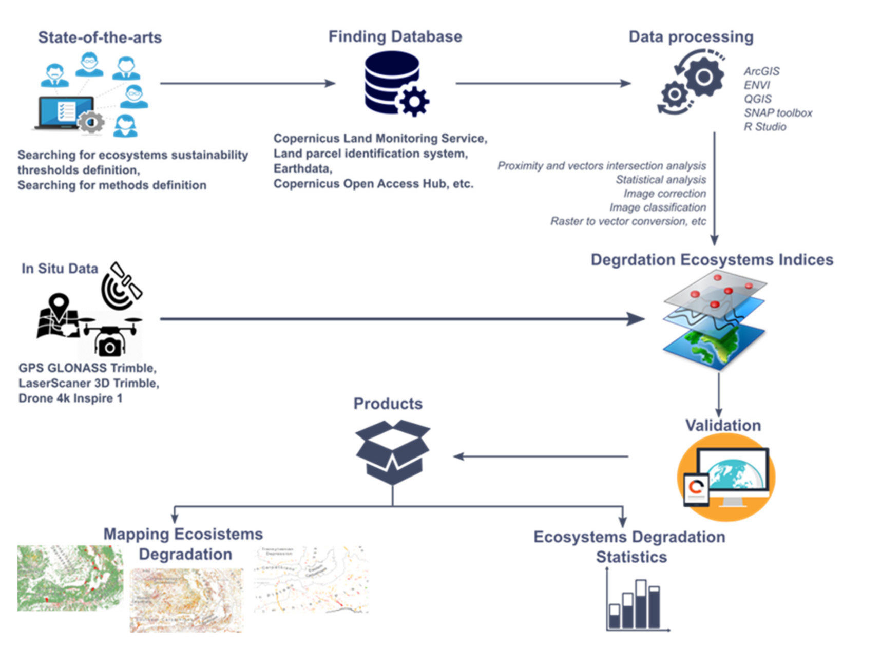
2. Materials and Methods
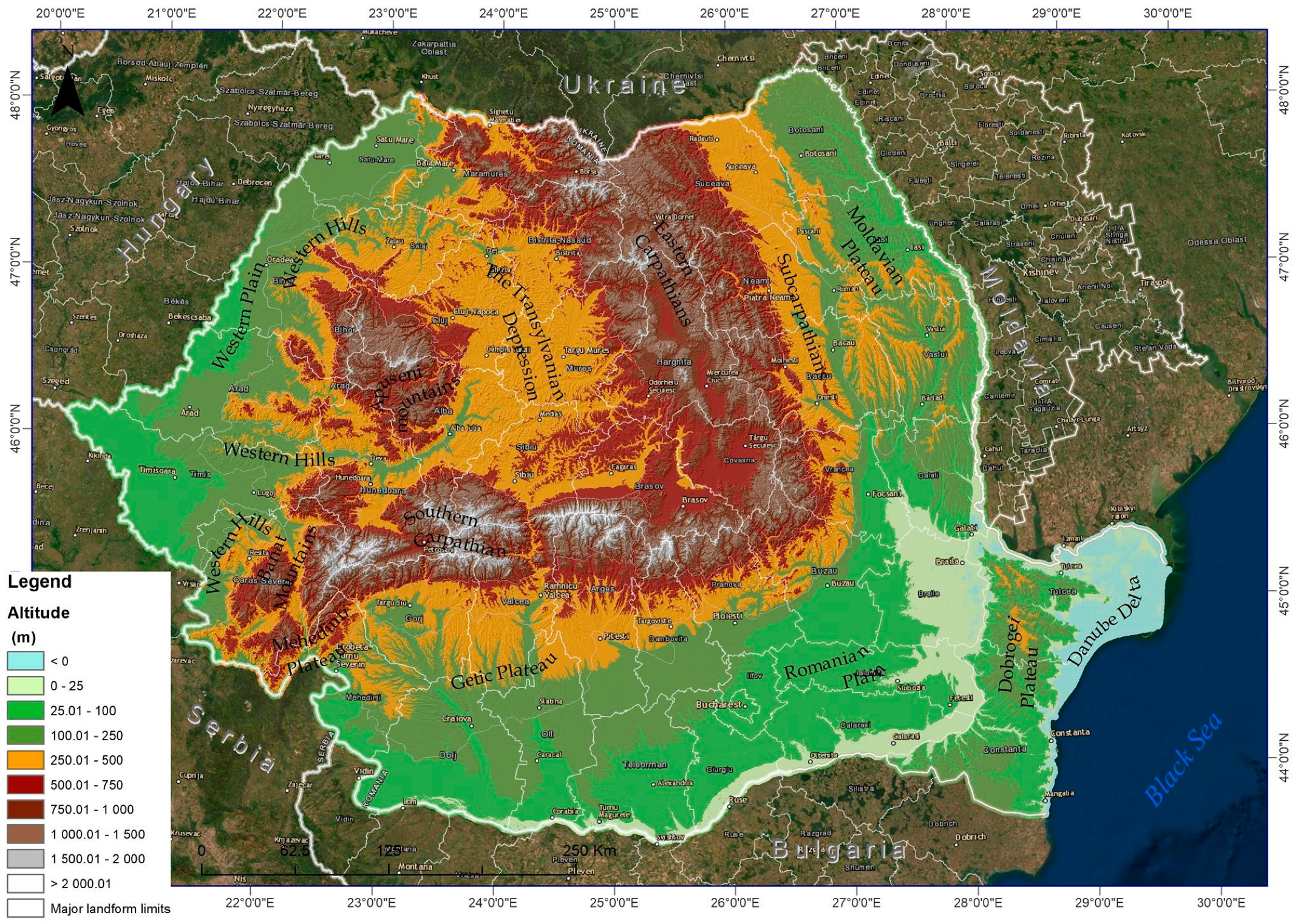
2.1. Study Area

Romania covers 238,391 km2 and is located in southeastern Europe, bordering on the Black Sea and the Danube. The major landforms are concentrically distributed [32], the Transylvanian depression in the center, surrounded by the Carpathian Mountains and hills. Two large plains surround the higher area, namely the Romanian Plain and the Western Plain, to which is added in SE the Danube Delta and Dobrogea Plateau (Figure 1). According to the Köppen–Geiger climate classification, Romania has a temperate continental climate [32]. From a bio-geographical point of view, in Romania, there are five biogeographical regions: Pannonian, Alpine, Continental, Steppic and Black Sea [33].
In a previous study, deliverable of the project Nature in public decisions—N4D, the following types of ecosystems were identified within the Romanian territory: terrestrial (woodland and forest, grassland, cave), freshwater (rivers and lakes), and marine (coastal). Forest ecosystems occupy a total area of about 71,890.84 km2, and about 32,357.14 km2 of Romanian area is grassland. There are also 339 caves. Rivers are 84,068.17 km in length, lakes represent 2248.28 km2, and 1574 km2 are coastal ecosystems [10,34].

2.2. Data Used

Due to the complexity of each ecosystem, a large number of data were used from different national and international sources available for the entire territory of Romania. Satellite images and satellite imagery products such as MODIS, Landsat and Sentinel 2 were used. Furthermore, vector data such as land use limits (CORINE Land Cover or Land parcel identification system), limits of territorial administrative units (TAUs), limits of protected natural areas, the hydrographic network, the road network, pollution sources, soil types, etc. and statistical data such as livestock and the number of inhabitants were used. The data sets used for each ecosystem are described in Table 1.

2.3. Methods

The workflow for the evaluation of the ecosystem’s condition (Figure 2) consisted in three phases. The first phase included state-of-the-art methods for identifying the potential pressures on each ecosystem; searching for ecosystem sustainability threshold definitions; identification of data sets available for the calculation of degradation indicators; data processing and analysis; validation of the applied method. For each ecosystem, a specific assessment methodology was involved. The second phase included correction and adjustment of each indicator used according to the field results; final data processing, field verification and validation. In the final stage, a topological attribute verification was performed.
The methodologies for establishing the level of degradation of the analyzed ecosystems included elements that have an impact on their health and sustainability. The determination of the level of degradation and the classes of degradation also took into account the capacity of ecosystems to support and provide ecosystem services in accordance with their basic functions (Supplementary Material).
The method describing the forest ecosystem’s status was based on the identification of deforested areas using the change detection algorithm between the land use category according to LPIS data [38,54] and the land use in the reference year of 2000, according to the tree canopy cover from Landsat [37]. The conservation status of forest ecosystems was established based on the VCF MODIS [37] product from 2000 to 2013 and the calculation of the linear trend for each pixel [10]. Forest degradation was analyzed by permanent changes in terms of land cover and land use. These changes reduce ecological integrity and health (SER, 2004) affecting the biodiversity and productivity of forests.
The evaluation of the grassland ecosystems was made based on six criteria, each criterion having a specific weight in the final result, Equation (1) [10]. The six criteria refer to the anthropo-zoogenic impact (proximity to localities, proximity to sheepfolds, the total livestock density) [55], stationary conditions (slope) and structural characteristics (invasive species and bare soil/erosions). Each criterion was divided into three classes of values, and each class received a score corresponding to the ecosystem condition, as follows: 0—natural, 1—semi-degraded, 2—degraded [10]. The identification of invasive species and soil or bare soil erosion was based on machine learning algorithms such as Random Forest (RF) and Support Vector Machine (SVM). The degradation state was assigned according to the value of the degradation index (DI). Thus, DI values between 0 and 30 indicated natural grassland ecosystems, between 35 and 60 they represented semi-degraded and between 65 and 180 degraded grassland ecosystems.
DI = (5 × C1) + (20 × C2) + (5 × C3) + (10 × C4) + (50 × C5) + (100 × C6)
where
C1 = proximity to localities (>4 km = natural, 2–4 km = semi-degraded, <2 km = degraded);
C2 = proximity to sheepfolds (>2 km = natural, 0.5–2 km = semi-degraded, <0.5 km = degraded);
C3 = slope (<15° = natural, 15°–30° = semi-degraded, >30° = degraded);
C4 = total livestock density (<±10% = natural, ±10–50% = semi-degraded, >±30% = degraded);
C5 = invasive species (<5% = natural, 5–20% = semi-degraded, >20% = degraded);
C6 = bare soil/erosions (<5% = natural, 5–20% = semi-degraded, >20% = degraded).
Cave ecosystems have been assessed on the basis of the Cave Conservation Index (CCI), which determines the impact of the cave environment and the threats and the vulnerability of the intrinsic characteristics of the caves [56]. CCI is calculated using the score obtained by completing the forms for establishing the impact on the environment of a cave, Rapid Assessment Protocol (RAP-cei) and the score obtained by completing the form to establish the vulnerability of a cave, in order to prioritize conservation and/or restoration actions [57]. Thus, for values between 0 and 34, the cave ecosystem was classified as natural, between 35 and 84 was semi-degraded, and over 85, it was classified as degraded [10].
River ecosystems were assessed based on 13 criteria, grouped into 4 major classes: A. Indicators of the human pressure on riparian areas (anthropization, vegetation cover, human settlements, sewage treatment plants, major pollution sources, transport network, natural protected areas), B. Indicators of substrate of the land adjacent to the watercourse (slope, soil permeability), C. Indicators associated with rivers (human interventions, ecological status of water bodies) and D. Indicators of the morphological complexity of water courses (sinuosity) [58]. Each indicator used in the multicriteria analysis was assigned a weight in the final analysis. The highest weights used in the multicriteria analysis for human pressure on riparian areas were as follows: the anthropization of the adjacent territory of a watercourse, vegetation cover in riparian areas, the presence of major pollution sources, the length of the transport network, human interventions in the riverbanks and the ecological status of water bodies [58].
The assessment of lake ecosystems was performed by combining the potential pollutant load (PPL) developed by [59], wastewater (W)–recreational (R)–agricultural (A)–size (S)–transportation (T)–industrial (I)–cover (C)–pollutant load (WRASTIC) [59] and lake vulnerability (LV) [60], resulting in a new index: WRASTIC-HI index [61,62]. This methodological stage included the analysis of a total of 3189 lakes and their classification by degradation classes.
The assessment of degradation status of the coastal ecosystem was made based on eight indicators, which can be grouped into biological indicators (related to the absence or presence of invasive species), hydro-morphological indicators (related to the presence of wastewater treatment plants, the presence of demographic aggregation poles, shoreline artificialization, shoreline erosion rate) and physical–chemical indicators, data related to transport infrastructure (road infrastructure, navigation channels) and intensity of maritime traffic.
Each indicator was given a score, and the final result was obtained by summing all the scores [10]. Thus, in the terrestrial coastal area, score values ≤4 mean the coastal ecosystem is natural, between 5 and 12 it is semi-degraded and over 13 it is degraded, and in the marine coastal area, score values ≤5 mean the coastal ecosystem is natural, between 5 and 15 it is semi-degraded and over 13 it is degraded.
In order to identify the location of the most degraded ecosystems, the density of each degraded ecosystem and the hotspot analysis based on the Getis–Ord Gi* [63,64] was computed. The hotspot analysis was performed in ArcGIS using the Mapping Clusters tool [65], based on Equation (2) [66].
G i * = j = 1 n w i , j x j X ¯   j = 1 n w i , j S n j 1 n w i , j 2 j = 1 n w i , j 2 n 1
where G_j^* statistics is a z-score, xj is the attribute value for feature j, wi,j is the spatial weight between feature i and j, n is equal to the total number of features and:
X ¯ = j = 1 n x j n
and
S = j = 1 n x j   n X ¯ 2
The density values of each ecosystem were classified into five density classes, and each class was given a score from 1 to 5. Value 1 represents very low density, 2—low density, 3—medium, 4—high, and 5—very high density. The sum of all the layers led to a new layer with the density of degraded ecosystems in Romania and the hotspot analysis based on the Getis–Ord Gi* was performed. The purpose of obtaining a cumulative map of all degraded ecosystems is to highlight their spatial distribution, especially the areas of maximum concentration of degradation, so that structural and non-structural measures to reduce degradation can be taken into account.

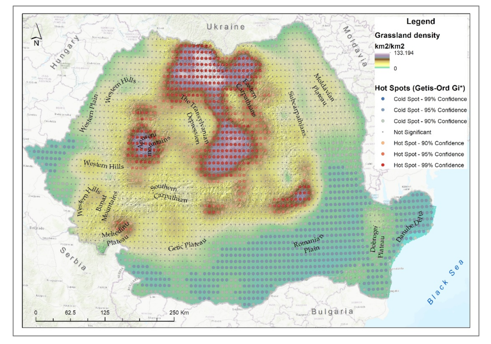
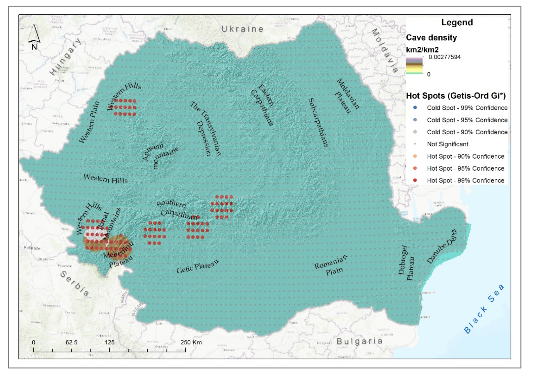
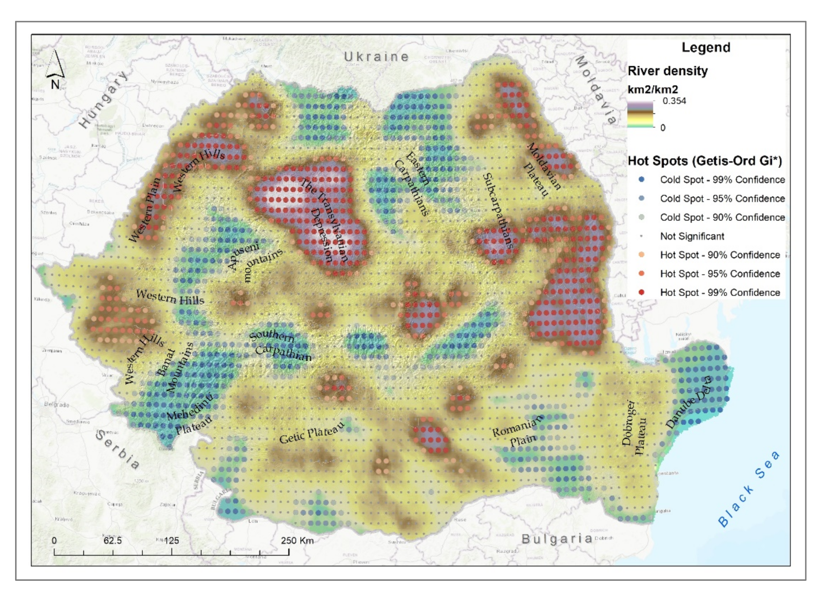
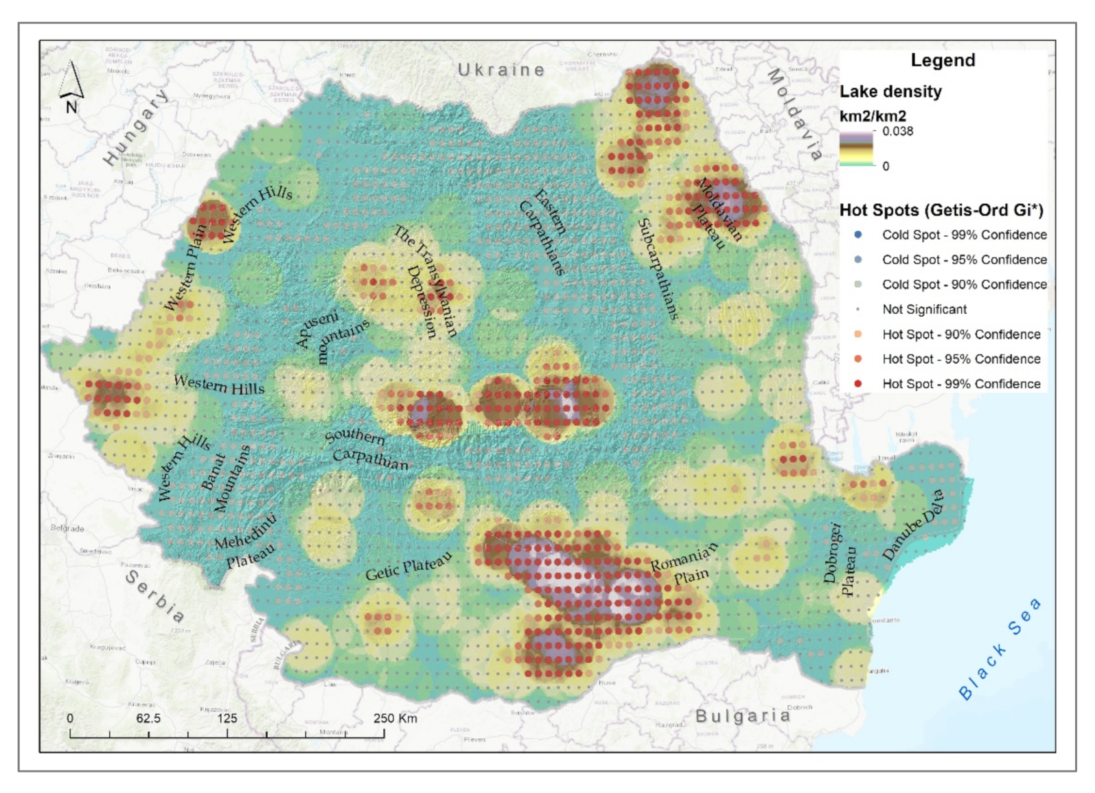
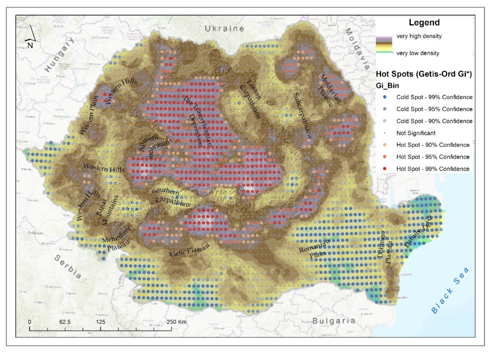
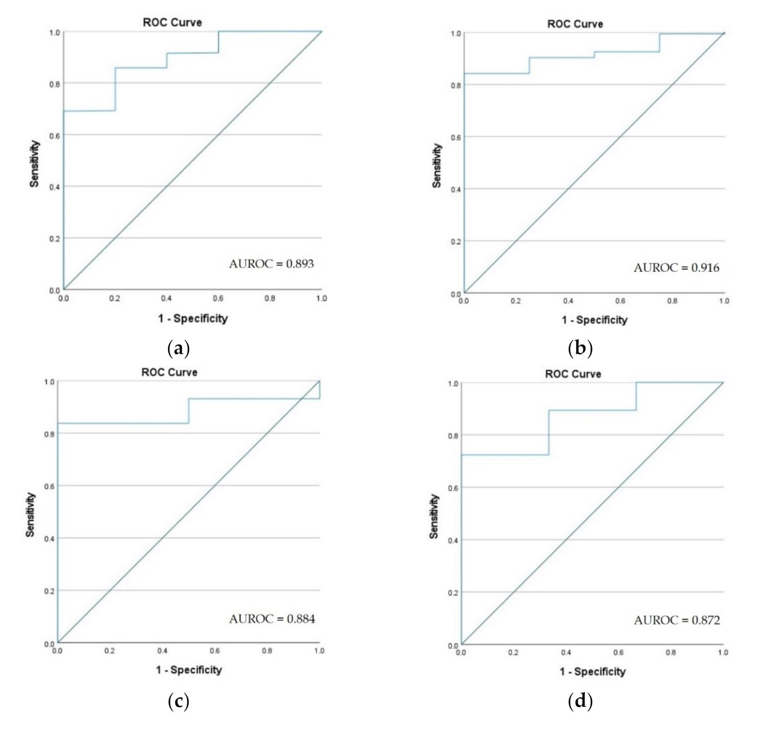
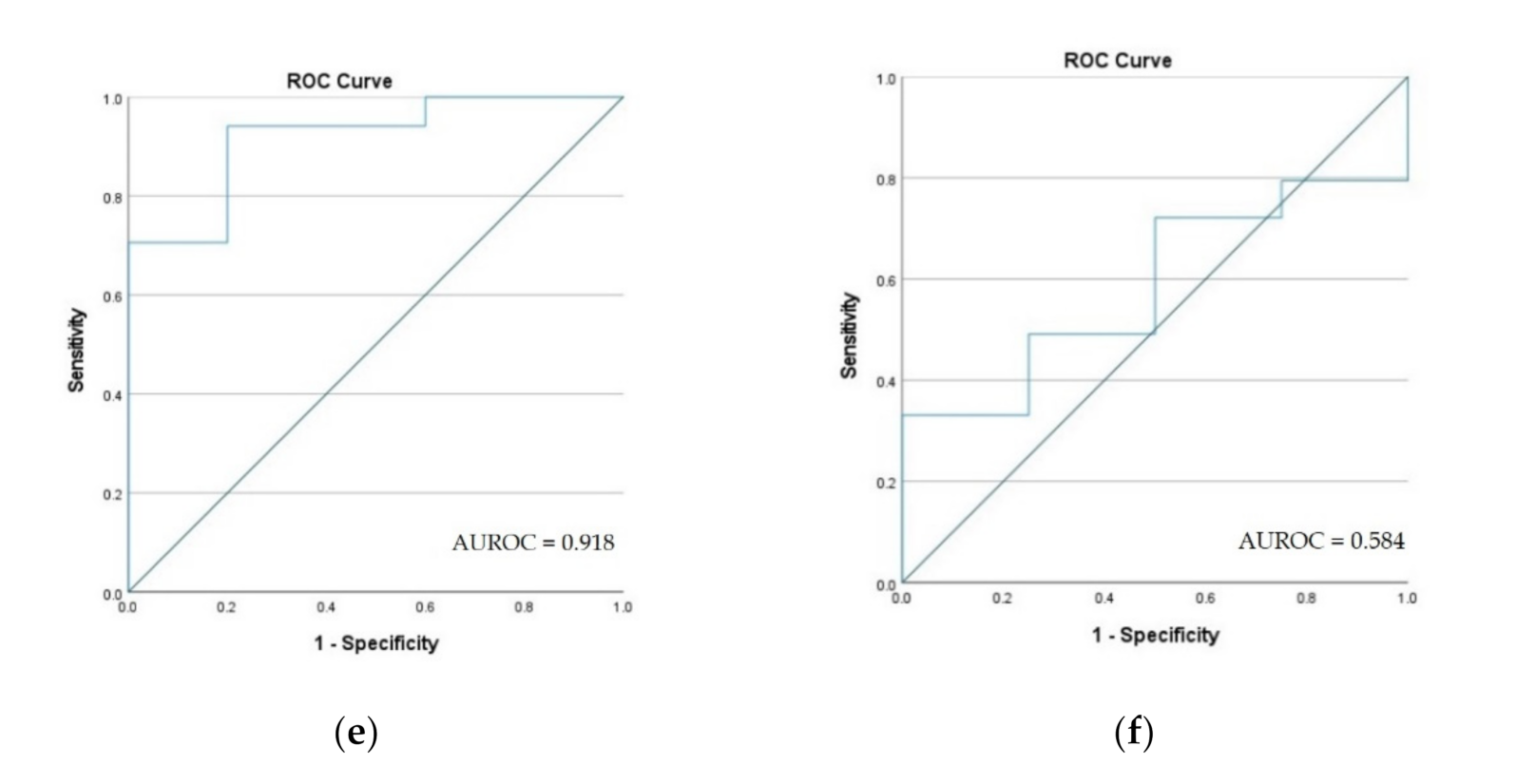
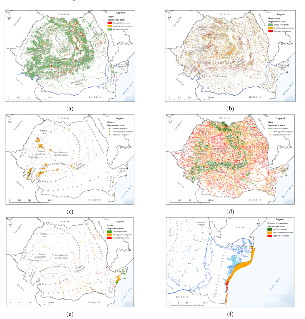
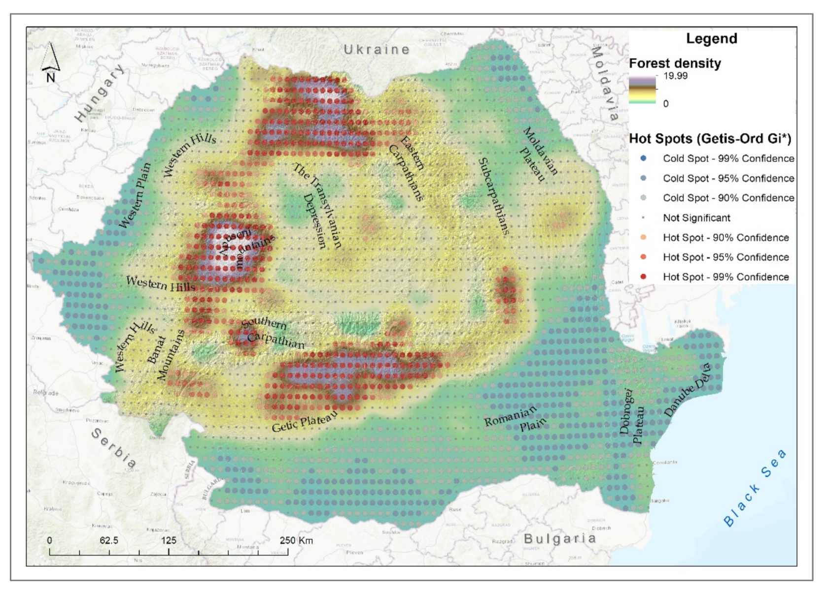
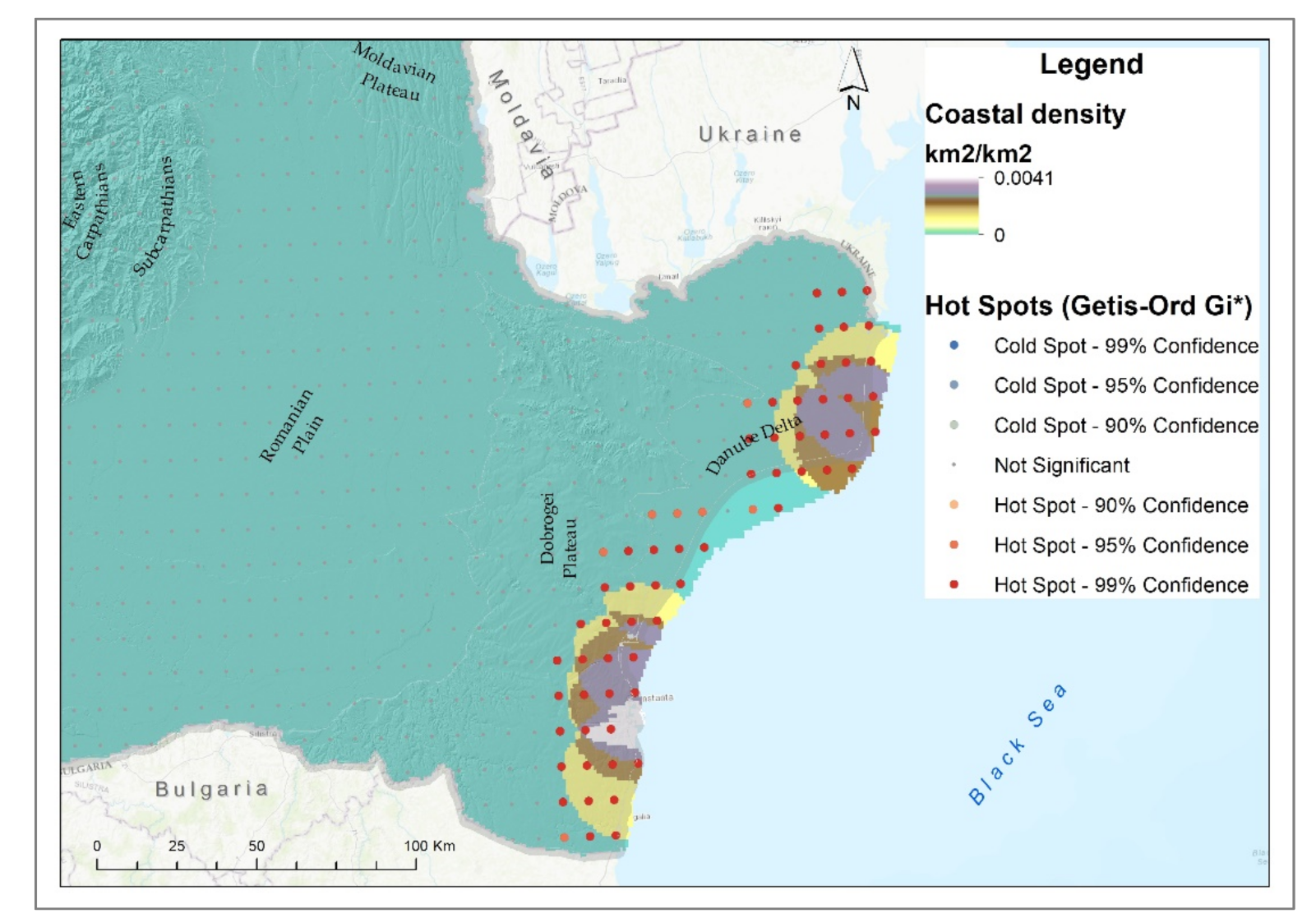
3. Results and Discussions

The integration of each Romanian ecosystem type assessment indicated that the coastal ecosystem is the most degraded ecosystem, with 86.55% degraded area (1362.32 km2). The grassland ecosystem’s evaluation resulted in classification of 38.59% area of grassland as being degraded (12,486.37 km2), while 27.64% of river ecosystems were degraded (23,800.22 km length),
A share of 92.92% of cave ecosystems were semi-degraded, followed by 67.67% for lakes and 52.94% for rivers.
Forest ecosystems occupy the largest area of all ecosystems, and a share of 88.54% of this ecosystem was natural, non-degraded. Thus, for the identification of degraded forests, the VCF MODIS sensor was used, which allowed the mapping of forests with a consistency between 30% and 80%, which showed a consistency reduction of over 10%. According to the analysis, only 8.52% of forest ecosystems were degraded (Table 2).
The largest area of forest ecosystems was located in the Carpathian Mountains, about 31% in the Eastern Carpathians, 16% in the Western Carpathians and 14% in the Southern Carpathians (Figure 3a). The largest degraded forest ecosystem areas were located in the Eastern Carpathian Mountains, area where deforestation hotspots have been identified in several similar studies [67,68]. The main cause is deforestation resulting in ecosystem loss and fragmentation. Approximately 1124 km2 were deforested in the Eastern Carpathians, from which 790 km2 were transformed into unproductive land, 652.5 km2 into pastures and 177 km2 into built-up areas. At the same time, significant forest areas were deforested in the Western Carpathians (approximately 320 km2) and the Southern Carpathians (256 km2). In the plateau and plain areas, the main cause of degradation was conversion to agricultural land.
The grasslands cover the second largest ecosystem area within Romanian territory (Figure 3b). The largest degraded area of the grassland ecosystem was in the Transylvanian Depression (approximately 2340 km2), followed by the Eastern Carpathians with approximately 2220 km2 and the Sub-Carpathians with 1433 km2. Similar studies on grassland degradation in the Sub-Carpathian area have drawn attention to the degradation rates of grassland in this area and the influence of this process in the manifestation of landslides [69]. These three landforms are concentrated on approximately 50% of the area of degraded grassland ecosystems in Romania. The causes are multiple, from the presence of invasive species such as shrubs to agro-pastoral activities such as excessive grazing.
Most of the cave ecosystems in Romania are located in the Western Carpathians (179 caves), followed by the Southern Carpathians (101 caves) and the Eastern Carpathians (21 caves), (Figure 3c). Most of the caves (50.4%) are located in the Continental biogeographic region, 47.8% in the temperate-continental climatic and 1.8% in the cold semi-arid climate (Dobrogea Plateau).
The assessment of the degree of cave degradation involved the assessment of the environmental and underground impact on the cave ecosystem’s environmental impact and underground impact (slope collapses that led to clogging of entrances or opening of new entrances, water catchments in the karst impluvium, constructions, communication routes in the perimeter of the cave, storage of household waste or other material, excessive and/or disorganized tourism), evaluation of the paleontological deposit—thanatocoenosis (fossil deposit affected by illegal excavations/vandalism, presence of vandalized bioglyphs), archeologic evaluation of the deposit (incisions/drawings with vandalized coal, stone/bone/metal tools destroyed or removed from the archaeological/sedimentological context), assessment of the biodiversity of the underground environment—invertebrate fauna, vertebrate fauna (depending on diversity specific to the fauna of vertebrates and invertebrates in caves).
The analysis showed that approximately 90% of the cave ecosystems were semi-degraded and only 2.66% were degraded.
Most rivers in Romania spring in the Carpathian Mountains, flowing into hilly areas (small rivers) and lowland areas (large rivers). Their condition is influenced by the physical–geographical and socioeconomic characteristics of the areas they pass through. The mountainous areas cover 46.2% of the length of the rivers in Romania, the hill and plateau area constitutes 35.8% and plain and Danube Delta areas 18%.
A preponderance of degraded and semi-degraded river ecosystems were observed in areas with low attitudes, in the plains (Figure 3d). There were approximately 4700 km of degraded rivers in the Romanian Plain and another 5000 km in a semi-degraded state, and 685 km were in a natural state.
In the Transylvanian Depression, approximately 4150 km were classified to a state of degradation, to which were added 5450 km in a state of semi-degradation, leaving only 390 km in a natural state.
Most lake ecosystems are located in the southeastern and eastern part of Romania, respectively, in the Danube Delta (43.1%), the Romanian Plain (22.17%), the Dobrogea Plateau (6.62%) and the Moldavian Plateau (5.39%), (Figure 3e). The largest degraded area of lake ecosystems was located in the Romanian Plain with an area of 177.06 km2, representing 35.52% of the lake ecosystems in this area, followed by the Moldavian Plateau with 45.9 km2 and the Dobrogea Plateau with 32.16 km2. Moreover, in the Dobrogea Plateau and in the Moldavian Plateau were the largest areas of semi-degraded lake ecosystems, 116.48 and 116.09 km2, respectively.
The largest degraded areas of coastal ecosystems were in the Periboina–Cap Singol area (71.05 km2), the Mangalia Plateau (20.34 km2) and the Chituc Grind (18.49 km2) (Figure 3f). The largest semi-degraded areas were in the areas Sulina–Periboina (963.83 km2), Periboina–Cap Singol (258.11 km2) and Eforie–Vama Veche (88.81 km2).
The highest density of degraded forest ecosystems was identified in the Northeastern Carpathians, the northern group of the Western Carpathians and in the Southern Carpathians and also in the Sub-Carpathians (Figure 4). Moreover, in these areas, the confidence level of the hotspot was over 99%. The extensive forest areas that were deforested in northern Romania, in the Maramureș Mountain area led to landscape degradation and decreased air quality and contributed to the aggravation of the negative effects of torrential floods due to the limited capacity to retain water in the canopy.
The highest density of degraded grassland ecosystems was identified in the Northeastern Carpathians, in the Transylvanian Depression, the north, central-eastern and southern parts, and the confidence level of the hotspot was over 99% (Figure 5). A high density was also observed in the Nordic group of the Western Carpathians.
The density of degraded cave ecosystems in Romania is very low; however, some hotspots can be observed in the south of the Western Carpathians and in the Southern Carpathians (Figure 6). Cold spots identified for mountain areas with a high density of caves in the case of the Apuseni Mountains were due to their low degradation, many of them presenting species from the Red List of Romanian cave fauna [70]. The hotspots identified for the degraded caves were concentrated in the northern Apuseni Mountains, the Banat Mountains, the southern Retezat and Parâng mountains, as well as in Fagaraș (Figure 6). In these areas, there are numerous caves with a high number of tourists, which increases in temperature by up to 2 degrees and increases the pathogenic microorganisms, as determined locally and in studies conducted for Muierilor Cave and Polovragi Cave (from Parâng Mountains) and Urșilor Cave and Meziad Cave (from Apuseni Mountain) [71].
The density of degraded river ecosystems was very high in the northern and central part of the Transylvanian Depression, in the northern half of the Western Plain but also in the south of the Moldavian Plateau (Figure 7). Statistically significant hotspots were also registered in the central northern part of the Romanian Plain, in the northeast of the Moldavian Plateau and in the south of the Eastern Carpathians.
The concentration of rivers in the high degradation class in the plain areas (Moldavian Plain located in northeastern Romania, Western Plain and center of the Romanian Plain) is caused by agricultural practices that lead to water pollution due to the use of climatic fertilizers and increase in salinization against the background of increasing average temperatures. In the case of the Transylvanian Depression, a high concentration of degraded areas was also identified. This area is known to be degraded due to the expansion of urban agglomerations but also because of the numerous rural settlements where the sewerage systems do not comply with the environmental regulations in force so that nitrogen pollution is high [72] so that the river degradation class is high.
The highest density of lake ecosystems was identified in the central part of the Romanian Plain, in the south of the Transylvanian Depression and in the north of the Moldavian Plateau (Figure 8). Statistically significant hotspots could also be observed in the Western Plain.
The analysis of the state of degradation of the coastal environment highlighted the areas of expansion of invasive species such as Ailanthus altissima, Amorpha fruticosa, Elaeagnus angustifolia and, from the category of marine species, Rapana venosa and Mnemiopsis leidyi [73].
The influence of wastewater discharges and the influence of tourist activities was visible for the terrestrial environment of the coastal area, noting in particular the coastal area south of the Dobrogea Plateau, as well as the south of the Danube Delta, territories where the density of tourist resorts is high, thus inducing a negative effect on the studied ecosystem (Figure 9).
Finally, by combining the densities of all the analyzed ecosystems, the map of the density of degraded ecosystems in Romania was obtained (Figure 10).
This highlights a statistically significant high density in the central part of the country due to the numerous natural meadows that are in a medium and high degradation stage due to the anthropogenic pressure on them, the high number of river segments that are in an advanced stage of degradation due to numerous sources of pollution mainly caused by the lack of septic tanks and the inefficient use of chemical fertilizers in agriculture and the south of the Carpathian Mountains, where, along with the declining forest, there are a high number of degraded meadows but also degraded river segments.
Statistically significant hotspots were also observed in the Moldavian Plateau and in the north of the Western Plain where there was a high number of degraded lakes and rivers as highlighted by the experts involved in the project on-site (Table 3).
Relative operating characteristics (ROC) analysis was used to determine the accuracy of determining the degradation stage for the six types of ecosystems analyzed. The method provides a curve given by a confusion matrix of binary classification according to four possible outcomes: true positive, true negative, false positive and false negative. The results are derived by comparing results of the model with the ground truth survey (GTS), which are established by through field campaigns carried out in spring, summer and autumn for all 6 types of ecosystems with the help of 35 environmental experts from the project, who aimed to identify the state of ecosystems with an emphasis on their degradation. Statistical analyses were conducted using the SPSS software program.
The outcomes are derived by comparing results of the model with the ground truth survey (GTS), approximately 100 points chosen randomly for each type of ecosystem so as to cover all the counties of Romania. The ROC curve is a method that compares true-positive rates against false-positive rates. For each random point, a buffer area of 300 m was analyzed to verify the presence or absence of degradation.
Following the analysis of ROC curves for the six types of degraded ecosystems, it can be seen that the models that have a high degree of representativeness for the analyzed problem were those that focused on identifying degraded ecosystems (characterized by a value of the area of under the ROC cure of 0.916) and the model for determining the degraded lakes (characterized by a value of the area under the ROC cure of 0.918) (Figure 11).
In the case of the models that targeted the ecosystems of forests, caves and rivers, lower values were calculated but located above the limit of 0.800, considered a threshold value in order to frame the results in the category of strong and moderate models [74]. However, these values are justified, taking into account the diversity of the causes of degradation as well as their uneven distribution at the national level [75]. The model with a low validation rate was the coastal ecosystems model for which improvements can be made in future studies, aimed at lowering the distinction between the distribution of disturbing factors on land and water and their dispersion with distance from shore [76]. However, we considered that, for the present study, we should keep all six models so that the final map of cumulative degradation of all ecosystems can be made at the national level and draw attention to hotspots that require detailed studies or case studies to analyze in time the current situation of degradation.

4. Conclusions

Identifying degraded ecosystems is a key element of the ecological reconstruction strategy. In this sense, their analysis contributes to a better understanding of the mechanisms that have led to changes in the structure and functioning of ecosystems, with a direct impact on ecosystem services. The conceptual approach based on the mapping and assessment of ecosystem services contributes significantly to the development of an integrated vision of ecological reconstruction.
Represented by the variety of ecosystems, species and genes, the biodiversity in Romania is the national natural capital, being an integral part of sustainable development, by providing goods and services such as food, carbon sequestration and redistribution of marine and terrestrial water, which underlie prosperity, economic development, social welfare and quality of life.
Human activities are assessed in terms of direct or indirect impact on the components of biological diversity in order to apply appropriate measures to minimize adverse effects, reconstruction, rehabilitation and remediation of affected ecosystems.
Considering the fact that for all 6 types of ecosystems a group of 35 environmental professionals performed field studies and identified the state of the ecosystems with an emphasis on their degradation, we consider that the database used reaches the degree of detail necessary to draw general conclusions in terms of the concentration of degraded areas in Romania. Following the hotspot analysis, it was identified that the largest degraded surfaces are the coastal ones (49.80%), followed by the grassland ecosystems (38.59%) and the cave ecosystems (2.66%), while the degraded rivers ecosystems are degraded by a proportion of 27.64%, degraded forest ecosystems by 8.52%, and degraded lakes ecosystems by 14.05%. Relative operating characteristics (ROC) analysis highlights that the models that have a high degree of representativeness are the grassland ecosystems (characterized by a value of the area of under the ROC curve of 0.916) and lake ecosystems (with ROC cure value of 0.918). Ecosystems characterized by a great diversity of the causes of degradation as well as their uneven distribution at the national level such as the ecosystems of forests, caves and rivers with a ROC value above the limit of 0.800.
The degradation of a particular ecosystem must be assessed by the characteristics of the ecosystem to be restored. The methodology for assessing the degree of degradation of ecosystems is based on a series of activities, criteria, methods and procedures for estimating the values of the parameters that indicate the state of these ecosystems. Therefore, it is important to discover the natural processes that take place in the system and to analyze the changes produced by the impact of anthropogenic activities. Conservation status assessment and monitoring consists of identifying direct or indirect risks and assessing the degree of habitat threat.
The study carried out on the changes that occurred in the natural environment on the Romanian territory shows how the deterioration and pollution of the areas is directly related both to the industrial activities in the area and to the inevitable climatic changes and other natural phenomena.
In conclusion, the highest density of degraded ecosystems in Romania is located in the central part, in the Transylvanian Depression and south of the Carpathian Mountains, in the Sub-Carpathians. The main factors that led to the degradation of ecosystems in Romania were anthropogenic but also natural.
This comprehensive study is an important step in the field of ecological reconstruction in Romania, as the starting point for future studies and supplementary rehabilitation actions.

Supplementary Materials

The following are available online at https://www.mdpi.com/article/10.3390/ijerph182111416/s1, Supplementary: Ecosystem services and type and sources of degradation used in this study.

Author Contributions

Conceptualization, S.A. and C.G.; methodology, S.A. and I.O.; software, I.O. and S.R. (Steliana Rodino); validation S.R. (Sanda Roșca); formal analysis, S.A. and C.G.; investigation, C.G., S.A. and I.O.; resources, C.G., S.A. and I.O.; data curation I.O. and S.R. (Steliana Rodino); writing—original draft preparation, S.A. and I.O,; writing—review and editing, S.R. (Sanda Roșca); visualization, I.O.; supervision, S.A. and C.G. All authors have read and agreed to the published version of the manuscript.

Funding

This research received no external funding.

Institutional Review Board Statement

Not applicable.

Informed Consent Statement

Not applicable.

Conflicts of Interest

The authors declare no conflict of interest.

References

  1. Chu, E.W.; Karr, J.R. Environmental impact: Concept, consequences, measurement. Ref. Modul. Life Sci. 2017. [Google Scholar] [CrossRef]
  2. Brumă, I.S. The evolution of organic agricultural land areas in the emerging countries of the European Union. Agric. Econ. Rural Dev. 2014, 11, 167–179. [Google Scholar]
  3. Malhi, Y.; Franklin, J.; Seddon, N.; Solan, M.; Turner, M.G.; Field, C.B.; Knowlton, N. Climate change and ecosystems: Threats, opportunities and solutions. Philos. Trans. R. Soc. B Biol. Sci. 2020, 375, 20190104. [Google Scholar] [CrossRef] [PubMed] [Green Version]
  4. Popescu, V.D.; Rozylowicz, L.; Niculae, I.M.; Cucu, A.L.; Hartel, T. Species, habitats, society: An evaluation of research supporting EU’s Natura 2000 network. PLoS ONE 2014, 9, e113648. [Google Scholar] [CrossRef] [PubMed] [Green Version]
  5. Rosca, S.-M.; Simonca, V.; Bilasco, S.; Vescan, I.; Fodorean, I.; Petrea, D.-P. The assessment of favourability and spatio-temporal dynamics of pinus mugo in the romanian carpathians using GIS technology and landsat images. Sustainability 2019, 11, 1–30. [Google Scholar] [CrossRef] [Green Version]
  6. Corpade, A.M.; Corpade, C.; Petrea, D.; Moldovan, C. Integrating environmental considerations into transportation planning through strategic environmental assessment. J. Settl. Spat. Plan. 2012, 3, 115–120. [Google Scholar]
  7. Plesnik, J.; Hosek, M.; Condé, S. A Concept of a Degraded Ecosystem in Theory and Practice—A Review; ETC/BD Report to the EEA; European Environment Agency: Paris, France, 2011; pp. 1–11. [Google Scholar]
  8. Ghazoul, J.; Burivalova, Z.; Garcia-Ulloa, J.; King, L.A. Conceptualizing forest degradation. Trends Ecol. Evol. 2015, 30, 622–632. [Google Scholar] [CrossRef] [PubMed]
  9. Maes, J.; Teller, A.; Erhard, M.; Grizzetti, B.; Barredo, J.I.; Paracchini, M.L.; Condé, S.; Somma, F.; Orgiazzi, A.; Jones, A.; et al. Mapping and Assessment of Ecosystems and their Services: An Analytical Framework for Ecosystem Condition; Publications Office of the European Union: Luxembourg, 2018; Available online: https://publications.europa.eu/en/publication-detail/-/publication/42d646b6-1c3a-11e8-ac73-01aa75ed71a1/language-en (accessed on 1 March 2021).
  10. Avram, S.; Croitoru, A.; Gheorghe, C.A.; Nicolae, M.; Badarau, S.A.; Barbos, I.M.; Radu, B.; Ciocanea, C.M.; Ciornei, L.; Corpade, A.M.; et al. Cartarea Ecosistemelor Naturale si Seminaturale Degradate; Romanian Academy Publishing House: Bucharest, Romania, 2018. [Google Scholar]
  11. Grădinaru, S.R.; Iojă, C.I.; Vânău, G.O.; Onose, D.A. Multi-dimensionality of land transformations: From definition to perspectives on land abandonment. Carpathian J. Earth Environ. Sci. 2020, 15, 167–177. [Google Scholar] [CrossRef]
  12. Senf, C.; Seidl, R. Mapping the forest disturbance regimes of Europe. Nat. Sustain. 2021, 4, 63–70. [Google Scholar] [CrossRef]
  13. Potapov, P.; Li, X.; Hernandez-Serna, A.; Tyukavina, A.; Hansen, M.C.; Kommareddy, A.; Pickens, A.; Turubanova, S.; Tang, H.; Silva, C.E.; et al. Mapping global forest canopy height through integration of GEDI and Landsat data. Remote Sens. Environ. 2021, 253, 112165. [Google Scholar] [CrossRef]
  14. Kumar, P.; Krishna, A.P.; Rasmussen, T.M.; Pal, M.K. Rapid Evaluation and validation method of above ground forest biomass estimation using optical remote sensing in tundi reserved forest area, India. ISPRS Int. J. Geo-Inf. 2021, 10, 29. [Google Scholar] [CrossRef]
  15. Williams, L.J.; Cavender-Bares, J.; Townsend, P.A.; Couture, J.J.; Wang, Z.; Stefanski, A.; Messier, C.; Reich, P.B. Remote spectral detection of biodiversity effects on forest biomass. Nat. Ecol. Evol. 2021, 5, 46–54. [Google Scholar] [CrossRef] [PubMed]
  16. Meng, B.; Liang, T.; Yi, S.; Yin, J.; Cui, X.; Ge, J.; Hou, M.; Lv, Y.; Sun, Y. Modeling alpine grassland above ground biomass based on remote sensing data and machine learning algorithm: A case study in east of the Tibetan Plateau, China. IEEE J. Sel. Top. Appl. Earth Obs. Remote. Sens. 2020, 13, 2986–2995. [Google Scholar] [CrossRef]
  17. Wu, J.; Liang, S. Assessing terrestrial ecosystem resilience using satellite leaf area index. Remote Sens. 2020, 12, 1–20. [Google Scholar] [CrossRef]
  18. Kang, W.; Wang, T.; Liu, S. The response of vegetation phenology and productivity to drought in semi-arid regions of northern China. Remote Sens. 2018, 10, 727. [Google Scholar] [CrossRef] [Green Version]
  19. Pastick, N.J.; Wylie, B.K.; Wu, Z. Spatiotemporal analysis of Landsat-8 and Sentinel-2 data to support monitoring of dryland ecosystems. Remote Sens. 2018, 10, 791. [Google Scholar] [CrossRef] [Green Version]
  20. Maurya, P.; Das, A.K.; Kumari, R. Managing the blue carbon ecosystem: A remote sensing and GIS approach. In Advances in Remote Sensing for Natural Resource Monitoring; Wiley Online Books: London, UK, 2021. [Google Scholar] [CrossRef]
  21. Woodgate, W.; Disney, M.; Armston, J.D.; Jones, S.D.; Suarez, L.; Hill, M.J.; Wilkes, P.; Soto-Berelov, M.; Haywood, A.; Mellor, A. An improved theoretical model of canopy gap probability for Leaf Area Index estimation in woody ecosystems. For. Ecol. Manag. 2015, 358, 303–320. [Google Scholar] [CrossRef]
  22. Li, Z.; Xu, D.; Guo, X. Remote sensing of ecosystem health: Opportunities, challenges, and future perspectives. Sensors 2014, 14, 21117–21139. [Google Scholar] [CrossRef] [Green Version]
  23. Weiskopf, S.R.; Rubenstein, M.A.; Crozier, L.G.; Gaichas, S.; Griffis, R.; Halofsky, J.E.; Hyde, K.J.W.; Morelli, T.L.; Morisette, J.T.; Muñoz, R.C.; et al. Climate change effects on biodiversity, ecosystems, ecosystem services, and natural resource management in the United States. Sci. Total Environ. 2020, 733, 137782. [Google Scholar] [CrossRef]
  24. Praticò, S.; Solano, F.; Di Fazio, S.; Modica, G. Machine learning classification of mediterranean forest habitats in google earth engine based on seasonal sentinel-2 time-series and input image composition optimisation. Remote Sens. 2021, 13, 586. [Google Scholar] [CrossRef]
  25. Yousefi, S.; Pourghasemi, H.R.; Avand, M.; Janizadeh, S.; Tavangar, S.; Santosh, M. Assessment of land degradation using machine-learning techniques: A case of declining rangelands. Land Degrad. Develop. 2021, 32, 1452–1466. [Google Scholar] [CrossRef]
  26. Papp, L.; van Leeuwen, B.; Szilassi, P.; Tobak, Z.; Szatmári, J.; Árvai, M.; Mészáros, J.; Pásztor, L. Monitoring invasive plant species using hyperspectral remote sensing data. Land 2021, 10, 29. [Google Scholar] [CrossRef]
  27. Roman, A.; Gafta, D. Proximity to successionally advanced vegetation patches can make all the difference to plant community assembly. Plant Ecol. Divers. 2013, 6, 269–278. [Google Scholar] [CrossRef]
  28. Palaiologou, P.; Essen, M.; Hogland, J.; Kalabokidis, K. Locating forest management units using remote sensing and geostatistical tools in north-central Washington, USA. Sensors 2020, 20, 2454. [Google Scholar] [CrossRef] [PubMed]
  29. Maes, J.; Teller, A.; Erhard, M.; Condé, S.; Vallecillo, S.; Barredo, J.I.; Paracchini, M.L.; Abdul Malak, D.; Trombetti, M.; Vigiak, O. et al. Mapping and Assessment of Ecosystems and their Services: An EU Ecosystem Assessment; JRC Science for Policy Report; Publications Office of the European Union: Ispra, Italy, 2020; p. 452. [CrossRef]
  30. European Commission. Directorate-General for the Environment. Mapping and Assessment of Ecosystems and their Services Mapping and Assessing the Condition of Europe’s Ecosystems: Progress and Challenges: 3rd Report—Final. 20 March 2016. Available online: https://doi.org/10.2779/351581 (accessed on 8 February 2021). [CrossRef]
  31. EC. Communication from the Commission to the European Parliament, the Council, the European Economic and Social Committee and the Committee of the Regions, EU Biodiversity Strategy for 2030; European Commission: Brussels, Belgium, 2020. [Google Scholar]
  32. Kottek, M.; Grieser, J.; Beck, C.; Rudolf, B.; Rubel, F. World map of the Köppen-Geiger climate classification updated. Meteorol. Z. 2006, 15, 259–263. [Google Scholar] [CrossRef]
  33. EEA. Biogeographical Regions [WWW Document]. 2016. Available online: https://www.eea.europa.eu/data-and-maps/data/biogeographical-regions-europe-3 (accessed on 10 February 2021).
  34. Winkler, M.; Lamprecht, A.; Steinbauer, K.; Hülber, K.; Theurillat, J.-P.; Breiner, F.; Choler, P.; Ertl, S.; Gutiérrez Girón, A.; Rossi, G.; et al. The rich sides of mountain summits—A pan-European view on aspect preferences of alpine plants. J. Biogeogr. 2016, 43, 2261–2273. [Google Scholar] [CrossRef]
  35. APIA. LPIS [WWW Document]. 2017. Available online: https://lpis.apia.org.ro (accessed on 14 January 2021).
  36. DiMiceli, C.; Carroll, M.; Sohlberg, R.; Kim, D.; Kelly, M.; Townshend, J. MOD44B MODIS/Terra Vegetation Continuous Fields Yearly L3 Global 250 m SIN Grid [WWW Document]. 2015. ASA EOSDIS Land Processes DAAC. Available online: https://doi.org/https://doi.org/10.5067/MODIS/MOD44B.006 (accessed on 9 February 2021). [CrossRef]
  37. Hansen, M.C.; Potapov, P.V.; Moore, R.; Hancher, M.; Turubanova, S.A.; Tyukavina, A.; Thau, D.; Stehman, S.V.; Goetz, S.J.; Loveland, T.R.; et al. High-resolution global maps of 21st-century forest cover change. Science 2013, 342, 850–853. [Google Scholar] [CrossRef] [Green Version]
  38. APIA. LPIS [WWW Document]. 2013. Available online: https://lpis.apia.org.ro (accessed on 11 February 2021).
  39. ANCPI. Geoportal [WWW Document]. 2017. Available online: http://geoportal.ancpi.ro/geoportal (accessed on 15 February 2021).
  40. EEA. EU-DEM [WWW Document]. Copernicus Land Monitoring Service. 2016. Available online: https://land.copernicus.eu/imagery-in-situ/eu-dem/eu-dem-v1-0-and-derived-products/eu-dem-v1.0/view (accessed on 3 January 2021).
  41. INS. The General Agricultural Census [WWW Document]. 2017. Available online: https://insse.ro/cms (accessed on 18 February 2021).
  42. JRC. European Settlement Map [WWW Document]. 2016. Available online: https://land.copernicus.eu/pan-european/GHSL/european-settlement-map/EU GHSL 2014/view (accessed on 22 February 2021).
  43. ESA. Copernicus Open Access Hub [WWW Document]. 2017. Available online: https://scihub.copernicus.eu/dhus/#/home (accessed on 28 March 2021).
  44. Natura 2000 Sites [WWW Document]. 2017. Available online: http://www.mmediu.ro/articol/date-gis/434 (accessed on 20 December 2020).
  45. EEA. Corine Land Cover (CLC) 2012 [WWW Document]. 2016. Available online: http://land.copernicus.eu/pan-european/corine-land-cover/clc-2012/view (accessed on 16 December 2020).
  46. EEA. European Catchments and Rivers Network System (Ecrins) [WWW Document]. 2012. Available online: https://www.eea.europa.eu/data-and-maps/data/european-catchments-and-rivers-network (accessed on 14 November 2020).
  47. OSM. Open Street Map [WWW Document]. 2017. Available online: https://download.geofabrik.de (accessed on 4 April 2021).
  48. EEA. EU-Hydro—River Network Database [WWW Document]. 2017. Available online: https://land.copernicus.eu/imagery-in-situ/eu-hydro/eu-hydro-river-network-database (accessed on 11 December 2020).
  49. EEA. Riparian Zones 2012—Land Use Land Cover [WWW Document]. 2012. Available online: http://land.copernicus.eu/local/riparian-zones/land-cover-land-use-lclu-image/view (accessed on 9 November 2020).
  50. EEA. Waterbase—UWWTD: Urban Waste Water Treatment Directive [WWW Document]. 2015. Available online: https://www.eea.europa.eu/data-and-maps/data/waterbase-uwwtd-urban-waste-water-treatment-directive (accessed on 6 February 2021).
  51. INCPA. Romania Soils Map [WWW Document]. 2017. Available online: https://www.icpa.ro (accessed on 2 April 2021).
  52. INS. Number of Inhabitants [WWW Document]. 2017. Available online: https://insse.ro/cms (accessed on 7 November 2020).
  53. NASA USGS. EarthExplorer [WWW Document]. 2017. Available online: https://earthexplorer.usgs.gov (accessed on 17 November 2020).
  54. Niculae, M.I.; Avram, S.; Vanau, G.O.; Patroescu, M. Effectiveness of Natura 2000 network in Romanian Alpine Biogeographical Region: An assessment based on forest landscape connectivity. Ann. For. Res. 2014, 60, 19–32. [Google Scholar] [CrossRef] [Green Version]
  55. Roman, A.; Ursu, T.-M.; Onțel, I.; Marușca, T.; Grigore Pop, O.; Milanovici, S.; Sin-Schneider, A.; Adriana Gheorghe, C.; Avram, S.; Fărcaș, S.; et al. Deviation from grazing optimum in the grassland habitats of Romania within and outside the natura 2000 network. In Habitats of the World—Biodiversity and Threats; IntechOpen: London, UK, 2019. [Google Scholar] [CrossRef] [Green Version]
  56. Donato, C.R.; Ribeiro AD, S.; Souto, L.D.S. A conservation status index, as an auxiliary tool for the management of cave environments. Int. J. Speleol. 2014, 43, 315–322. [Google Scholar] [CrossRef] [Green Version]
  57. Avram, S.; Ciuinel, A.M.; Iu, C.; Manolache, A.M.; Negreanu, S.Ș.; Manta, N. Applying a new methodology for cave degradation assessment in Romania—Case study on Rodna Mountains National Park. Extrem. Life Biospeol. Astrobiol. 2017, 9, 22–31. [Google Scholar]
  58. Ciocănea, C.M.; Corpade, P.C.; Onose, D.A.; Vânău, G.O.; Maloş, C.; Petrovici, M.; Gheorghe, C.; Dedu, S.; Manta, N.; Szép, R.E. The assessment of lotic ecosystems de Fgradation using multi-Criteria analysis and gis techniques. Carpathian J. Earth Environ. Sci. 2019, 14, 255–268. [Google Scholar] [CrossRef]
  59. Romanelli, A.; Esquius, K.S.; Massone, H.E.; Escalante, A.H. GIS-based pollution hazard mapping and assessment framework of shallow lakes: Southeastern Pampean lakes (Argentina) as a case study. Environ. Monit. Assess. 2013, 185, 6943–6961. [Google Scholar] [CrossRef]
  60. Mirzaei, M.; Solgi, E.; Salman-Mahiny, A. Evaluation of surface water quality. Arch. Hyg. Sci. 2016, 5, 265–277. [Google Scholar]
  61. Niculae, M.I.; Avram, S.; Corpade, A.M.; Dedu, S.; Gheorghe, C.A.; Pascu, I.S.; Ontel, I.; Rodino, S. Evaluation of the quality of lentic ecosystems in Romania by a GIS based WRASTIC model. Scient. Rep. 2021, 11, 1–10. [Google Scholar] [CrossRef]
  62. Avram, S.; Cipu, C.; Corpade, A.-M.; Gheorghe, C.A.; Manta, N.; Niculae, M.-I.; Pascu, I.S.; Szép, R.E.; Rodino, S. GIS-Based multi-criteria analysis method for assessment of lake ecosystems degradation—Case study in Romania. Int. J. Environ. Res. Public Health 2021, 18, 5915. [Google Scholar] [CrossRef] [PubMed]
  63. Getis, A.; Ord, J.K. The analysis of spatial association by use of distance statistics. Geogr. Anal. 1992, 24, 189–206. [Google Scholar] [CrossRef]
  64. Ord, J.K.; Getis, A. Local spatial autocorrelation statistics: Distributional issues and an application. Geogr. Anal. 1995, 27, 286–306. [Google Scholar] [CrossRef]
  65. Sánchez-Martín, J.M.; Rengifo-Gallego, J.I.; Blas-Morato, R. Hot spot analysis versus cluster and outlier analysis: An enquiry into the grouping of rural accommodation in Extremadura (Spain). ISPRS Int. J. Geo-Inf. 2019, 8, 176. [Google Scholar] [CrossRef] [Green Version]
  66. ESRI. How Hot Spot Analysis (Getis-Ord Gi*) Works [WWW Document]. 2020. Available online: https://desktop.arcgis.com/en/arcmap/10.3/tools/spatial-statistics-toolbox/h-how-hot-spot-analysis-getis-ord-gi-spatial-stati.htm (accessed on 21 April 2021).
  67. Griffiths, P.; Kuemmerle, T.; Baumann, M.; Radeloff, V.C.; Abrudan, I.V.; Lieskovsky, J.; Hostert, P. Forest disturbances, forest recovery, and changes in forest types across the Carpathian ecoregion from 1985 to 2010 based on Landsat image composites. Remote Sens. Environ. 2014, 151, 72–88. [Google Scholar] [CrossRef]
  68. Drăgan, M.; Mureşan, G.-A.; Benedek, J. Mountain wood-pastures and forest cover loss in Romania. J. Land Use Sci. 2020, 14, 397–409. [Google Scholar] [CrossRef]
  69. Malek, Z.; Zumpano, V.; Haydar, H. Forest management and future changes to ecosystem services in the Romanian Carpathians. Environ. Dev. Sustain. 2018, 20, 1275–1291. [Google Scholar] [CrossRef] [Green Version]
  70. Moldovan, O.T.; Iepure, S.; Brad, T.; Kenesz, M.; Mirea, I.C.; Năstase-Bucur, R. Database of Romanian cave invertebrates with a Red List of cave species and a list of hotspot/coldspot caves. Biodivers. Data J. 2020, 8, e53571. [Google Scholar] [CrossRef] [PubMed]
  71. Constantin, S.; Mirea, I.C.; Petculescu, A.; Arghir, R.A.; Măntoiu, D.S.; Kenesz, M.; Robu, M.; Moldovan, O.T. Monitoring human impact in show caves. A study of four Romanian caves. Sustainability 2021, 13, 1619. [Google Scholar] [CrossRef]
  72. World Bank. Romania Water Diagnostic Report: Moving toward EU Compliance, Inclusion, and Water Security; World Bank: Washington, DC, USA, 2018. [Google Scholar]
  73. Sitar, C.; Barbu-Tudoran, L.; Moldovan, O.T. Morphological and micromorphological description of the larvae of two endemic species of duvalius (Coleoptera, Carabidae, Trechini). Biology 2021, 10, 627. [Google Scholar] [CrossRef] [PubMed]
  74. Moresi, F.V.; Maesano, M.; Collalti, A.; Sidle, R.C.; Matteucci, G.; Scarascia Mugnozza, G. Mapping landslide prediction through a GIS-based model: A case study in a catchment in southern Italy. Geosciences 2020, 10, 309. [Google Scholar] [CrossRef]
  75. Hysa, A.; Spalevic, V.; Dudic, B.; Roșca, S.; Kuriqi, A.; Bilașco, Ș.; Sestras, P. Utilizing the available open-source remotely sensed data in assessing the wildfire ignition and spread capacities of vegetated surfaces in Romania. Remote Sens. 2021, 13, 2737. [Google Scholar] [CrossRef]
  76. Shidong, Z. Concept of Ecosystem Services and Ecosystem Management; Springer: Berlin/Heidelberg, Germany, 2013. [Google Scholar] [CrossRef]
Figure 1. Location of Romania and major landforms.
Ijerph 18 11416 g001
Figure 2. Methodological flow in order to assess the state of ecosystem degradation.
Ijerph 18 11416 g002
Figure 3. Distribution of ecosystems in Romania: (a) forest ecosystems; (b) grassland ecosystems; (c) cave ecosystems; (d) river ecosystems; (e) lake ecosystems; (f) coastal ecosystems.
Ijerph 18 11416 g003
Figure 4. Forest degraded ecosystem density and hotspot analysis.
Ijerph 18 11416 g004
Figure 5. Grassland degraded ecosystem density and hotspot analysis.
Ijerph 18 11416 g005
Figure 6. Cave degraded ecosystem density and hotspot analysis.
Ijerph 18 11416 g006
Figure 7. River degraded ecosystem density and hotspot analysis.
Ijerph 18 11416 g007
Figure 8. Lake degraded ecosystem density and hotspot analysis.
Ijerph 18 11416 g008
Figure 9. Coastal degraded ecosystem density and hotspot analysis.
Ijerph 18 11416 g009
Figure 10. Density of degraded ecosystems and hotspot analysis.
Ijerph 18 11416 g010
Figure 11. Relative operating characteristics (ROC) curve and AUROC value for degraded ecosystems. (a) Forest ecosystems; (b) grassland ecosystems; (c) cave ecosystems; (d) river ecosystems; (e) lake ecosystems; (f) coastal ecosystems.
Ijerph 18 11416 g011aIjerph 18 11416 g011b
Table 1. Used geo-database.
Major Ecosystem CategoryEcosystem Type for Mapping and AssessmentName of DatasetsResolution/Minimum Mapping UnitTime ReferenceSource
TerrestrialForestLand-parcel identification system (LPIS)NA2013Land-parcel identification system from Romania [35]
Vegetation Continuous Fields (MOD44B)250 m2000–2013LAADS DAAC [36]
Hansen Global Forest Change30 m2000–2013Global Forest Change [37]
GrasslandLand-parcel identification system (LPIS)NA2017Land-parcel identification system from Romania [38]
Limits of territorial administrative units (TAUs)NA2016National Agency for Cadastre and Land Registration of Romania [39]
Digital surface model (EU-DEM)25 m2011Copernicus Land Monitoring Service [40]
Livestock numbers and types from TAUsNA2010National Statistics Institute of Romania [41]
European Settlement Map10 m2010–2013Copernicus Land Monitoring Service [42]
Sentinel 2 images10 m2015–2017Copernicus Open-Access Hub [43]
CaveNatura 2000 (N2K)NA2017Ministry of Environment, Waters and Forests [44]
Orthophotos0.5 m2016National Agency for Cadastre and Land Registration of Romania [39]
CORINE Land Cover (CLC 2012)100 m2011–2012Copernicus Land Monitoring Service [45]
European Settlement Map10 m2010–2013Copernicus Land Monitoring Service [42]
European catchments and Rivers network system (ECRINS—dams on rivers)1:250,0002012European Environment Agency [46]
Roads and railwaysNA2016Open Street Map [47]
Fresh waterRiversEU-Hydro—River Network1 ha2006–2012Copernicus Land Monitoring Service [48]
European catchments and Rivers network system (ECRINS—dams on rivers)1:250,0002012European Environment Agency [46]
Digital surface model (EU-DEM)25 m2011Copernicus Land Monitoring Service [49]
CORINE Land Cover (CLC 2012)100 m2011–2012Copernicus Land Monitoring Service [45]
European Settlement Map10 m2010–2013Copernicus Land Monitoring Service [42]
Riparian Zones 2012—Land Use Land Cover0.5 ha2011–2013Copernicus Land Monitoring Service [49]
Urban Wastewater Treatment (Water-based UWWTD)NA2015European Environment Agency [50]
Natura 2000 (N2K)NA2017Ministry of Environment, Waters and Forests [44]
Roads and railwaysNA2016Open Street Map [47]
Romania soils mapNA2017National Institute of Research and Development for Pedology, Agro-chemistry and Environmental Protection [51]
Number of inhabitants from TAUsNA2017National Statistics Institute of Romania [52]
Limits of territorial administrative units (TAUs)NA2016National Agency for Cadastre and Land Registration of Romania [39]
LakesPermanent water bodies20 m2012Copernicus Land Monitoring Service
CORINE Land Cover (CLC 2012)100 m2011–2012Copernicus Land Monitoring Service [45]
Digital surface model (EU-DEM)25 m2011Copernicus Land Monitoring Service [40]
Roads and railwaysNA2016Open Street Map [47]
Exploitation areas of natural resourcesNA2017National Agency for Mineral Resources
Natura 2000 (N2K)NA2017Ministry of Environment, Waters and Forests [44]
Romania soils mapNA2017National Institute of Research and Development for Pedology, Agro-chemistry and Environmental Protection [51]
Urban Wastewater Treatment (Waterbased UWWTD)NA2015European Environment Agency [50]
Limits of territorial administrative units (TAUs)NA2016National Agency for Cadastre and Land Registration of Romania [39]
Landsat 830 m2016[53]
MarineCoastalCORINE Land Cover (CLC 2012)100 m2011–2012Copernicus Land Monitoring Service [45]
Digital surface model (EU-DEM)25 m2011Copernicus Land Monitoring Service [40]
Roads and railwaysNA2016Open Street Map [47]
Urban Wastewater Treatment (Waterbased UWWTD)NA2015European Environment Agency [50]
European Settlement Map10 m2010–2013Copernicus Land Monitoring Service [42]
Landsat 830 m2016[53]
Orthophotos0.5 m2016National Agency for Cadastre and Land Registration of Romania [39]
Table 2. Summary of ecosystem assessment results.
EcosystemNatural%Semi-Degraded%Degraded%Total
Forest (km2)63,651.3488.542115.272.946124.238.5271,890.84
Grassland (km2)7080.0521.8812,790.7239.5312,486.3738.5932,357.14
Cave (no.)154.4231592.9292.66339
Lake (km2)410.9518.281521.4167.67315.9114.052248.28
River (km)16,320.5219.4144,508.8252.942238.8227.6484,068.17
Coastal (km2)42.52.71362.3286.55169.1749.81574
Table 3. Classification of relief units in Romania by degradation classes.
Degradation.Low
(1–11)
Medium
(11–15)
High
(15–22)
Relief Unitskmp%kmp%kmp%
Eastern Carpathians2778.98.123,597.668.77949.823.2
Southern Carpathians2759.619.57120.750.34265.830.2
Banat Mountains1747.825.14448.463.8780.311.2
Sub-Carpathians215.51.36884.741.59473.057.2
Apuseni Mountains275.62.65976.256.14399.741.3
Transylvanian Depression0.00.02079.08.223,183.691.8
The Western Hills951.67.48034.862.73825.729.9
Mehedinti Plateau18.12.3519.565.1259.732.6
The Getic Plateau1879.413.67247.752.64654.933.8
The Plateau of Moldova1215.95.312,506.054.89091.939.9
Western Camp4059.425.310,012.962.32001.912.5
The Romanian Plain24,664.950.622,218.345.51903.23.9
Dobrogea Plateau6587.665.13424.233.8105.51.0
The Danube Delta4403.199.043.11.00.00.0
Low, medium and high classes were obtained using a natural-break classification of the density of degraded raster ecosystems presented in Figure 10.
Publisher’s Note: MDPI stays neutral with regard to jurisdictional claims in published maps and institutional affiliations.

