
Evaluating Spatiotemporal Distribution of Residential Sprawl and Influencing Factors Based on Multi-Dimensional Measurement and GeoDetector Modelling


Abstract
:1. Introduction
2. Materials and Methods
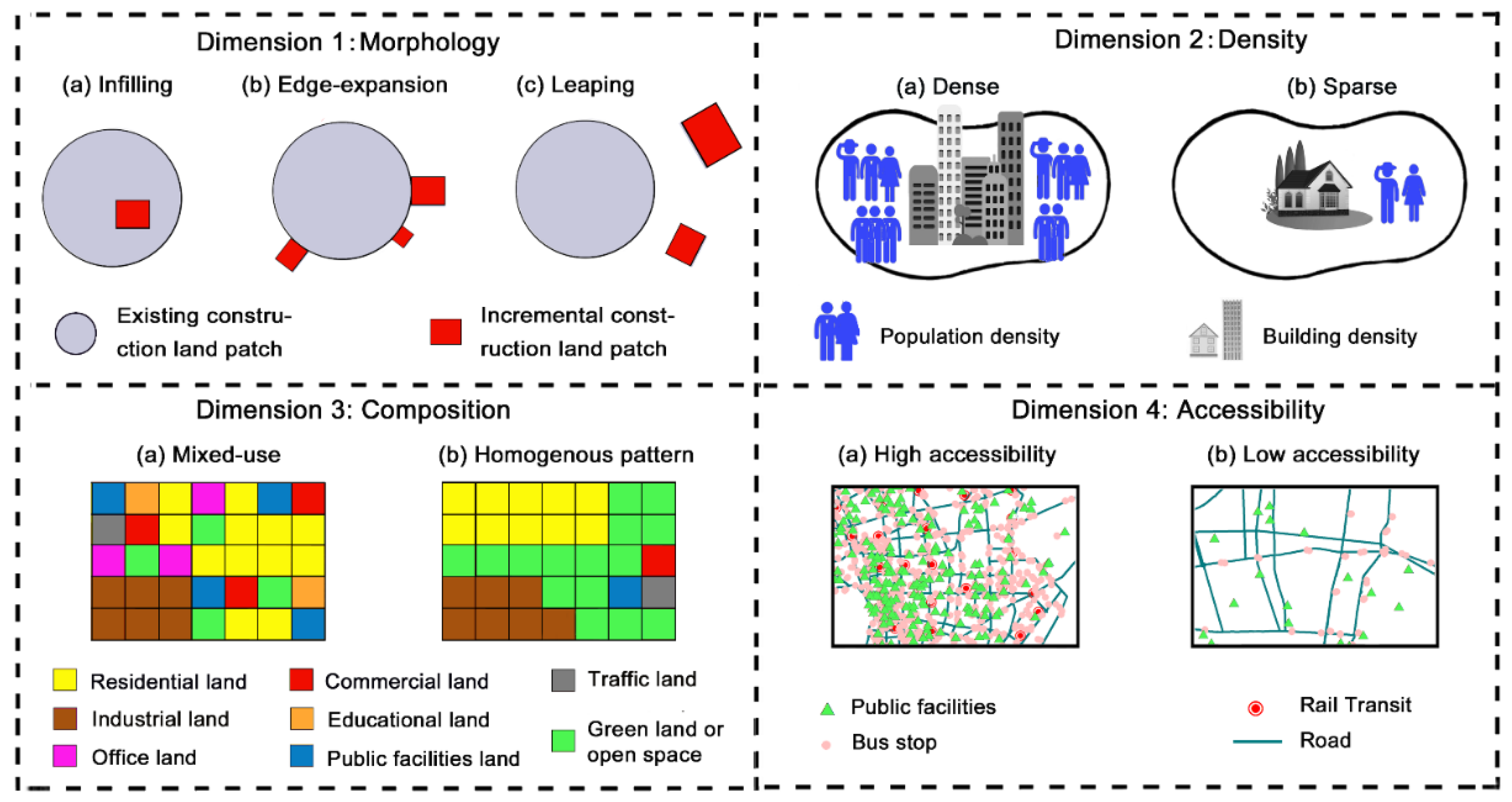
2.1. Multi-Dimensional Measurement
2.1.1. Sprawl Index
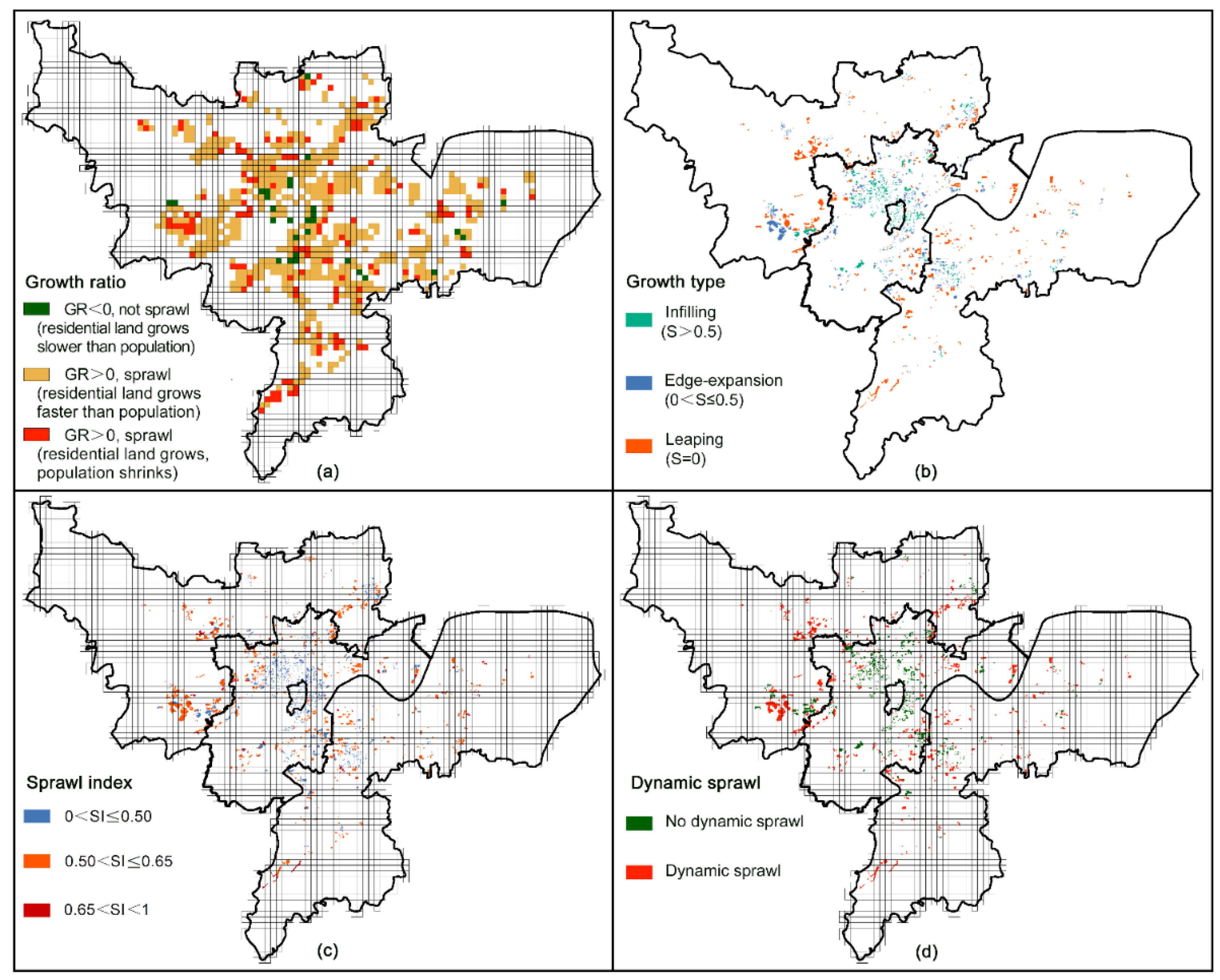
2.1.2. Dynamic Assessment
2.2. GeoDetector Modelling
2.2.1. Factor Detector
2.2.2. Interaction Detector
2.2.3. Variables
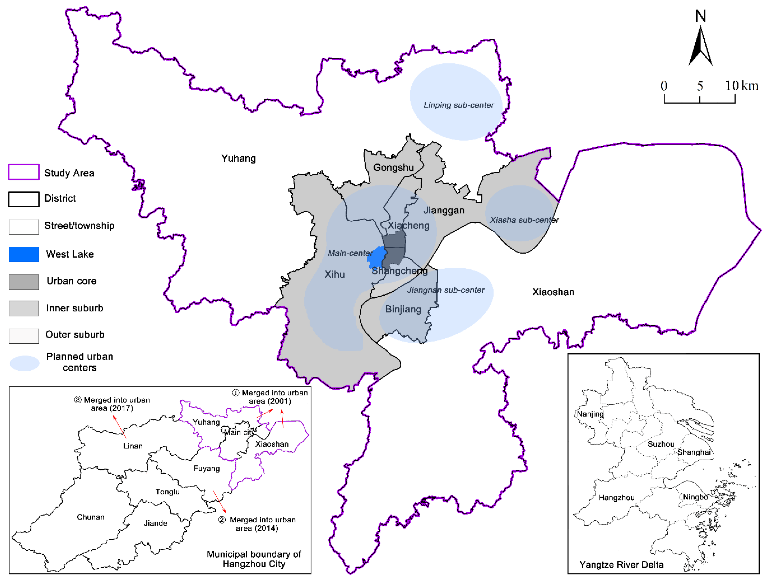
2.3. Study Area
3. Results
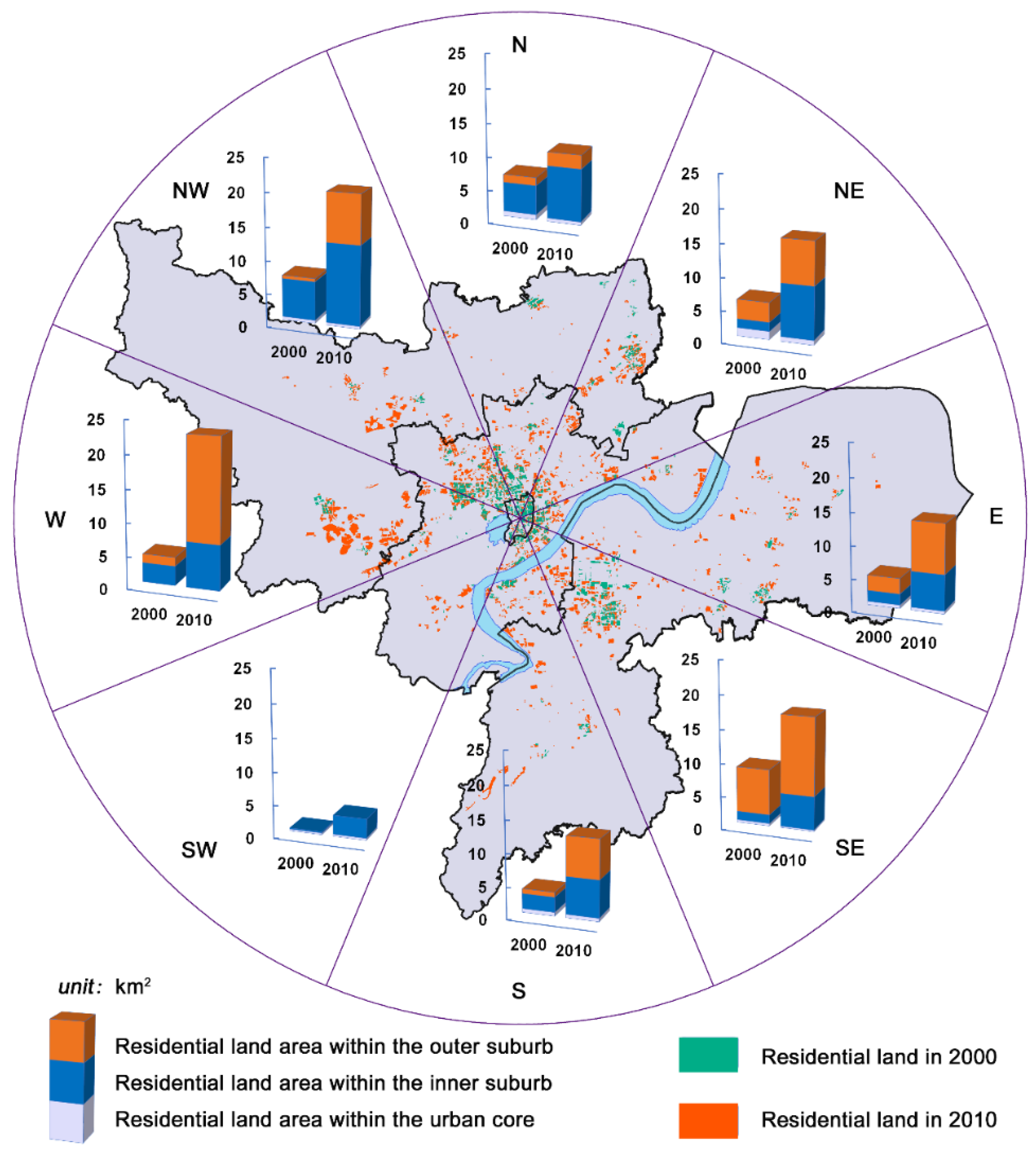
3.1. Multi-Dimensional Sprawl Index on Residential Land Cells
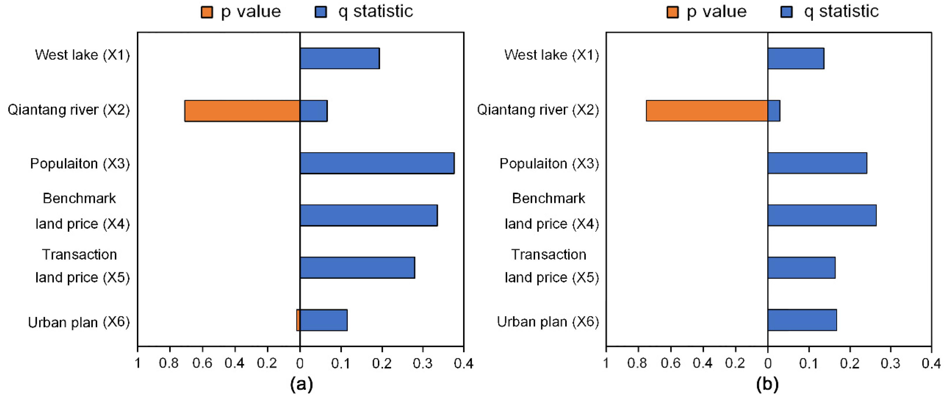
3.2. Influencing Factors for the Spatial Variation of SI
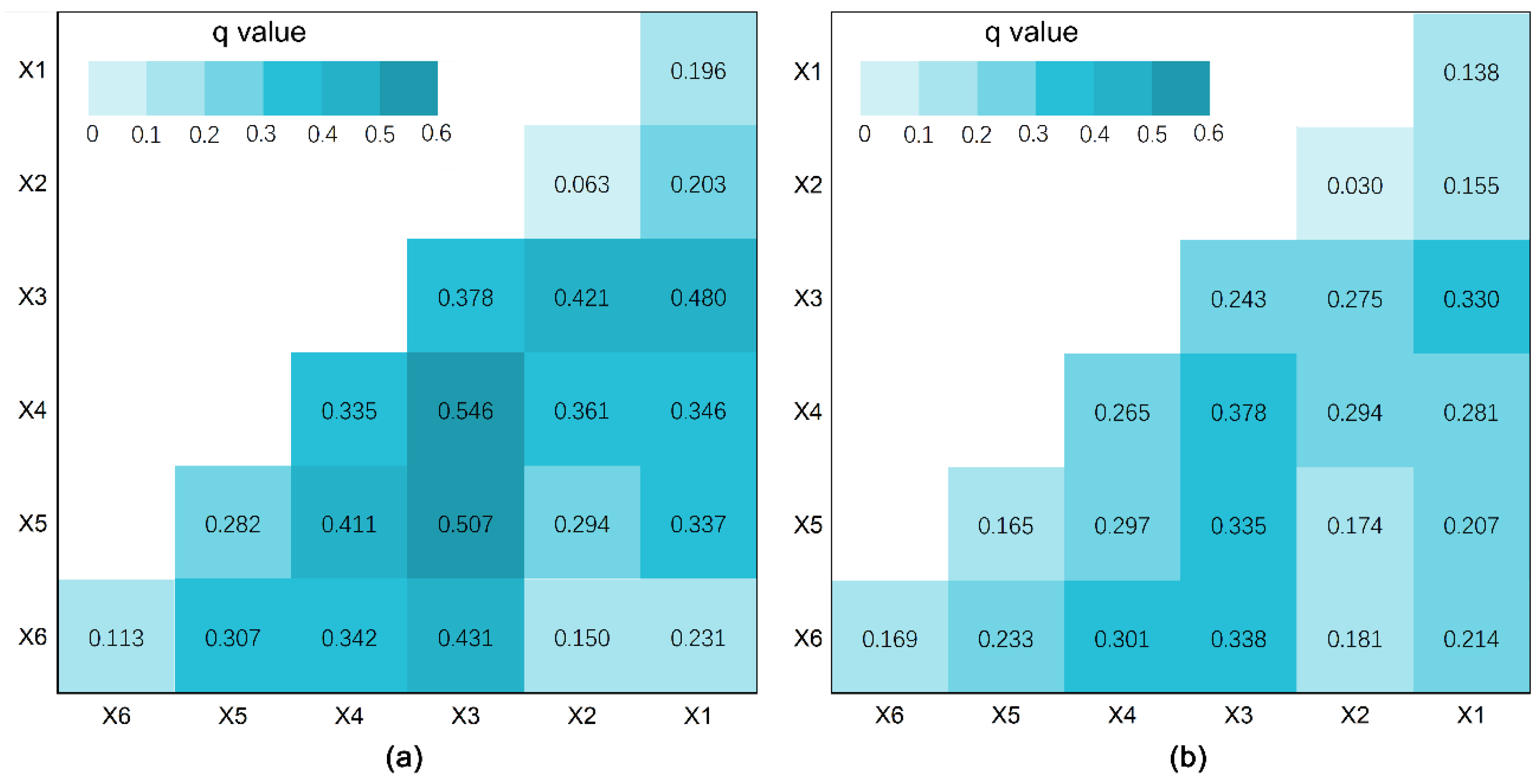
3.3. Interaction between Factors for Residential Sprawl
4. Discussion
4.1. Environment-Health Costs of Residential Sprawl
4.2. Effects of Urbanization, Land Market and Incremental Planning
4.3. Implications for Containing Residential Sprawl
5. Conclusions
Author Contributions
Funding
Institutional Review Board Statement
Informed Consent Statement
Data Availability Statement
Conflicts of Interest
References
- Friedmann, J. China’s Urbanization. Int. J. Urban Reg. Res. 2003, 27, 745–758. [Google Scholar] [CrossRef]
- Chen, M.; Liu, W.; Tao, X. Evolution and assessment on China’s urbanization 1960–2010: Under-urbanization or over-urbanization? Habitat Int. 2013, 38, 25–33. [Google Scholar] [CrossRef]
- Ewing, R.H. Characteristics, Causes, and Effects of Sprawl: A Literature Review. In Urban Ecology: An International Perspective on the Interaction Between Humans and Nature; Marzluff, J.M., Shulenberger, E., Endlicher, W., Alberti, M., Bradley, G., Ryan, C., Simon, U., ZumBrunnen, C., Eds.; Springer: Boston, MA, USA, 2008; pp. 519–535. [Google Scholar]
- Zhao, P. Sustainable urban expansion and transportation in a growing megacity: Consequences of urban sprawl for mobility on the urban fringe of Beijing. Habitat Int. 2010, 34, 236–243. [Google Scholar] [CrossRef]
- Yu, X.J.; Ng, C.N. Spatial and temporal dynamics of urban sprawl along two urban–rural transects: A case study of Guangzhou, China. Landsc. Urban Plan. 2007, 79, 96–109. [Google Scholar] [CrossRef]
- Tian, L.; Li, Y.; Yan, Y.; Wang, B. Measuring urban sprawl and exploring the role planning plays: A shanghai case study. Land Use Policy 2017, 67, 426–435. [Google Scholar] [CrossRef]
- Feng, L.; Du, P.J.; Li, H.; Zhu, L.J. Measurement of Urban Fringe Sprawl in Nanjing between 1984 and 2010 Using Multidimensional Indicators. Geogr. Res. 2015, 53, 184–198. [Google Scholar] [CrossRef]
- Liu, Y.; Fan, P.; Yue, W.; Song, Y. Impacts of land finance on urban sprawl in China: The case of Chongqing. Land Use Policy 2018, 72, 420–432. [Google Scholar] [CrossRef]
- Yue, W.; Liu, Y.; Fan, P. Measuring Urban Sprawl and Its Drivers in Large Chinese Cities: The Case of Hangzhou. Land Use Policy 2013, 31, 358–370. [Google Scholar] [CrossRef]
- Zhang, L.; Yue, W.; Liu, Y.; Fan, P.; Wei, Y.D. Suburban industrial land development in transitional China: Spatial restructuring and determinants. Cities 2018, 78, 96–107. [Google Scholar] [CrossRef]
- Wei, Y.H.D. Restructuring for growth in urban China: Transitional institutions, urban development, and spatial transformation. Habitat Int. 2012, 36, 396–405. [Google Scholar] [CrossRef]
- Shen, J.; Wu, F. Moving to the suburbs: Demand-side driving forces of suburban growth in China. Environ. Plan. A 2013, 45, 1823–1844. [Google Scholar] [CrossRef]
- Ewing, R.; Pendall, R.; Chen, D. Measuring Sprawl and Its Impact; Smart Growth America: Washington, DC, USA, 2002. [Google Scholar]
- Lopez, R.; Hynes, H.P. Sprawl in the 1990s Measurement, Distribution, and Trends. Urban Aff. Rev. 2003, 38, 325–355. [Google Scholar] [CrossRef] [PubMed]
- Hennig, E.I.; Soukup, T.; Orlitova, E.; Schwick, C.; Kienast, F.; Jaeger, J. Urban Sprawl in Europe. Joint EEA-FOEN Report. No 11/2016; European Environment Agency: København, Denmark, 2016.
- Navamuel, E.L.; Rubiera Morollón, F.; Moreno Cuartas, B. Energy consumption and urban sprawl: Evidence for the Spanish case. J. Clean. Prod. 2018, 172, 3479–3486. [Google Scholar] [CrossRef]
- Chan, C.K.; Yao, X. Air pollution in mega cities in China. Atmos. Environ. 2008, 42, 1–42. [Google Scholar] [CrossRef]
- Bart, I.L. Urban sprawl and climate change: A statistical exploration of cause and effect, with policy options for the EU. Land Use Policy 2010, 27, 283–292. [Google Scholar] [CrossRef]
- Singh, R.; Kalota, D. Urban Sprawl and Its Impact on Generation of Urban Heat Island: A Case Study of Ludhiana City. J. Indian Soc. Remote Sens. 2019, 47, 1567–1576. [Google Scholar] [CrossRef]
- Dupras, J.; Alam, M. Urban Sprawl and Ecosystem Services: A Half Century Perspective in the Montreal Area (Quebec, Canada). J. Environ. Policy Plan. 2015, 17, 180–200. [Google Scholar] [CrossRef]
- Frumkin, H. Urban Sprawl and Public Health. Public Health Rep. 2002, 117, 201–217. [Google Scholar] [CrossRef]
- Ewing, R.; Schmid, T.; Killingsworth, R.; Zlot, A.; Raudenbush, S. Relationship Between Urban Sprawl and Physical Activity, Obesity, and Morbidity. Am. J. Health Promot. 2003, 18, 47–57. [Google Scholar] [CrossRef]
- Jaeger, J.A.G.; Bertiller, R.; Schwick, C.; Kienast, F. Suitability criteria for measures of urban sprawl. Ecol. Indic. 2010, 10, 397–406. [Google Scholar] [CrossRef]
- Xu, C.; Liu, M.; Zhang, C.; An, S.; Yu, W.; Chen, J.M. The spatiotemporal dynamics of rapid urban growth in the Nanjing metropolitan region of China. Landsc. Ecol. 2007, 22, 925–937. [Google Scholar] [CrossRef]
- Gillham, O. The Limitless City: A Primer on the Urban Sprawl Debate; Island Press: Washington, DC, USA, 2002. [Google Scholar]
- Galster, G.; Hanson, R.; Ratcliffe, M.R.; Wolman, H.; Coleman, S.; Freihage, J. Wrestling Sprawl to the Ground: Defining and Measuring an Elusive Concept. Hous. Policy Debate 2001, 12, 681–717. [Google Scholar] [CrossRef]
- Gao, B.; Huang, Q.; He, C.; Sun, Z.; Zhang, D. How does sprawl differ across cities in China? A multi-scale investigation using nighttime light and census data. Landsc. Urban Plan. 2016, 148, 89–98. [Google Scholar] [CrossRef]
- Fuladlu, K.; Riza, M.; Ilkan, M. Monitoring Urban Sprawl Using Time-Series Data: Famagusta Region of Northern Cyprus. SAGE Open 2021, 11, 215824402110074. [Google Scholar] [CrossRef]
- Frenkel, A.; Ashkenazi, M. Measuring Urban Sprawl: How Can We Deal With It? Environ. Plan. B Plan. Des. 2008, 35, 56–79. [Google Scholar] [CrossRef] [Green Version]
- Hamidi, S.; Ewing, R. A Longitudinal Study of Changes in Urban Sprawl between 2000 and 2010 in the United States. Landsc. Urban Plan. 2014, 128, 72–82. [Google Scholar] [CrossRef]
- Fulton, W.; Pendall, R.; Nguyen, M.; Harrison, A. Who Sprawls Most? How Growth Patterns Differ Across the U.S.; Brookings Institution, Center on Urban and Metropolitan Policy: Washington, DC, USA, 2001. [Google Scholar]
- Yue, W.; Zhang, L.; Liu, Y. Measuring Sprawl in Large Chinese Cities along the Yangtze River via Combined Single and Multidimensional Metrics. Habitat Int. 2016, 57, 43–52. [Google Scholar] [CrossRef]
- Hasse, J.E. Geospatial Indices of Urban Sprawl in New Jersey; The State University of New Jersey: New Brunswick, NJ, USA, 2002. [Google Scholar]
- Jat, M.K.; Garg, P.K.; Khare, D. Monitoring and Modelling of Urban Sprawl Using Remote Sensing and GIS Techniques. Int. J. Appl. Earth Obs. Geoinf. 2008, 10, 26–43. [Google Scholar] [CrossRef]
- Song, Y.; Knaap, G. Measuring Urban Form: Is Portland Winning the War on Sprawl? J. Am. Plan. Assoc. 2004, 70, 210–225. [Google Scholar] [CrossRef]
- Zeng, C.; He, S.; Cui, J. A Multi-Level and Multi-Dimensional Measuring on Urban Sprawl: A Case Study in Wuhan Metropolitan Area, Central China. Sustainability 2014, 6, 3571–3598. [Google Scholar] [CrossRef] [Green Version]
- Triantakonstantis, D.; Stathakis, D. Examining Urban Sprawl in Europe Using Spatial Metrics. Geocarto Int. 2015, 30, 1092–1112. [Google Scholar] [CrossRef]
- Wilson, E.H.; Hurd, J.D.; Civco, D.L.; Prisloe, M.P.; Arnold, C. Development of a geospatial model to quantify, describe and map urban growth. Remote Sens. Environ. 2003, 86, 275–285. [Google Scholar] [CrossRef]
- Crawford, T.W. Where does the coast sprawl the most? Trajectories of residential development and sprawl in coastal North Carolina, 1971–2000. Landsc. Urban Plan. 2007, 83, 294–307. [Google Scholar] [CrossRef]
- Liu, Y.; Yue, W.; Fan, P.; Song, Y. Suburban Residential Development in the Era of Market-Oriented Land Reform: The Case of Hangzhou, China. Land Use Policy 2015, 42, 233–243. [Google Scholar] [CrossRef]
- Wu, J.; Wu, Y.; Yu, W.; Lin, J.; He, Q. Residential landscapes in suburban China from the perspective of growth coalitions: Evidence from Beijing. J. Clean. Prod. 2019, 223, 620–630. [Google Scholar] [CrossRef]
- Huang, Z.; Wei, Y.D.; He, C.; Li, H. Urban land expansion under economic transition in China: A multi-level modeling analysis. Habitat Int. 2015, 47, 69–82. [Google Scholar] [CrossRef]
- Cervero, R.; Kockelman, K. Travel demand and the 3Ds: Density, diversity, and design. Transp. Res. Part D Transp. Environ. 1997, 2, 199–219. [Google Scholar] [CrossRef]
- Wang, J.F.; Li, X.H.; Christakos, G.; Liao, Y.L.; Zhang, T.; Gu, X.; Zheng, X.Y. Geographical Detectors-Based Health Risk Assessment and its Application in the Neural Tube Defects Study of the Heshun Region, China. Int. J. Geogr. Inf. Sci. 2010, 24, 107–127. [Google Scholar] [CrossRef]
- Zhu, L.; Meng, J.; Zhu, L. Applying Geodetector to disentangle the contributions of natural and anthropogenic factors to NDVI variations in the middle reaches of the Heihe River Basin. Ecol. Indic. 2020, 117, 106545. [Google Scholar] [CrossRef]
- Yan, J.; Tao, F.; Zhang, S.; Lin, S.; Zhou, T. Spatiotemporal Distribution Characteristics and Driving Forces of PM2.5 in Three Urban Agglomerations of the Yangtze River Economic Belt. Int. J. Environ. Res. Public Health 2021, 18, 2222. [Google Scholar] [CrossRef]
- Wang, J.-F.; Hu, Y. Environmental health risk detection with GeogDetector. Environ. Model. Softw. 2012, 33, 114–115. [Google Scholar] [CrossRef]


| Type | Literature | Indicator | Scale |
|---|---|---|---|
| Single Dimension | Fulton et al. [31] | density | macro-scale; dynamic |
| Lopez and Hynes [14] | density | macro-scale; static | |
| Gao et al. [27] | growth ratio of land to population | meso-scale; dynamic | |
| Multiple Dimensions | Galster et al. [26] | density, nuclearity, centrality, concentration, proximity, and clustering; other two dimensions, continuity, and heterogeneity, were not measured | meso-scale; static |
| Jat et al. [34] | Shannon’s entropy, landscape metrics (i.e., patchiness and map density) | meso-scale; dynamic | |
| Song and Knaap [35] | connectivity, density, accessibility, pedestrian access, land-use mix. | micro-scale; dynamic | |
| Frenkel and Ashkenazi [29] | density, scatter, land-use composition | meso-scale; dynamic | |
| Hamidi and Ewing [30] | density, land-use mix, activity centring, and street accessibility | meso-scale; dynamic | |
| Zeng et al. [36] | composition, configuration, proximity, accessibility, gradient, density, and dynamics | multi-level scales; dynamic | |
| Triantakonstantis and Stathakis [37] | population density, landscape metrics (i.e., shape, aggregation, compactness, and dispersion) | macro-scale; dynamic |
| Dimensions | Indices | Description | Direction |
|---|---|---|---|
| Morphology | Shape index | The shape index of built-up area is calculated by the formula [29]: refer to the perimeter and area of urban construction land in unit i. | + |
| Density | Population density | The population density is calculated as the number of people per square kilometer by using the approach of random Forest-based dasymetric redistribution (Data source: www.worldpop.org). | − |
| Composition | Mixed-use degree | The mixed-use degree of urban land is calculated by using a modified entropy index [43]: , where is the number of land-use categories, refers to the proportion of land-use category k in unit i to the total area of unit i. The value of MIX ranges between 0 (homogeneity, a single land-use) and 1 (heterogeneity, evenly distributed among all land-use categories). | − |
| Accessibility | Road density | Road accessibility is calculated by the formula: is the total area of unit i, refers to the road area in unit i is road width, which varies among different road grades). | − |
| Types | Factor | Description |
|---|---|---|
| Dependent variable | Urban sprawl index | Result of the multi-dimensional measurement |
| Independent variables | West lake (X1) | Distance to West Lake |
| Qiantang river (X2) | Distance to Qiantang River | |
| Population growth (X3) | Population growth during 1990–2000 and 2000–2010, derived from population census and WorldPop website (www.worldpop.org) | |
| Benchmark land price (X4) | Benchmark land price approved by local government | |
| Transaction land price (X5) | Residential land price in the transaction crawled from the website (land.fang.com) | |
| Urban plan (X6) | Distance to the main center, sub-centers, and new towns, drawn by the authors |
| Districts | 2000 | 2010 | ||
|---|---|---|---|---|
| Mean SI | Cells with SI > 0.5 | Mean SI | Cells with SI > 0.5 | |
| Shangcheng | 0.519 | 26 | 0.498 | 15 |
| Xiacheng | 0.425 | 5 | 0.401 | 4 |
| Jianggan | 0.498 | 27 | 0.514 | 54 |
| Gongshu | 0.465 | 10 | 0.484 | 16 |
| Xihu | 0.559 | 41 | 0.549 | 68 |
| Binjiang | 0.615 | 23 | 0.544 | 40 |
| Xiaoshan | 0.609 | 86 | 0.590 | 241 |
| Yuhang | 0.612 | 68 | 0.596 | 188 |
Publisher’s Note: MDPI stays neutral with regard to jurisdictional claims in published maps and institutional affiliations. |
© 2021 by the authors. Licensee MDPI, Basel, Switzerland. This article is an open access article distributed under the terms and conditions of the Creative Commons Attribution (CC BY) license (https://creativecommons.org/licenses/by/4.0/).
Share and Cite
Zhang, L.; Qiao, G.; Huang, H.; Chen, Y.; Luo, J. Evaluating Spatiotemporal Distribution of Residential Sprawl and Influencing Factors Based on Multi-Dimensional Measurement and GeoDetector Modelling. Int. J. Environ. Res. Public Health 2021, 18, 8619. https://doi.org/10.3390/ijerph18168619
Zhang L, Qiao G, Huang H, Chen Y, Luo J. Evaluating Spatiotemporal Distribution of Residential Sprawl and Influencing Factors Based on Multi-Dimensional Measurement and GeoDetector Modelling. International Journal of Environmental Research and Public Health. 2021; 18(16):8619. https://doi.org/10.3390/ijerph18168619
Chicago/Turabian StyleZhang, Linlin, Guanghui Qiao, Huiling Huang, Yang Chen, and Jiaojiao Luo. 2021. "Evaluating Spatiotemporal Distribution of Residential Sprawl and Influencing Factors Based on Multi-Dimensional Measurement and GeoDetector Modelling" International Journal of Environmental Research and Public Health 18, no. 16: 8619. https://doi.org/10.3390/ijerph18168619
APA StyleZhang, L., Qiao, G., Huang, H., Chen, Y., & Luo, J. (2021). Evaluating Spatiotemporal Distribution of Residential Sprawl and Influencing Factors Based on Multi-Dimensional Measurement and GeoDetector Modelling. International Journal of Environmental Research and Public Health, 18(16), 8619. https://doi.org/10.3390/ijerph18168619