
Observational Study of the Association between Air Cadmium Exposure and Prostate Cancer Aggressiveness at Diagnosis among a Nationwide Retrospective Cohort of 230,540 Patients in the United States

Abstract
:1. Introduction
2. Materials and Methods
2.1. Outcome Data
2.2. Exposure Data
2.3. Covariates
2.4. Statistical Analysis
3. Results
3.1. Cohort Descriptives
3.2. Exposure Data
3.3. Statistical Analyses
4. Discussion
5. Conclusions
Author Contributions
Funding
Institutional Review Board Statement
Informed Consent Statement
Data Availability Statement
Acknowledgments
Conflicts of Interest
References
- Rawla, P. Epidemiology of Prostate Cancer. World J. Oncol. 2019, 10, 63–89. [Google Scholar] [CrossRef] [Green Version]
- Siegel, R.L.; Miller, K.D.; Jemal, A. Cancer statistics, 2018. CA Cancer J. Clin. 2018, 68, 7–30. [Google Scholar] [CrossRef] [PubMed]
- Potts, C.L. Cadmium proteinuria—The health of battery workers exposed to cadmium oxide dust. Ann. Occup. Hyg. 1965, 8, 55–61. [Google Scholar] [CrossRef] [PubMed]
- Armstrong, B.G.; Kazantzis, G. Prostatic cancer and chronic respiratory and renal disease in British cadmium workers: A case control study. Br. J. Ind. Med. 1985, 42, 540–545. [Google Scholar] [CrossRef] [PubMed] [Green Version]
- CDC (Centers for Disease Control). Worker Health Study Summaries, Research on Long-Term Exposure, Cadmium Recovery Workers (Cadmium). Available online: https://www.cdc.gov/niosh/pgms/worknotify/cadmium.html (accessed on 5 April 2020).
- Johri, N.; Jacquillet, G.; Unwin, R. Heavy metal poisoning: The effects of cadmium on the kidney. Biometals 2010, 23, 783–792. [Google Scholar] [CrossRef]
- Farooq, O.; Ashizawa, A.; Wright, S.; Tucker, P.; Jenkins, K.; Ingerman, L.; Rudisill, C. Toxicological Profile for Cadmium; Agency for Toxic Substances and Disease Registry (US): Atlanta, GA, USA. Available online: https://www.atsdr.cdc.gov/toxprofiles/tp5.pdf (accessed on 8 August 2019).
- Gunderson, E.L. Dietary intakes of pesticides, selected elements, and other chemicals: FDA total diet study, June 1984–April 1986. J. AOAC Int. 1995, 78, 910–921. [Google Scholar] [CrossRef]
- Nriagu, J.O. Cadmium in the Environment. Part II: Health Effects; John Wiley & Sons: Hoboken, NJ, USA, 1981. [Google Scholar]
- Kirkham, M.B. Cadmium in plants on polluted soils: Effects of soil factors, hyperaccumulation, and amendments. Geoderma 2006, 137, 19–32. [Google Scholar] [CrossRef]
- Lewis, G.P.; Jusko, W.J.; Coughlin, L.L.; Hartz, S. Contribution of cigarette smoking to cadmium accumulation in man. Lancet 1972, 1, 291. [Google Scholar] [CrossRef]
- ATSDR (Agency for Toxic Substances and Disease Registry). Public Health Statement Cadmium. Division of Toxicology and Human Health Sciences. 2012. Available online: https://www.atsdr.cdc.gov/ToxProfiles/tp5.pdf (accessed on 5 April 2020).
- Elinder, C.G.; Kjellström, T.; Lind, B.; Linnman, L. Cadmium concentration in kidney cortex, liver, and pancreas among autopsied Swedes. Arch. Environ. Health 1976, 31, 292–302. [Google Scholar] [CrossRef]
- Kitamura, M. Absorption and Deposition of Cadmium, Especially in Human Subjects; Tokyo, Japan Public Health Association: Tokyo, Japan, 1972; pp. 42–45. (In Japanese) [Google Scholar]
- NRC (National Research Council) US Subcommittee on Zinc Cadmium Sulfide. Toxicologic Assessment of the Army’s Zinc Cadmium Sulfide Dispersion Tests, Appendix I, Cadmium Exposure Assessment, Transport, and Environment Fate; National Academies Press: Washington, DC, USA; Available online: https://www.nap.edu/read/5739/chapter/20 (accessed on 5 April 2020).
- Eriksen, K.T.; Halkjær, J.; Meliker, J.R. Dietary cadmium intake and risk of prostate cancer: A Danish prospective cohort study. BMC Cancer 2015, 15, 177. [Google Scholar] [CrossRef] [Green Version]
- Julin, B.; Wolk, A.; Johansson, J.E.; Andersson, S.O.; Andrén, O.; Akesson, A. Dietary cadmium exposure and prostate cancer incidence: A population-based prospective cohort study. Br. J Cancer 2012, 107, 895–900. [Google Scholar] [CrossRef] [PubMed] [Green Version]
- NIH NCI (National Institutes of Health National Cancer Institute). Surveillance, Epidemiology, and End Results Program, Prostate with Watchful Waiting database (2010–2016). Available online: https://seer.cancer.gov/seerstat/databases/prostate-ww/index.html (accessed on 5 April 2020).
- Siegel, R.L.; Miller, K.D.; Jemal, A. Cancer statistics, 2019. CA Cancer J. Clin. 2019, 69, 7–34. [Google Scholar] [CrossRef] [PubMed] [Green Version]
- Liu, D.; Kuai, Y.; Zhu, R. Prognosis of prostate cancer and bone metastasis pattern of patients: A SEER-based study and a local hospital based study from China. Sci. Rep. 2020, 10, 9104. [Google Scholar] [CrossRef] [PubMed]
- US EPA (Environmental Protection Agency). 2011 NATA: Assessment Results. Available online: https://www.epa.gov/national-air-toxics-assessment/2011-nata-assessment-results (accessed on 5 April 2020).
- Benbrahim-Tallaa, L.; Waalkes, M.P. Inorganic arsenic and human prostate cancer. Environ. Health Perspect. 2008, 116, 158–164. [Google Scholar] [CrossRef]
- Siddiqui, M.; Srivastava, S.; Mehrotra, P. Environmental exposure to lead as a risk for prostate cancer. Biomed. Environ. Sci. 2002, 15, 298–305. [Google Scholar] [PubMed]
- Xue, Z.; Jia, C. A Model-to-Monitor Evaluation of 2011 National-Scale Air Toxics Assessment (NATA). Toxics 2019, 7, 13. [Google Scholar] [CrossRef] [PubMed] [Green Version]
- US EPA (Environmental Protection Agency). IO Compendium Method IO-3.5: Compendium of Methods for the Determination of Inorganic Compounds in Ambient Air: Determination of Metals in Ambient Particulate Matter Using Inductively Coupled Plasma/Mass Spectrometry (ICP/MS); EPA/625/R-96/010a; EPA: Cincinnati, OH, USA. Available online: https://www.epa.gov/esam/epa-io-inorganic-compendium-method-io-35-determination-metals-ambient-particulate-matter-using (accessed on 5 April 2020).
- US EPA (Environmental Protection Agency). EPA’s Environmental Quality Index Supports Public Health. Available online: https://www.epa.gov/healthresearch/epas-environmental-quality-index-supports-public-health (accessed on 5 April 2020).
- Coughlin, S.S. A review of social determinants of prostate cancer risk, stage, and survival. Prostate Int. 2019, 40, 1–6. [Google Scholar] [CrossRef] [PubMed]
- Parent, M.; Goldberg, M.S.; Crouse, D.L. Traffic-related air pollution and prostate cancer risk: A case–control study in Montreal, Canada. Occup. Environ. Med. 2013, 70, 511–518. [Google Scholar] [CrossRef]
- County Health Rankings & Roadmaps. National Data & Documentation: 2010–2018. Available online: https://www.countyhealthrankings.org/explore-health-rankings/rankings-data-documentation/national-data-documentation-2010–2018 (accessed on 5 April 2020).
- USDA ERS (United States Department of Agriculture Economic Research Service). Rural-Urban Continuum Codes. Available online: https://www.ers.usda.gov/data-products/rural-urban-continuum-codes.aspx (accessed on 5 April 2020).
- Kresovich, J.K.; Erdal, S.; Chen, H.Y.; Gann, P.H.; Argos, M.; Rauscher, G.H. Metallic air pollutants and breast cancer heterogeneity. Environ. Res. 2019, 177, 108639. [Google Scholar] [CrossRef]
- Liu, R.; Nelson, D.O.; Hurley, S.; Hertz, A.; Reynolds, P. Residential exposure to estrogen disrupting hazardous air pollutants and breast cancer risk: The California Teachers Study. Epidemiology 2015, 26, 365–373. [Google Scholar] [CrossRef]
- White, A.J.; O′Brien, K.M.; Niehoff, N.M.; Carroll, R.; Sandler, D.P. Metallic Air Pollutants and Breast Cancer Risk in a Nationwide Cohort Study. Epidemiology 2019, 30, 20–28. [Google Scholar] [CrossRef]
- Ju-Kun, S.; Yuan, D.B.; Rao, H.F.; Chen, T.F.; Luan, B.S.; Xu, X.M.; Jiang, F.N.; Zhong, W.D.; Zhu, J.G. Association Between Cd Exposure and Risk of Prostate Cancer: A PRISMA-Compliant Systematic Review and Meta-Analysis. Medicine 2016, 95, e2708. [Google Scholar] [CrossRef]
- Chen, C.; Xun, P.; Nishijo, M.; Carter, S.; He, K. Cadmium exposure and risk of prostate cancer: A meta-analysis of cohort and case-control studies among the general and occupational populations. Sci. Rep. 2016, 6, 25814. [Google Scholar] [CrossRef] [Green Version]
- Chen, Y.; Pu, Y.S.; Wu, H.; Wu, T.; Lai, M.K. Cadmium burden and the risk and phenotype of prostate cancer. BMC Cancer 2009, 9, 429. [Google Scholar] [CrossRef] [PubMed] [Green Version]
- West, D.W.; Slattery, M.L.; Robison, L.M.; French, T.K.; Mahoney, A.W. Adult dietary intake and prostate cancer risk in Utah: A case-control study with special emphasis on aggressive tumors. Cancer Causes Control 1991, 2, 85–94. [Google Scholar] [CrossRef] [PubMed]
- Perez-Cornago, A.; Appleby, P.N.; Pischon, T.; Tsilidis, K.K.; Tjønneland, A.; Olsen, A.; Overvad, K.; Kaaks, R.; Kühn, T.; Boeing, H.; et al. Tall height and obesity are associated with an increased risk of aggressive prostate cancer: Results from the EPIC cohort study. BMC Med. 2017, 15, 115. [Google Scholar] [CrossRef] [PubMed]
- Data USA. Explore, Map, Compare and Download U.S. Data. Available online: https://datausa.io/ (accessed on 5 April 2020).
- Rapisarda, V.; Miozzi, E.; Loreto, C.; Matera, S.; Fenga, C.; Avola, R.; Ledda, C. Cadmium exposure and prostate cancer: Insights, mechanisms and perspectives. Front. Biosci. 2018, 23, 1687–1700. [Google Scholar] [CrossRef] [Green Version]
- Hengstler, J.G.; Bolm-Audorff, U.; Faldum, A.; Janssen, K.; Reifenrath, M.; Götte, W.; Jung, D.; Mayer-Popken, O.; Fuchs, J.; Gebhard, S.; et al. Occupational exposure to heavy metals: DNA damage induction and DNA repair inhibition prove co-exposures to cadmium, cobalt and lead as more dangerous than hitherto expected. Carcinogenesis 2003, 24, 63–73. [Google Scholar] [CrossRef] [PubMed] [Green Version]
- Lovreglio, P.; de Filippis, G.; Tamborrino, B.; Drago, I.; Rotondi, R.; Gallone, A.M.; Paganelli, P.; Apostoli, L. Soleo: Risk due to exposure to metallic elements in a birdshot factory. Arch. Environ. Occup. Health 2018, 73, 270–277. [Google Scholar] [CrossRef]
- Lee, W.K.; Thévenod, F. Cell organelles as targets of mammalian cadmium toxicity. Arch. Toxicol. 2020, 94, 1017–1049. [Google Scholar] [CrossRef] [Green Version]
- Genchi, G.; Sinicropi, M.S.; Lauria, G.; Carocci, A.; Catalano, A. The effects of cadmium toxicity. Int. J. Environ. Res. Public Health 2020, 17, 3782. [Google Scholar] [CrossRef]
- Liu, J.; Qu, W.; Kadiiska, M.B. Role of oxidative stress in cadmium toxicity and carcinogenesis. Toxicol. Appl. Pharmacol. 2009, 238, 209–214. [Google Scholar] [CrossRef] [Green Version]
- Henkler, F.; Brinkmann, J.; Luch, A. The role of oxidative stress in carcinogenesis induced by metals and xenobiotics. Cancers 2010, 2, 376–396. [Google Scholar] [CrossRef] [Green Version]
- Ali, I.; Damdimopoulou, P.; Stenius, U.; Halldin, K. Cadmium at nanomolar concentrations activates Raf–MEK–ERK1/2 MAPKs signaling via EGFR in human cancer cell lines. Chem. Biol. Interact. 2015, 231, 44–52. [Google Scholar] [CrossRef] [PubMed]
- Misra, U.K.; Gawdi, G.; Pizzo, S.V. Induction of mitogenic signalling in the 1LN prostate cell line on exposure to submicromolar concentrations of cadmium+. Cell. Signal. 2003, 5, 1059–1070. [Google Scholar] [CrossRef]
- Yusha, Z.; Max, C. Metals and molecular carcinogenesis. Carcinogenesis 2020, 41, 1161–1172. [Google Scholar] [CrossRef]
- Hartwig, A. Mechanisms in cadmium-induced carcinogenicity: Recent insights. Biometals 2010, 23, 951–960. [Google Scholar] [CrossRef]
- Giaginis, C.; Gatzidou, E.; Theocharis, S. DNA repair systems as targets of cadmium toxicity. Toxicol. Appl. Pharmacol. 2006, 213, 282–290. [Google Scholar] [CrossRef]
- Schmanke, K.; Okut, H.; Ablah, E. Trends for Stage and Grade Group of Prostate Cancer in the US (2010–2016). Urology 2020, 21, 110–116. [Google Scholar] [CrossRef]


| Cohort Descriptors | No. of Cases (%) within Cohorts of 2 Measures of Prostate Cancer Aggressiveness | |||||||||
|---|---|---|---|---|---|---|---|---|---|---|
| Metastatic vs. Localized Cohort n = 230,540 (493 Counties) | High vs. Low Gleason Grade Cohort a n = 130,317 (493 Counties) | |||||||||
| All RUCC n = 230,540 (493 Counties) | RUCC 1 n = 205,302 (209 Counties) | RUCC 2 n = 9783 (47 Counties) | RUCC 3 n = 12,898 (172 Counties) | RUCC 4 n = 2557 (65 Counties) | All RUCC n = 130,317 (493 Counties) | RUCC 1 n = 115,986 (209 Counties) | RUCC 2 n = 5538 (47 Counties) | RUCC 3 n = 7358 (172 Counties) | RUCC 4 n = 1435 (65 Counties) | |
| Race | ||||||||||
| White | 174,182 (75.5) | 152,875 (74.5) | 7931 (81.1) | 10,970 (85.1) | 2406 (94.1) | 98,726 (75.8) | 86,592 (74.7) | 4486 (81.0) | 6303 (85.7) | 1345 (93.7) |
| Black | 36,802 (16.0) | 33,742 (16.4) | 1204 (12.3) | 1733 (13.4) | 123 (4.8) | 19,714 (15.1) | 18,017 (15.5) | 691 (12.5) | 936 (12.7) | 70 (4.9) |
| Other | 11,767 (5.1) | 11,213 (5.5) | 469 (4.8) | 79 (0.6) | 6 (0.2) | 6923 (5.3) | 6628 (5.7) | 249 (4.5) | 41 (0.6) | 5 (0.4) |
| Unknown | 7789 (3.4) | 7472 (3.6) | 179 (1.8) | 116 (0.9) | 22 (0.9) | 4954 (3.8) | 4749 (4.1) | 112 (2.0) | 78 (1.0) | 15 (1.0) |
| Tumor Aggressive Type | ||||||||||
| Aggressive | 17,318 (7.5) | 15,194 (7.4) | 869 (8.9) | 1050 (8.1) | 205 (8.0) | 39,112 (30.0) | 34,230 (29.5) | 1900 (34.3) | 2470 (33.6) | 512 (35.7) |
| Non-Aggressive | 213,222 (92.5) | 190,108 (92.6) | 8914 (91.1) | 11,848 (91.9) | 2352 (92.0) | 91,205 (70.0) | 81,756 (70.5) | 3638 (65.7) | 4888 (66.4) | 923 (64.3) |
| Age | ||||||||||
| ≤49 | 6611 (2.9) | 6133 (3.0) | 193 (2.0) | 245 (1.9) | 40 (1.6) | 4159 (3.2) | 3854 (3.3) | 122 (2.2) | 156 (2.1) | 27 (1.9) |
| 50–59 | 49,347 (21.4) | 44,572 (21.7) | 1922 (19.6) | 2416 (18.7) | 437 (17.1) | 29,167 (22.4) | 26,313 (22.7) | 1155 (20.9) | 1445 (19.7) | 254 (17.7) |
| 60–69 | 97,255 (42.2) | 86,606 (42.2) | 4163 (42.6) | 5419 (42.0) | 1067 (41.7) | 55,208 (42.4) | 49,145 (42.4) | 2371 (42.8) | 3102 (42.2) | 590 (41.1) |
| 70–79 | 59,127 (25.6) | 52,037 (25.3) | 2627 (26.8) | 3689 (28.6) | 774 (30.3) | 32,361 (24.8) | 28,444 (24.5) | 1447 (26.1) | 2041 (27.7) | 429 (29.9) |
| 80+ | 18,200 (7.9) | 15,954 (7.8) | 878 (9.0) | 1129 (8.8) | 239 (9.3) | 9422 (7.2) | 8230 (7.1) | 443 (8.0) | 614 (8.3) | 135 (9.4) |
| Cadmium Exposure Concentration (ng/m3) | ||||||||||
| Mean | 23.65 | 25.35 | 13.62 | 7.81 | 5.37 | 23.82 | 25.55 | 13.59 | 7.85 | 5.44 |
| Standard Deviation | 16.92 | 16.96 | 9.36 | 5.61 | 2.97 | 16.89 | 16.91 | 9.23 | 5.80 | 3.06 |
| Arsenic Exposure Concentration (ng/m3) | ||||||||||
| Mean | 46.95 | 48.79 | 42.05 | 26.32 | 21.92 | 46.89 | 48.73 | 42.11 | 26.46 | 21.92 |
| Standard Deviation | 33.05 | 33.24 | 38.06 | 14.70 | 7.62 | 33.35 | 33.57 | 38.00 | 15.19 | 7.62 |
| Lead Exposure Concentration (ng/m3) | ||||||||||
| Mean | 424.46 | 444.91 | 381.91 | 183.96 | 158.72 | 426.80 | 448.14 | 372.22 | 283.66 | 159.23 |
| Standard Deviation | 222.50 | 186.07 | 563.33 | 106.10 | 99.95 | 219.95 | 185.60 | 538.31 | 106.29 | 100.16 |
| Measure of Aggressiveness | Metastatic vs. Not OR (95% CI) | High vs. Low Gleason Grade OR (95% CI) | |||||||||
|---|---|---|---|---|---|---|---|---|---|---|---|
| County Type | All | RUCC 1 | RUCC 2 | RUCC 3 | RUCC 4 | All | RUCC 1 | RUCC 2 | RUCC 3 | RUCC 4 | |
| Cadmium OR (95% CI) | Unadjusted | 1.01 (1.00, 1.03) | 1.04 (1.01, 1.06) | 1.28 (1.17, 1.40) | 0.98 (0.92, 1.05) | 0.88 (0.68, 1.15) | 0.99 (0.98, 1.00) | 1.00 (0.98, 1.02) | 1.38 (1.22, 1.55) | 0.96 (0.90, 1.01) | 0.89 (0.76, 1.03) |
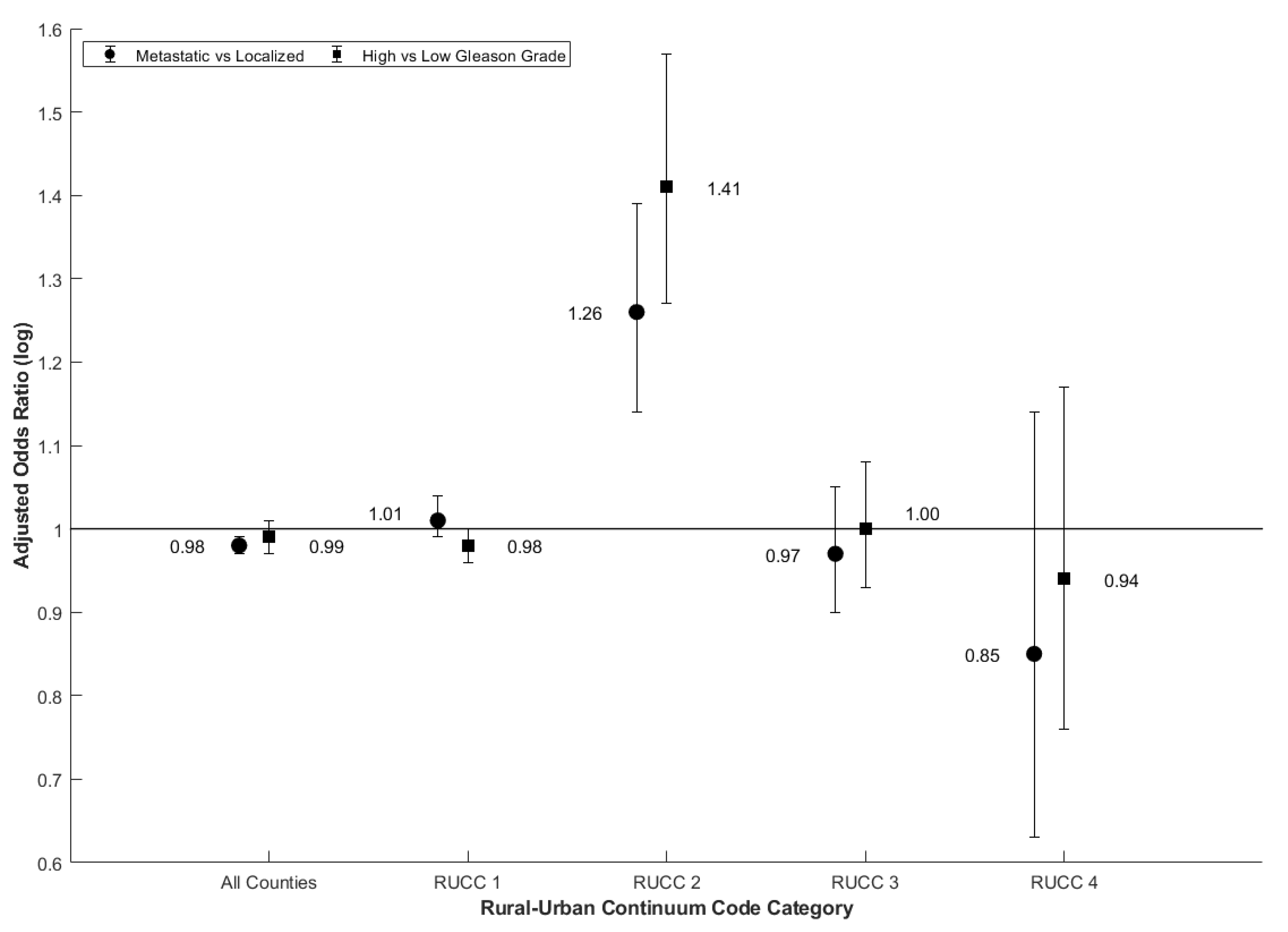
| Adjusted | 0.98 (0.98, 0.99) | 1.01 (0.99, 1.04) | 1.26 (1.14, 1.39) | 0.97 (0.90, 1.05) | 0.85 (0.63, 1.14) | 0.99 (0.97, 1.00) | 0.98 (0.96, 1.00) | 1.41 (1.27, 1.57) | 1.00 (0.93, 1.08) | 0.94 (0.76, 1.17) | |
| Arsenic OR (95% CI) | Unadjusted | 1.04 (1.02, 1.05) | 1.07 (1.05, 1.09) | 1.14 (1.09, 1.18) | 0.98 (0.92, 1.05) | 0.86 (0.64, 1.17) | 0.99 (0.97, 1.00) | 1.00 (0.99, 1.02) | 1.09 (1.02, 1.16) | 0.94 (0.88, 0.99) | 0.84 (0.68, 1.03) |
| Adjusted | 1.04 (1.02, 1.06) | 0.97 (0.95, 0.99) | 1.13 (1.08, 1.18) | 1.00 (0.92, 1.08) | 0.86 (0.49, 1.53) | 1.00 (0.98, 1.01) | 1.00 (0.97, 1.02) | 1.12 (1.06, 1.18) | 0.98 (0.91, 1.05) | 0.78 (0.50, 1.21) | |
| Lead OR (95% CI) | Unadjusted | 1.01 (0.99, 1.03) | 1.06 (1.02, 1.09) | 1.00 (0.96, 1.03) | 0.97 (0.91, 1.04) | 0.87 (0.73, 1.03) | 1.00 (0.99, 1.02) | 1.02 (0.99, 1.04) | 1.03 (1.00, 1.07) | 0.99 (0.94, 1.05) | 0.93 (0.83, 1.03) |
| Adjusted | 1.04 (1.03, 1.06) | 0.99 (0.94, 1.04) | 1.00 (0.96, 1.04) | 0.98 (0.91, 1.07) | 0.90 (0.76, 1.07) | 1.04 (1.02, 1.06) | 1.04 (1.00, 1.08) | 1.04 (1.01, 1.08) | 1.03 (0.97, 1.10) | 0.92 (0.80, 1.05) | |
| Measure of Aggressiveness | County Type | Race | Cadmium OR (95% CI) | Arsenic OR (95% CI) | Lead OR (95% CI) |
|---|---|---|---|---|---|
| Metastatic vs. Not | All | All | 0.98 (0.98, 0.99) | 1.04 (1.02, 1.06) | 1.04 (1.03, 1.06) |
| White | 1.01 (0.99, 1.03) | 1.03 (1.01, 1.06) | 1.01 (0.98, 1.03) | ||
| Black | 1.01 (0.97, 1.05) | 0.97 (0.93, 1.01) | 1.06 (1.00, 1.12) | ||
| RUCC 1 | All | 1.01 (0.99, 1.04) | 0.97 (0.95, 0.99) | 0.99 (0.94, 1.04) | |
| White | 1.06 (1.03, 1.08) | 0.94 (0.91, 0.97) | 1.03 (0.97, 1.09) | ||
| Black | 1.02 (0.96, 1.07) | 0.96 (0.92, 1.01) | 1.05 (0.98, 1.14) | ||
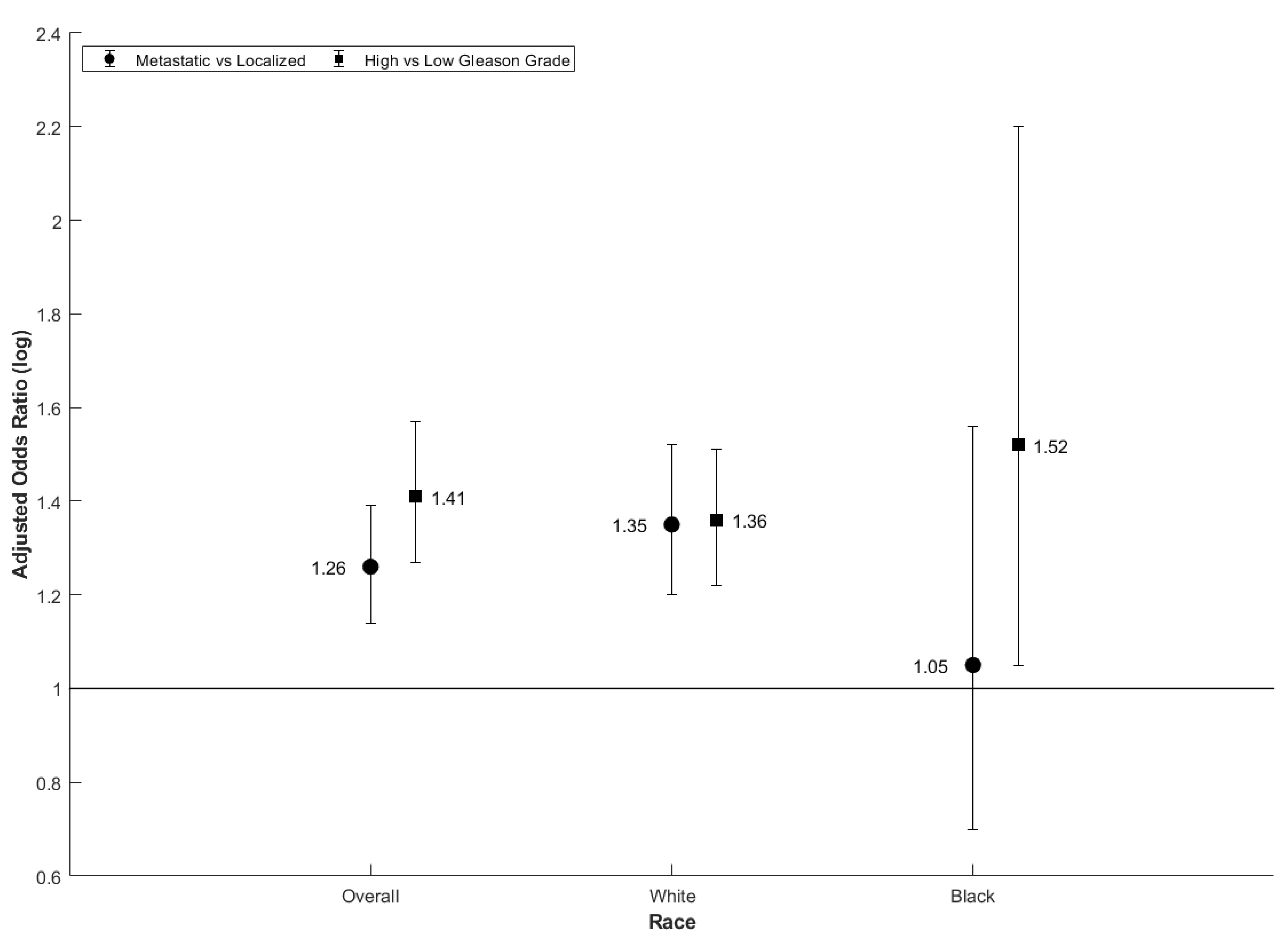
| RUCC 2 | All | 1.26 (1.14, 1.39) | 1.13 (1.08, 1.18) | 1.00 (0.96, 1.04) | |
| White | 1.35 (1.2, 1.52) | 1.17 (1.10, 1.23) | 1.00 (0.96, 1.05) | ||
| Black | 1.05 (0.7, 1.56) | 0.98 (0.75, 1.27) | 1.03 (0.80, 1.31) | ||
| RUCC 3 | All | 0.97 (0.90, 1.05) | 1.00 (0.92, 1.08) | 0.98 (0.91, 1.07) | |
| White | 1.00 (0.91, 1.10) | 1.04 (0.95, 1.15) | 0.95 (0.86, 1.04) | ||
| Black | 0.87 (0.70, 1.07) | 0.89 (0.75, 1.06) | 1.22 (0.99, 1.50) | ||
| RUCC 4 | All | 0.85 (0.63, 1.14) | 0.86 (0.49, 1.53) | 0.90 (0.76, 1.07) | |
| White | 0.89 (0.66, 1.21) | 0.88 (0.49, 1.60) | 0.90 (0.73, 1.11) | ||
| Black | 0.49 (0.04, 5.32) | 2.47 (0.09, 70.72) | 0.77 (0.34, 1.72) | ||
| High vs. Low Gleason Grade | All | All | 0.99 (0.97, 1.00) | 1.00 (0.98, 1.01) | 1.04 (1.02, 1.06) |
| White | 0.98 (0.97, 1.00) | 0.99 (0.97, 1.01) | 1.04 (1.02, 1.06) | ||
| Black | 0.97 (0.93, 1.02) | 0.95 (0.92, 0.99) | 1.02 (0.96, 1.09) | ||
| RUCC 1 | All | 0.98 (0.96, 1.00) | 1.00 (0.97, 1.02) | 1.04 (1.00, 1.08) | |
| White | 0.98 (0.95, 1.00) | 1.00 (0.97, 1.03) | 1.05 (1.01, 1.10) | ||
| Black | 0.97 (0.92, 1.03) | 0.95 (0.91, 0.99) | 0.96 (0.89, 1.04) | ||
| RUCC 2 | All | 1.41 (1.27, 1.57) | 1.12 (1.06, 1.18) | 1.04 (1.01, 1.08) | |
| White | 1.36 (1.22, 1.51) | 1.01 (0.96, 1.06) | 1.05 (1.01, 1.09) | ||
| Black | 1.52 (1.05, 2.20) | 1.24 (0.96, 1.60) | 1.17 (0.99, 1.39) | ||
| RUCC 3 | All | 1.00 (0.93, 1.08) | 0.98 (0.91, 1.05) | 1.03 (0.97, 1.10) | |
| White | 0.96 (0.88, 1.05) | 0.94 (0.86, 1.03) | 1.02 (0.95, 1.10) | ||
| Black | 1.28 (1.10, 1.50) | 1.06 (0.93, 1.20) | 1.12 (0.94, 1.34) | ||
| RUCC 4 | All | 0.94 (0.76, 1.17) | 0.78 (0.50, 1.21) | 0.92 (0.80, 1.05) | |
| White | 0.94 (0.76, 1.17) | 0.74 (0.47, 1.17) | 0.93 (0.80, 1.08) | ||
| Black | 1.26 (0.16, 9.83) | 1.30 (0.04, 37.91) | 0.82 (0.53, 1.27) |
| Measure of Aggressiveness | County Type | Age | Cadmium OR (95% CI) | Arsenic OR (95% CI) | Lead OR (95% CI) |
|---|---|---|---|---|---|
| Metastatic vs. Not | All | All | 0.98 (0.98, 0.99) | 1.04 (1.02, 1.06) | 1.04 (1.03, 1.06) |
| ≤60 | 1.05 (1.02, 1.08) | 1.03 (1.00, 1.06) | 1.07 (1.03, 1.10) | ||
| 61–70 | 1.02 (1.00, 1.05) | 1.01 (0.98, 1.03) | 1.04 (1.01, 1.07) | ||
| 71+ | 0.99 (0.97, 1.01) | 1.03 (1.00, 1.06) | 0.99 (0.96, 1.03) | ||
| RUCC 1 | All | 1.01 (0.99, 1.04) | 0.97 (0.95, 0.99) | 0.99 (0.94, 1.04) | |
| ≤60 | 1.07 (1.03, 1.12) | 1.03 (0.98, 1.07) | 1.14 (1.06, 1.23) | ||
| 61–70 | 1.03 (0.99, 1.08) | 0.97 (0.94, 1.01) | 1.09 (1.03, 1.15) | ||
| 71+ | 0.99 (0.96, 1.03) | 0.95 (0.92, 0.98) | 1.06 (1.01, 1.11) | ||
| RUCC 2 | All | 1.26 (1.14, 1.39) | 1.13 (1.08, 1.18) | 1.00 (0.96, 1.04) | |
| ≤60 | 1.25 (0.98, 1.59) | 1.16 (1.03, 1.30) | 1.06 (0.97, 1.14) | ||
| 61–70 | 1.33 (1.12, 1.57) | 1.16 (1.02, 1.26) | 0.99 (0.91, 1.06) | ||
| 71+ | 1.30 (1.02, 1.64) | 1.12 (1.01, 1.24) | 0.99 (0.92, 1.06) | ||
| RUCC 3 | All | 0.97 (0.90, 1.05) | 1.00 (0.92, 1.08) | 0.98 (0.91, 1.07) | |
| ≤60 | 0.84 (0.69, 1.01) | 0.93 (0.78, 1.11) | 1.09 (0.88, 1.36) | ||
| 61–70 | 1.01 (0.88, 1.16) | 1.03 (0.90, 1.18) | 0.97 (0.85, 1.11) | ||
| 71+ | 0.98 (0.87, 1.10) | 0.97 (0.85, 1.11) | 1.02 (0.85, 1.22) | ||
| RUCC 4 | All | 0.85 (0.63, 1.14) | 0.86 (0.49, 1.53) | 0.90 (0.76, 1.07) | |
| ≤60 | 1.03 (0.53, 2.08) | 0.99 (0.29, 3.34) | 0.94 (0.61, 1.45) | ||
| 61–70 | 0.87 (0.56, 1.37) | 0.31 (0.09, 1.05) | 0.89 (0.64, 1.25) | ||
| 71+ | 0.91 (0.68, 1.21) | 1.31 (0.76, 2.26) | 0.91 (0.73, 1.15) | ||
| High vs. Low Gleason Grade | All | All | 0.99 (0.97, 1.00) | 1.00 (0.98, 1.01) | 1.04 (1.02, 1.06) |
| ≤60 | 1.01 (0.98, 1.04) | 1.03 (0.99, 1.06) | 1.06 (1.02, 1.09) | ||
| 61–70 | 1.00 (0.98, 1.01) | 0.99 (0.96, 1.01) | 1.03 (1.00, 1.05) | ||
| 71+ | 0.97 (0.95, 0.99) | 1.00 (0.98, 1.03) | 1.04 (1.02, 1.07) | ||
| RUCC 1 | All | 0.98 (0.96, 1.00) | 1.00 (0.97, 1.02) | 1.04 (1.00, 1.08) | |
| ≤60 | 1.01 (0.97, 1.06) | 1.03 (0.98, 1.08) | 1.11 (1.02, 1.20) | ||
| 61–70 | 1.00 (0.97, 1.03) | 0.99 (0.95, 1.02) | 1.02 (0.96, 1.08) | ||
| 71+ | 0.96 (0.93, 0.99) | 1.01 (0.97, 1.05) | 1.05 (0.99, 1.12) | ||
| RUCC 2 | All | 1.41 (1.27, 1.57) | 1.12 (1.06, 1.18) | 1.04 (1.01, 1.08) | |
| ≤60 | 1.46 (1.19, 1.80) | 1.17 (1.05, 1.29) | 1.06 (0.99, 1.13) | ||
| 61–70 | 1.33 (1.17, 1.51) | 1.10 (1.04, 1.17) | 1.02 (0.97, 1.08) | ||
| 71+ | 1.49 (1.21, 1.84) | 1.12 (1.01, 1.23) | 1.06 (0.99, 1.12) | ||
| RUCC 3 | All | 1.00 (0.93, 1.08) | 0.98 (0.91, 1.05) | 1.03 (0.97, 1.10) | |
| ≤60 | 1.09 (0.96, 1.24) | 1.04 (0.92, 1.19) | 1.06 (0.91, 1.24) | ||
| 61–70 | 1.11 (1.01, 1.21) | 1.02 (0.92, 1.13) | 1.06 (0.97, 1.16) | ||
| 71+ | 0.96 (0.85, 1.07) | 0.91 (0.82, 1.02) | 0.99 (0.89, 1.11) | ||
| RUCC 4 | All | 0.94 (0.76, 1.17) | 0.78 (0.50, 1.21) | 0.92 (0.80, 1.05) | |
| ≤60 | 1.08 (0.70, 1.68) | 0.80 (0.36, 1.76) | 0.98 (0.72, 1.35) | ||
| 61–70 | 0.83 (0.59, 1.18) | 0.51 (0.24, 1.08) | 0.87 (0.71, 1.08) | ||
| 71+ | 1.01 (0.76, 1.34) | 1.06 (0.58, 1.93) | 1.01 (0.83, 1.22) |
Publisher’s Note: MDPI stays neutral with regard to jurisdictional claims in published maps and institutional affiliations. |
© 2021 by the authors. Licensee MDPI, Basel, Switzerland. This article is an open access article distributed under the terms and conditions of the Creative Commons Attribution (CC BY) license (https://creativecommons.org/licenses/by/4.0/).
Share and Cite
Vijayakumar, V.; Abern, M.R.; Jagai, J.S.; Kajdacsy-Balla, A. Observational Study of the Association between Air Cadmium Exposure and Prostate Cancer Aggressiveness at Diagnosis among a Nationwide Retrospective Cohort of 230,540 Patients in the United States. Int. J. Environ. Res. Public Health 2021, 18, 8333. https://doi.org/10.3390/ijerph18168333
Vijayakumar V, Abern MR, Jagai JS, Kajdacsy-Balla A. Observational Study of the Association between Air Cadmium Exposure and Prostate Cancer Aggressiveness at Diagnosis among a Nationwide Retrospective Cohort of 230,540 Patients in the United States. International Journal of Environmental Research and Public Health. 2021; 18(16):8333. https://doi.org/10.3390/ijerph18168333
Chicago/Turabian StyleVijayakumar, Vishwaarth, Michael R. Abern, Jyotsna S. Jagai, and André Kajdacsy-Balla. 2021. "Observational Study of the Association between Air Cadmium Exposure and Prostate Cancer Aggressiveness at Diagnosis among a Nationwide Retrospective Cohort of 230,540 Patients in the United States" International Journal of Environmental Research and Public Health 18, no. 16: 8333. https://doi.org/10.3390/ijerph18168333
APA StyleVijayakumar, V., Abern, M. R., Jagai, J. S., & Kajdacsy-Balla, A. (2021). Observational Study of the Association between Air Cadmium Exposure and Prostate Cancer Aggressiveness at Diagnosis among a Nationwide Retrospective Cohort of 230,540 Patients in the United States. International Journal of Environmental Research and Public Health, 18(16), 8333. https://doi.org/10.3390/ijerph18168333